Stability of FFLO states in optical lattices with bilayer structure

Abstract

We investigate the stability of the superfluid state in a bilayer fermionic optical lattice system with a confining potential, using the Bogoliubov de-Gennes equations. It is clarified that in the imbalanced case, the introduction of the interlayer hopping stabilizes the radial Fulde-Ferrell-Larkin-Ovchinnikov (FFLO) state, while makes the angular FFLO state unstable. We also discuss the system size dependence of the superfluid ground state. It is clarified that in a certain ring region the A-FFLO state is indeed realized in a large system.

1 Introduction

Recently ultracold atomic gases have attracted much interest since the successful realization of Bose-Einstein condensation (BEC) in a bosonic ⁸⁷Rb system.[1] Among them, an ultracold gas system in a periodic potential, so-called, an optical lattice system, [2, 3, 4, 5, 6] has been providing an ideal stage for experimental and theoretical studies of fundamental problems in condensed matter physics. Due to its high controllability in interaction strength, particle number, and other parameters, many remarkable phenomena have been observed such as a phase transition between a Mott insulator and a superfluid in bosonic systems,[7] and a crossover between the Bardeen-Cooper-Schrieffer (BCS) state and the BEC state in fermionic systems.[8, 9, 10] In addition, the superfluid state in the spin-imbalanced fermionic systems has been realized in a fermionic ⁶Li system,[11, 12] which stimulates further theoretical investigations on the superfluid state and its related phenomena.

An interesting question for the fermionic optical lattice system with imbalanced populations is how the symmetry-breaking state is realized at low temperatures. Various ground states have already been proposed to be more stable than the polarized superfluid (PSF) state.[13, 14] One of the probable candidates is the Fulde-Ferrell-Larkin-Ovchinnikov (FFLO) phase, [15, 16] where Cooper pairs are formed with a finite total momentum. This phase has been observed in the high field region in $\rm CeCoIn_{5}$ [17, 18, 19] and has theoretically been discussed in the compound[20, 21, 22, 23] as well as cold atoms with imbalanced populations. [24, 25, 26, 28, 29, 30, 27] In the two dimensional optical lattice with a confining potential, it has been pointed out that two kinds of the FFLO states are realized such as the radial-FFLO (R-FFLO)[31, 32] and the angular-FFLO (A-FFLO) states.[33, 34] In the former state, the superfluid order parameter changes its sign along the radial direction. In the latter, the order parameter oscillates along the angular direction, and the $C_{4v}$ symmetry as well as $U(1)$ symmetry are broken. On the other hand, such FFLO states with a three-dimensional structure have not been studied so well although the interlayer coupling should be important for realistic optical lattice systems.[35]

To make this point clear, we systematically study the two-dimensional optical lattice system with a bilayer structure as a simple model, which is schematically shown in Fig. 1.

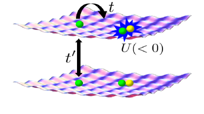
Figure 1: (Color online) Optical lattice with a bilayer structure

We discuss how the interlayer hopping between two layers affects ground state properties by means of the Bogoliubov de-Gennes (BdG) equation. We then clarify how the R-FFLO and A-FFLO states are realized in the optical lattice with a confining potential. The system size dependence of the ground state is also discussed.

The paper is organized as follows. In §2, we introduce the model Hamiltonian for the two-component fermions in the optical lattice and briefly summarize our theoretical approach. In §3, we discuss the stability of the R- and A-FFLO states in the bilayer optical lattice system. Scaling behavior in ground state properties is addressed in §4. A summary is given in the final section.

2 Model and Method

We study two-component ultracold fermions trapped in a two-dimensional bilayer optical lattice, which should be described by the following Hubbard Hamiltonian,

$$\begin{split}\hat{H}&=-t\sum_{\langle{ij}\rangle\sigma\alpha}\left(\hat{c}^{\dagger}_{i\alpha\sigma}\hat{c}_{j\alpha\sigma}+h.c.\right)\\ &-t^{\prime}\sum_{i\sigma}\left(\hat{c}^{\dagger}_{i1\sigma}\hat{c}_{i2\sigma}+h.c.\right)\\ &+\sum_{i\alpha\sigma}\left(V_{i}-\mu-h\sigma\right)\hat{n}_{i\alpha\sigma}+U\sum_{i\alpha}\hat{n}_{i\alpha\uparrow}\hat{n}_{i\alpha\downarrow}\end{split}$$ (1)

where $\langle{ij}\rangle$ indicates the nearest neighbors in each layer with $L\times L$ sites. $\hat{c}_{i\alpha\sigma}$ ($\hat{c}^{\dagger}_{i\alpha\sigma}$) annihilates (creates) a fermion at the $i$th site of $\alpha(=1,2)$th layer with spin $\sigma$ (=$\uparrow$ , $\downarrow$), and $\hat{n}_{i\alpha\sigma}={\hat{c}}_{i\alpha\sigma}^{\dagger}{\hat{c}}_{i\alpha\sigma}$. $t(t^{\prime})$ is the intralayer (interlayer) hopping and $U(<0)$ is the attractive interaction. The total number of particles $N(=N_{\uparrow}+N_{\downarrow})$ and the imbalanced population $P[=(N_{\uparrow}-N_{\downarrow})/(N_{\uparrow}+N_{\downarrow})]$, where $N_{\sigma}=\sum_{i\alpha}\langle\hat{c}_{i\alpha\sigma}^{\dagger}\hat{c}_{i\alpha\sigma}\rangle$, are tuned by the chemical potential $\mu$ and the magnetic field $h$ although these quantities can be controlled directly in the experiments. The confining potential is defined by $V_{i\alpha}=\beta(r_{i\alpha}/a)^{2}$, where $\beta(>0)$ is the curvature of the harmonic potential, $r_{i\alpha}$ is the distance measured from the center of the $\alpha$th layer, and $a$ is the lattice constant.

In the mean-field approach, the interaction term should be given as

$$\begin{split}U{\hat{n}}_{i\alpha\uparrow}{\hat{n}}_{i\alpha\downarrow}&\rightarrow U\sum_{\sigma}{\hat{n}}_{i\alpha\sigma}n_{i\alpha\bar{\sigma}}-Un_{i\alpha\uparrow}n_{i\alpha\downarrow}\\ &+\Delta_{i\alpha}^{*}{\hat{c}}_{i\alpha\downarrow}{\hat{c}}_{i\alpha\uparrow}+\Delta_{i\alpha}{\hat{c}}_{i\alpha\uparrow}^{\dagger}{\hat{c}}_{i\alpha\downarrow}^{\dagger}-\frac{1}{U}|\Delta_{i\alpha}|^{2},\end{split}$$ (2)

where $\Delta_{i\alpha}=U\langle\hat{c}_{i\downarrow\alpha}\hat{c}_{i\uparrow\alpha}\rangle$ is the local superfluid order parameter, and $n_{i\sigma\alpha}=\langle\hat{c}^{\dagger}_{i\sigma\alpha}\hat{c}_{i\sigma\alpha}\rangle$ is the local particle density. The BdG equations should be written in terms of the $4L^{2}\times 4L^{2}$ matrix, as

$$\sum_{j}\left(\begin{array}[]{ccc}{\bf H}^{(1)}_{ij}&{\bf T}_{ij}\\ {\bf T}_{ij}&{\bf H}^{(2)}_{ij}\\ \end{array}\right)\left(\begin{array}[]{ccc}{\bf{\phi}}^{(1)}_{qj}\\ {\bf{\phi}}^{(2)}_{qj}\\ \end{array}\right)=\epsilon_{q}\left(\begin{array}[]{ccc}{\bf{\phi}}^{(1)}_{qi}\\ {\bf{\phi}}^{(2)}_{qi}\\ \end{array}\right)$$ (3)

$${\bf H}^{(\alpha)}_{ij}=\left(\begin{array}[]{ccc}H^{\alpha}_{ij\uparrow}&\Delta_{ij}^{\ast}\\ {\Delta}_{ij}&-H^{\alpha}_{ij\downarrow}\\ \end{array}\right)$$ (4)

$${\bf T}_{ij}=\left(\begin{array}[]{ccc}K_{ij}&0\\ 0&-K_{ij}\\ \end{array}\right)$$ (5)

where $H^{\alpha}_{ij\sigma}=-t\delta_{\langle ij\rangle}+(-\mu-h\sigma+Un_{i\alpha\bar{\sigma}})\delta_{ij}$, $K_{ij}=-t^{\prime}\delta_{ij}$, and $\Delta_{ij}={\Delta}_{i}\delta_{ij}$, where $\delta_{ij}$ is the Kronecker delta. The eigenfunctions $\phi^{(\alpha)}_{qi}={}^{t}(u^{(\alpha)}_{qi\uparrow},v^{(\alpha)}_{qi\downarrow})$ indicate the Bogoliubov quasiparticle amplitudes at the $i$th site on the $\alpha$th layer. The mean fields are then determined by the self-consistent equations as

$$\Delta_{i\alpha} = U\sum_{q}u^{(\alpha)}_{qi}v^{(\alpha)}_{qi}f(\epsilon_{q}),$$ (6)

$$n_{i\alpha\uparrow} = \sum_{q}\left|u^{(\alpha)}_{qi}\right|^{2}f(\epsilon_{q}),$$ (7)

$$n_{i\alpha\downarrow} = \sum_{q}\left|v^{(\alpha)}_{qi}\right|^{2}f(-\epsilon_{q})$$ (8)

where $f(\epsilon)$ = $[\exp(\epsilon/T)+1]^{-1}$ is the Fermi distribution function and $T$ is the temperature.

In the iterative method, one sometimes reaches the metastable state with the higher energy than the ground state. Therefore, it is important to choose an appropriate initial state in this treatment. In this paper, to discuss the stability of the FFLO states, we use the symmetry breaking states with $n$-fold symmetry in space and solve the BdG equations iteratively. Then we determine the ground state by comparing the free energies of their converged solutions.

For convenience, we define the characteristic length of the potential as $d=\sqrt{t/\beta}a$ and the effective particle density as $\tilde{\rho}=Na^{2}/\pi d^{2}$. We set $t$ as a unit of energy and fix the interaction strength and the temperature as $U/t=-4$ and $T/t=0.001$, for simplicity. The temperature is low enough, which enables us to discuss ground state properties in the bilayer optical lattice system. The obtained ground state always has a mirror symmetry in the case $t^{\prime}/t\neq 0$. Therefore, in this paper, we will show the results for one of the layers to discuss the stability of the superfluid state.

3 Stability of the superfluid state

In the section, we focus on the optical lattice system ($L=30$) with the confining potential $\beta=0.04$ $(d=5a)$ to discuss how the introduction of the interlayer hopping affects the stability of the BCS, R-FFLO and A-FFLO states. Before starting discussions, we would like to mention the characteristic profiles for these states. When the magnetic field is small enough, the BCS state is realized, where the finite pair potential appears without the magnetization. In the R-FFLO or A-FFLO states, the magnetization is finite, and the sign changes appear in the pair potential, depending on the direction of its oscillation. Namely, the sign change in the radial direction appears in the former state. On the other hand, it appears in a certain ring region in the latter state. Note that the BCS and R-FFLO states have the same spatial symmetry, in contrast to the A-FFLO state. Therefore, the BCS state is adiabatically connected to the R-FFLO state through the crossover.

We first study ground state properties of the dilute system with $\tilde{\rho}\simeq 0.89$ $(N\simeq 70)$. In the case with $t^{\prime}/t=h/t=0$, the particles are smoothly distributed and the order parameter appears around the center of the system. The local particle density $N_{i}=\sum_{\sigma}n_{i\alpha\sigma}$ and local order parameter $\Delta_{i}$ for each layer are shown in Fig. 2.

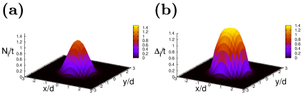
Figure 2: Profiles of the particle density $N_{i}$ and the order parameter $\Delta_{i}$ in the dilute system with $\tilde{\rho}\simeq 0.89$, $t^{\prime}/t=0.0$ and $P=0$.

When the magnetic field is applied, three kinds of ground states appear. In the case $h<h^{\prime}(\sim 0.7t)$, the BCS state is realized. In the intermediate region $h^{\prime}<h<h_{c}(\sim 1.4t)$, the R-FFLO state is realized, where the magnetization appears in the system and the order parameter changes its sign along the radial direction. Beyond the critical field $h_{c}$, the pair potential is no longer finite, and the ground state is paramagnetic. Here we focus on the system with $h/t=0.6$ to discuss the effect of the interlayer hopping. The cross-sections of the order parameter and the magnetization, which is defined by $m_{i}=n_{i\alpha\uparrow}-n_{i\alpha\downarrow}$, are shown in Fig. 3.

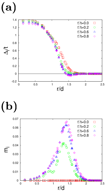
Figure 3: (Color online) Profile of the order parameter $\Delta_{i}$ (a) and the magnetization $m_{i}$ (b) as a function of $r/d$ in the dilute system.

When the interlayer hopping $t^{\prime}$ is small, the system belongs to the BCS state, where the order parameter appears around the center of the potential ($r/d<1.7$). The introduction of the interlayer hopping reduces the pair potential, typically around $r/d\sim 1.5$. At last, the sign change appears in the superfluid order parameter although it may not be visible in the case $t^{\prime}/t=0.2$ in Fig. 3 (a). In addition, the magnetization is induced in the vicinity of the sign change point, as shown in Fig. 3 (b). This suggests the realization of the R-FFLO state. Further increase in the interlayer hopping yields a clear sign change in the order parameter and increases the magnetization monotonically. Therefore, we can say that the interlayer hopping stabilizes the R-FFLO state.

By performing similar calculations, we obtain the phase diagram of the dilute system, as shown in Fig. 4.

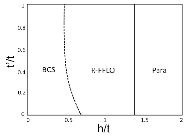
Figure 4: Phase diagram of the dilute system with $\tilde{\rho}\simeq 0.89$

.

The crossover between the BCS state and the R-FFLO state is roughly estimated by the appearance of the magnetization, which is shown as a dashed line. The interlayer hopping $t^{\prime}$ little affects the phase boundary between the R-FFLO and normal states, in contrast to the crossover boundary.

Next, we study ground state properties of the dense system with $\tilde{\rho}\simeq 6.4$ ($N\simeq 500$). In the case, a doubly occupied (Fock) state is realized around the center of the system due to the attractive interaction and the trap potential, as shown in Fig. 5 (a). Therefore, when $h/t=0.0$, the superfluid state is realized away from the center and the doughnutlike structure appears in the pair potential, as shown in Fig. 5 (b).

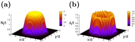
Figure 5: Profiles of the particle density $N_{i}$ and the order parameter $\Delta_{i}$ in the dense system with $\tilde{\rho}\simeq 6.4$, $t^{\prime}/t=0.0$ and $P=0$.

When the spin imbalanced population is introduced, the R-FFLO and A-FFLO states are realized in the cases $(h^{\prime}<h<h_{c1})$ and $(h_{c1}<h<h_{c2})$, where $h^{\prime}=0.6t$, $h_{c1}=1.1t$ and $h_{c2}=1.4t$. We here focus on the latter case with $h/t=1.3$, where oscillation behavior with nine peaks in the order parameter appear in a certain ring region, as shown in Fig. 6 (a). The introduction of the interlayer hopping $t^{\prime}$ monotonically decreases the magnitude of the order parameters, as shown in Fig. 6.

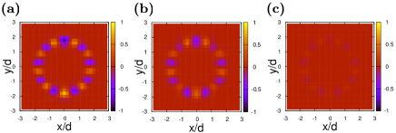
Figure 6: (Color online) Order parameter $\Delta_{i}$ in the dense system when $t^{\prime}/t=0.0,0.6$ and $1.0$ (from the left to the right).

Finally it vanishes and the phase transition occurs to the paramagnetic state. This instability should be explained by the following. In the A-FFLO state, the oscillation of the order parameter appears in a certain ring region, which implies that one dimensional structure plays an important role to be stabilized. In this point of view, the interlayer coupling can be regarded as the introduction of the two-dimensional structure. Therefore, the A-FFLO state becomes unstable against the interlayer coupling.

To discuss how the magnetic field affects the nature of the superfluid state, we also show the number of peaks in the angular direction $M$ and the average of the order parameter, which is defined by $\bar{\Delta}=\sum_{i}|\Delta_{i}|/N_{\downarrow}$, in Fig. 7.

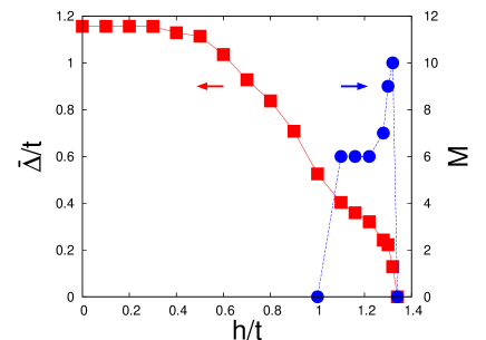
Figure 7: (Color online) Squares and circles represent the average and the number of peaks in the angular direction of the order parameter in the dense system with $t^{\prime}/t=0.6$.

When $h/t=0.0$, the BCS state is realized with $\bar{\Delta}/t\sim 1.2$ and $M=0$. Applying the magnetic field, $\bar{\Delta}$ is little changed up to $h=h^{\prime}(\sim 0.3t)$ and begins to decrease beyond it. This means that the crossover occurs to the R-FFLO state at $h=h^{\prime}$, where the sign change in the order parameter reduces $\bar{\Delta}$. Further increase in the magnetic field monotonically decreases the quantity. When $h=h_{c1}$, oscillation behavior suddenly appears in the angular direction of the order parameter $(M=6)$, and the phase transition occurs to the A-FFLO state. The R-FFLO and A-FFLO states have different spatial structures in the magnetization and order parameter. For example, the sign change in the order parameter appears in the radial and angular direction, which means that these states are not adiabatically connected to each other around $h=h_{c1}$. This is contrast to the results for one-dimensional system, where the second-order phase transition occurs between the BCS and FFLO states.[36] When the system approaches the phase boundary ($h_{c2}\sim 1.4t$), $\bar{\Delta}$ is rapidly decreased and $M$ is increased. This may originate from the fact that the magnetization can be induced around the regions with $\Delta_{i\alpha}/t\sim 0$. Therefore, when the large magnetic field is applied, many peaks appear in the profile of the order parameters. This tendency is essentially the same as the single layer optical lattice.[33] Finally, the order parameter vanishes at $h=h_{c2}$, where the phase transition occurs to the normal state.

By performing the similar calculations, we obtain the phase diagram shown in Fig. 8.

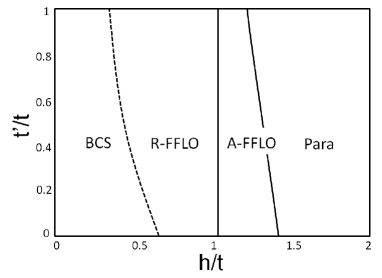
Figure 8: Phase diagram for the dense system with $\tilde{\rho}\simeq 6.4$

.

It is found that the interlayer hopping stabilizes the R-FFLO state, which is the same as the dilute case. On the other hand, the A-FFLO state becomes unstable against the interlayer hopping.

We have treated the bilayer system to discuss how the interlayer hopping affects the stability of the FFLO states. Although the treated model is simple to discuss ground state properties of the layered optical lattice system, we believe that the obtained results capture the essence of the interlayer hopping. Namely, the A-FFLO state with interesting spatial properties survives in the system with a small interlayer hopping. In the following section, we discuss how the FFLO states are realized in the large system.

4 Size dependence of FFLO states

In the section, we study the stability of the FFLO states in the larger system. It is naively expected that low energy properties in the system are scaled by the characteristic length of the harmonic potential. By contrast, the characteristic length of the FFLO state should depend on the spin imbalance in the system, which is not directly related to the length $d$, as discussed in the previous section. Therefore, it is necessary to clarify how interesting low energy properties are changed by the system size.

To discuss scaling behavior in the system carefully, we fix the confining potential at four edges of the system as $V_{i\alpha}=18t$, and keep the effective particle density and the spin imbalance as $\tilde{\rho}=6.4$ and $P=0.15$. The cross-sections of the particle density and the order parameter are obtained, as shown in Fig. 9. In the BCS case (not shown), the profiles are well scaled, and thereby the state is stable in the large system. We find in Fig. 9 (a) that in the R-FFLO state, a main peak structure in the order parameter is scaled. However, a size dependence appears around the regions with a sign change ($r/d\sim 1.3$ and 2.2). Since the dip structures tend to shrink on the increase of the system size, it may be difficult to observe them in a large system, as a signature for the realization of the R-FFLO state. As for the A-FFLO state, disorder behavior in the profiles of the order parameter and magnetization appears in the region $(1.5<r/d<2.0)$, which is reflected by the oscillation of these quantities in the angular direction, as shown in Fig. 9 (b). Nevertheless, their envelopes are well scaled, where the magnitude has a maximum at $r_{0}/d=1.75$. The spatial dependence of the order parameter and magnetization is also shown in Fig. 10. It is clearly found that each peak in the magnetization $m_{i}$ is located at the sign change point along a certain ring in the order parameter $\Delta_{i}$. These are consistent with the fact that the A-FFLO state is realized in the ring region. Increasing the system size, we find that the number of peaks in a certain ring region is increased. This means that the peak structure in the angular direction is not scaled.

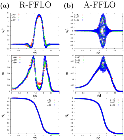
Figure 9: (Color online) Profiles of the order parameter $\Delta_{i}$, magnetization $m_{i}$, and particle density $N_{i}$ for the R-FFLO (a) and A-FFLO (b) states.

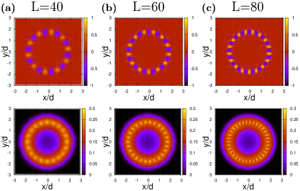
Figure 10: Order parameter (upper panel) and magnetization (lower panel) in the system with $t^{\prime}/t=0.6$, $\tilde{\rho}\simeq 6.4$, $P\simeq 0.15$, $L=40,60$, and $80$ (from the left to the right).

To clarify the size dependence of the oscillations, we also calculate the wave number defined by $k_{\rm{A-FFLO}}=M/r_{0}$, where $M$ is the number of the peaks in the order parameter. Fig. 11 shows that it approaches a certain value $k_{\rm{A-FFLO}}\sim 0.7/a$ when the system size is increased. These imply that there indeed exists a region with the A-FFLO state, and it is connected to the FFLO state expected in the one-dimensional Fermi gases. The characteristic wave number does not depend on the system size, but on the imbalanced populations. Therefore, we can say that the A-FFLO state should be realized in the thermodynamic limit $(L\rightarrow\infty)$ if the interlayer hopping is small enough.

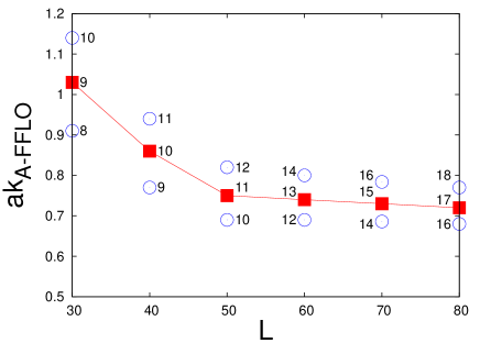
Figure 11: Squares (circles) represent the wave number characteristic of the A-FFLO state for the ground (meta-stable) state. The number indicates peaks in the pair potential.

Before closing this section, we wish to comment on the possibility of the supersolid state. In the attractive Hubbard model on the bipartite lattice in two or higher dimensions, it is known that the density wave ground state and the superfluid state are degenerate at half filling.[37, 38, 39] Therefore, in a certain narrow region with $\langle n_{i}\rangle\sim 1$, the supersolid state, where both the density wave state and superfluid state coexist, may be realized.[40] It is necessary to carefully deal with particle correlations beyond the BdG mean-field approach, which is now under considerations.

5 Summary

We have studied the stability of the superfluid state in a bilayer fermionic optical lattice system with imbalanced populations by means of the BdG equations. It has been clarified that the introduction of the hopping between two layers stabilizes the radial FFLO state, while makes the angular FFLO state unstable. We have also discussed scaling behavior in the superfluid state. It has been found that the wave number characteristic of the A-FFLO state approaches a certain value when the system size is increased. This implies that the A-FFLO state should be realized in the thermodynamic limit.

References

- [1] M. H. Anderson, J. R. Ensher, M. R. Matthews, C. E. Wieman, and E. A. Cornell, Science 269, 198 (1995).
- [2] I. Bloch and M. Greiner: Advances in Atomic, Molecular, and Optical Physics, edited by P. Berman and C. Lin (Academic Press, New York, 2005), Vol. 52 p. 1.
- [3] I. Bloch: Nature Physics 1 (2005) 23.
- [4] D. Jaksch and P. Zoller: Ann. Phys. (NY) 315 (2005) 52.
- [5] O. Morsch and M. Oberhaler: Rev. Mod. Phys. 78 (2006) 179.
- [6] J. K. Chin, D. E. Miller, Y. Liu, C. Stan, W. Setiawan, C. Sanner, K. Xu, and W. Ketterle: Nature 443 (2006) 05224.
- [7] M. Greiner, O. Mandel, T. Esslinger, T. W. Hänsch and I. Bloch: Nature 415 (2003) 39.
- [8] S. Jochim,M. Bartenstein, A. Altmeyer, G. Hendl, S. Riedl, C. Chin, J. Hecker Denschlag, and R. Grimm: Science 302, 2101 (2003).
- [9] M. W. Zwierlein,C. A. Stan, C. H. Schunck, S. M. F. Raupach, S. Gupta, Z. Hadzibabic, and W. Ketterle: Phys. Rev. Lett. 91, 250401 (2003).
- [10] T. Bourdel,L. Khaykovich, J. Cubizolles, J. Zhang, F. Chevy, M. Teichmann, L. Tarruell, S. J. J. M. F. Kokkelmans, and C. Salomon: Phys. Rev. Lett. 93, 050401 (2004).
- [11] M. W. Zwierlein, A. Schirotzek, C. H. Shunck, and W. Ketterle: Science 311 (2006) 492.
- [12] G. B. Partridge, W. Li, R. I. Kamar, Y. Liao, and R. G. Hulet: Science 311 (2006) 503.
- [13] T.-L. Dao, M. Ferrero, A. Georges, M. Capone, and O. Parcollet: Phys. Rev. Lett. 101 (2008) 236405.
- [14] A. Koga and P. Werner: J. Phys. Soc. Jpn. 79 (2010) 064401.
- [15] P. Fulde, R. A. Ferrell: Phys. Rev. 135 (1964) A550.
- [16] A. I. Larkin, Y. N. Ovhinnikov: Sov. Phys. JETP 20 (1965) 762.
- [17] H. A. Radovan, N. A. Fortune, T. P. Murphy, S. T. Hannahs, E. C. Palm, S. W. Tozer, and D. Hall: Nature 425 (2003) 51.
- [18] A. Bianchi, R. Movshovich, C. Capan, P. G. Pagliuso, and J. L. Sarrao: Phys. Rev. Lett. 91 (2003) 187004.
- [19] Y. Matsuda and H. Shimahara: J. Phys. Soc. Jpn. 76 (2007) 051005.
- [20] H. Adachi and R. Ikeda: Phys. Rev. B 68 (2003) 184510.
- [21] R. Ikeda: Phys. Rev. B 76 (2007) 054517.
- [22] Y. Yanase and M. Sigrist: J. Phys.: Conf. Ser. 150 (2009) 052287.
- [23] K. Miyake: J. Phys. Soc. Jpn. 77 (2008) 123703.
- [24] T. Mizushima, K. Machida, and M. Ichioka: Phys. Rev. Lett. 94 (2005) 060404.
- [25] P. Castorina, M. Grasso, M. Oertel, M. Urban, and D. Zappalá: Phys. Rev. A 72 (2005) 025601.
- [26] J. Kinnunen, L. M. Jensen, and P. Törmä: Phys. Rev. Lett. 96 (2006) 110403.
- [27] Xia-Ji Liu, Hui Hu, and Peter D. Drummond: Phys. Rev. A 76 (2007) 043605.
- [28] M. Tezuka and M. Ueda: Phys. Rev. Lett. 100, 110403 (2008).
- [29] J. P. A. Devreese, S. L. Klimin and J. Tempere: Phys. Rev. A 83, 013606 (2011).
- [30] M. Okumura, S. Yamada, M. Machida, and H. Aoki: Phys. Rev. A 83, 031606(R) (2011).
- [31] T. Mizushima, M. Ichioka, and K. Machida, J. Phys. Soc. Jpn. 76 (2007) 104006.
- [32] M. Iskin, C. J. Williams: Phys. Rev. A 78 (2008) 011603(R).
- [33] Y. Chen, Z. D. Wang, F. C. Zhang, and C. S. Ting: Phys. Rev. B 79 (2009) 054512.
- [34] Y. Yanase, Phys. Rev. B 80 (2009) 220510(R).
- [35] K. Martiyanov, V. Makhalov, and A. Turlapov: Phys. Rev. Lett. 105 (2010) 030404.
- [36] K. Machida and H. Nakanishi: Phys. Rev. B 30 (1984) 122.
- [37] H. Shiba: Prog. Theor. Phys. 48 (1972) 2171.
- [38] R. T. Scalettar, E. Y. Loh, J. E. Gubernatis, A. Moreo, S. R. White, D. J. Scalapino, R. L. Sugar, and E. Dagotto: Phys. Rev. Lett. 62 (1989) 1407.
- [39] J. K. Freericks, M. Jarrell, and D. J. Scalapino: Phys. Rev. B 48 (1993) 6302.
- [40] A. Koga, T. Higashiyama, K. Inaba, S. Suga and N. Kawakami: J. Phys. Soc. Jpn. 77 (2008) 073602; Phys. Rev. A 79 (2009) 013607.