Geometric measure of entanglement of multipartite mixed states

Abstract

The geometric measure of entanglement of a pure state, defined by its distance to the set of pure separable states, is extended to multipartite mixed states. We characterize the nearest disentangled mixed state to a given mixed state with respect to this measure by a system of equations. The entanglement eigenvalue for a mixed state is introduced. For a given mixed state, we show that its nearest disentangled mixed state is associated with its entanglement eigenvalue.

Key words:   quantum entanglement, geometric measure

1 Introduction

The quantum entanglement problem is regarded as a central problem in quantum information [9, 15, 10], and the geometric measure is one of the most important measures of quantum entanglement [1, 14, 16, 10]. It was first proposed by Shimony [14] and generalized to multipartite systems by Wei and Goldbart [16], and has become one of the widely used entanglement measures for multiparticle cases [7, 4, 2, 5, 11, 3, 6].

The geometric measure is based on the geometric distance between a given pure state and the set of separable pure states. From the definition, the quantum eigenvalue problem is derived to characterize the nearest separable pure state with respect to this measure [16, 5, 11]. This characterization is significant: the eigenvalues are always real numbers and the largest one corresponds to the maximal overlap of the given pure state and the separable pure states.

Based on the convex roof construction, this geometric measure is extended to multipartite mixed states [16]. Although the extension is standard, analogue characterizations for disentangled mixed states are not clear [16, 7]. Instead of the convex roof extension, we propose in this paper a natural extension of the geometric measure from pure states to mixed states. Most interestingly, a characterization for the nearest disentangled mixed state still holds. We show that there is a system of equations associated to the proposed geometric measure for mixed states. The entanglement eigenvalue for a mixed state is introduced and it is proven to be an indicator of the proposed geometric measure. Moreover, the disentangled mixed state corresponding to the entanglement eigenvalue is shown to be the nearest disentangled mixed state to the given mixed state with respect to this measure.

The rest of this paper is organized as follows. Some preliminaries are presented in Section 2 to include some basic definitions. The geometric measure of mixed states is proposed in Section 3. In Section 4, the characterization for the nearest disentangled mixed state is investigated. Section 5 concludes this paper with some remarks.

2 Preliminaries

An $m$-partite pure state $|\Psi\rangle$ of a composite quantum system can be regarded as a normalized element in a Hilbert tensor product space ${\mathcal{H}}=\bigotimes_{k=1}^{m}{\mathcal{H}}_{k}$, where the dimension of ${\mathcal{H}}_{k}$ is $d_{k}$ for $k=1,\ldots,m$. A separable $m$-partite pure state $|\Phi\rangle\in{\mathcal{H}}$ can be described by $|\Phi\rangle=\bigotimes_{k=1}^{m}|\phi^{(k)}\rangle$ with $|\phi^{(k)}\rangle\in{\mathcal{H}}_{k}$ and $\||\phi^{(k)}\rangle\|=1$ for $k=1,\ldots,m$. Denote by $Separ(\mathcal{H})$ the set of all separable pure states in $\mathcal{H}$. A state is called entangled if it is not separable.

For a given $m$-partite pure state $|\Psi\rangle\in{\mathcal{H}}$, a geometric measure is then defined as [16]

$$\min_{|\Phi\rangle\in Separ(\mathcal{H})}\||\Psi\rangle-|\Phi\rangle\|,$$ (1)

or one may consider

$$\min_{|\Phi\rangle\in Separ(\mathcal{H})}\frac{1}{2}\||\Psi\rangle-|\Phi\rangle\|^{2}=1-G(\Psi),$$ (2)

where $G(\Psi)$ is the maximal overlap:

$$G(\Psi)=\max_{|\Phi\rangle\in Separ(\mathcal{H})}|\langle\Psi|\Phi\rangle|.$$ (3)

Based on (2), the quantum eigenvalue problem is proposed and analyzed in [16, 11]:

$$\left\{\begin{array}[]{rcl}\langle\Psi|\left(\bigotimes_{j\neq k}|\phi^{(j)}\rangle\right)&=&\lambda\langle\phi^{(k)}|,\\ \left(\bigotimes_{j\neq k}\langle\phi^{(j)}|\right)\Psi\rangle&=&\lambda|\phi^{(k)}\rangle,\\ \||\phi^{(k)}\rangle\|&=&1,k=1,\ldots,m.\end{array}\right.$$ (7)

Proposition 2.1

Let $|\Psi\rangle\in{\cal H}$ be a pure state and the corresponding quantum eigenvalue problem be (7). Then, $\lambda$ is a real number and the maximal overlap in (3) is equal to the largest such $\lambda$.

Proof. See [16, Section II] or [11, Section 2] for the detailed proof. $\Box$

The largest $\lambda$ in (7), denoted by $\Lambda_{\max}$, is called the entanglement eigenvalue [16, 11]. Consequently, the geometric measure in (2) equals $1-\Lambda_{\max}$.

The entanglement problem for mixed states in ${\cal H}$ has attracted much attention as well [16, 7, 10, 3, 17, 13]. Usually, a mixed state in ${\cal H}$ is represented by a density matrix $\varrho$ of size $\prod_{k=1}^{m}d_{k}\times\prod_{k=1}^{m}d_{k}$ [7, 16, 18]. It is Hermitian, positive semidefinite and trace one. There are several concepts on disentangled multipartite mixed states. We adopt the following one [10].

Definition 2.1

For a mixed state in ${\cal H}$ with density matrix $\varrho$, it is disentangled if

$$\varrho=\sum_{k}p_{k}|\Psi^{(k)}\rangle\langle\Psi^{(k)}|$$

for some pure separable states $|\Psi^{(k)}\rangle\in Separ({\cal H})$, $p_{k}\geq 0$ and $\sum_{k}p_{k}=1$.

Denote by $Disen({\cal H})$ the set of all disentangled mixed states in ${\cal H}$.

The geometric measure for pure states can be extended to mixed states through the convex roof construction [16]:

$$E_{C}(\varrho):=\min_{\{p_{i},\Psi^{(i)}\}}\sum_{i}p_{i}M(|\Psi^{(i)}\rangle)$$ (8)

where the minimum is taken over all decompositions $\varrho=\sum_{i}p_{i}|\Psi^{(i)}\rangle\langle\Psi^{(i)}|$ into pure states with the $p_{i}$ forming a probability distribution, and the measure $M$ for pure states can be chosen to be both the measure (2) and any other measures.

3 Geometric measure for mixed states

Although the geometric measure defined in (8) satisfies the criteria for entanglement monotone [15, 16], the extension of Proposition 2.1 to mixed states is not clear and there lack characterizations of the nearest disentanglement mixed state to an arbitrary mixed state. In this section, instead of (8), we propose a geometric measure for mixed states which is a natural extension of (2).

Definition 3.1

For a mixed state in ${\cal H}$ with density matrix $\varrho$, its geometric measure is defined as:

$$E(\varrho):=\min_{\rho\in Disen({\cal H}),\;\|\rho\|=\|\varrho\|}\|\varrho-\rho\|,$$ (9)

where the norm is the Frobenius norm of matrices.

To see that Definition 3.1 is well-defined, the following lemma is essential.

Lemma 3.1

Let $\varrho$ be the density matrix of a mixed state in ${\cal H}$. Then the set $S(\varrho):=\{\rho\in Disen({\cal H})\;|\;\|\rho\|=\|\varrho\|\}$ is a nonempty compact set.

Proof. Let $n:=\Pi_{k=1}^{m}d_{k}$ and $N:=n^{2}+1$. The density matrix is an $n\times n$ Hermitian matrix. For any density matrix $\varrho$, its real part is a symmetric $n\times n$ matrix and its imaginary part is an skew-symmetric $n\times n$ matrix. Consequently, the real dimension of $Disen({\cal H})$ is $n^{2}$. By the definition of $Disen({\cal H})$, every $\rho\in Disen({\cal H})$ can be represented as a convex combination of density matrices of pure separable states. By Caratheodory’s theorem[12], the number of density matrices of pure separable states in such a combination can be chosen to be at most $N$. Consequently, we have

$$S(\varrho)=\left\{\begin{array}[]{cc}\begin{array}[]{c}\rho=\sum_{k=1}^{N}p_{k}|\phi_{1}^{(k)}\rangle\cdots|\phi^{(k)}_{m}\rangle\\ \langle\phi^{(k)}_{m}|\cdots\langle\phi^{(k)}_{1}|\end{array}&\left|\begin{array}[]{c}\left\||\phi^{(k)}_{i}\rangle\right\|^{2}=1,\;i=1,\ldots,m,\;k=1,\ldots,N,\\ \sum_{r,s=1}^{N}p_{r}p_{s}\prod_{i=1}^{m}\langle\phi^{(r)}_{i}|\phi^{(s)}_{i}\rangle\langle\phi^{(s)}_{i}|\phi^{(r)}_{i}\rangle=\|\varrho\|^{2},\\ \sum_{k=1}^{N}p_{k}=1,\;p_{k}\geq 0,\;k=1,\ldots,N.\end{array}\right.\end{array}\right\},$$

which is obviously bounded and closed. Since $\varrho$ a positive semidefinite $n\times n$ matrix, we can assume that $\varrho=\sum_{k=1}^{K}\alpha_{k}|\Psi^{(k)}\rangle\langle\Psi^{(k)}|$ be the orthogonal eigenvalue decomposition. Then, $\sum_{k=1}^{K}\alpha_{k}^{2}=\|\varrho\|^{2}$, and $\sum_{k=1}^{K}\alpha_{k}=1$ as $\mbox{Tr}(\varrho)=1$. Since $K\leq n$, we can find $\{|\phi^{(k)}_{1}\rangle,\ldots,|\phi^{(k)}_{m}\rangle\}_{k=1}^{K}$ such that

$$\begin{array}[]{c}\left\||\phi^{(k)}_{i}\rangle\right\|^{2}=1,\;i=1,\ldots,m,\;k=1,\ldots,K,\\ \prod_{i=1}^{m}\langle\phi^{(r)}_{i}|\phi^{(s)}_{i}\rangle=0,\;\forall r\neq s,\;r,s=1,\ldots,K.\end{array}$$

Consequently, $\rho:=\sum_{k=1}^{K}\alpha_{k}|\phi_{1}^{(k)}\rangle\cdots|\phi^{(k)}_{m}\rangle\langle\phi^{(k)}_{m}|\cdots\langle\phi^{(k)}_{1}|\in S(\varrho)$. The result follows. $\Box$

The following proposition concerns some properties of the measure (9).

Proposition 3.1

Let $\varrho$ be the density matrix of a mixed state in ${\cal H}$ and $E(\varrho)$ be defined as (9). Then, we have

• $E(\varrho)\geq 0$ and $E(\varrho)=0$ if and only if $\varrho\in Disen({\cal H})$.

• Local unitary transformations on $Disen({\cal H})$ do not change $E$.

Proof. (a) By (9), $E(\varrho)\geq 0$ for any $\varrho\in Disen({\cal H})$. If $\varrho\in Disen({\cal H})$, then with $\rho:=\varrho$, we get $\|\varrho-\rho\|=0$. consequently, $0\leq E(\varrho)\leq 0$ as desired. Now, suppose that $E(\varrho)=0$, i.e., there exists $\rho\in Disen({\cal H})$ such that $\|\varrho-\rho\|=0$. Consequently, $\varrho=\rho\in Disen({\cal H})$. The results follow.

(b) Denote by $\mathfrak{U}({\cal H})$ the group of local unitary linear transformations of ${\cal H}$. By the definition of $Disen({\cal H})$, it is obviously that $Disen({\cal H})$ is $\mathfrak{U}({\cal H})$-invariant. This, together with the fact that norm $\|\cdot\|$ is $\mathfrak{U}({\cal H})$-invariant, implies that $E$ is $\mathfrak{U}({\cal H})$-invariant. $\Box$

4 The nearest disentangled mixed state

In this section, we establish an analogue of Proposition 2.1 for mixed states based on the geometric measure defined by Definition 3.1. Like in [16, 11], where (2) is considered instead of (1), we now, consider

$$\min_{\rho\in S(\varrho)}\frac{1}{2}\|\varrho-\rho\|^{2}$$ (13)

instead of (9). Here $S(\varrho)$ is defined as that in Lemma 3.1. By the proof of Lemma 3.1, the optimization problem (13) can be parameterized as:

$$\begin{array}[]{rcl}\min&&\displaystyle\frac{1}{2}\left\|\varrho-\sum_{k=1}^{N}p_{k}|\phi_{1}^{(k)}\rangle\cdots|\phi^{(k)}_{m}\rangle\langle\phi^{(k)}_{m}|\cdots\langle\phi^{(k)}_{1}|\right\|^{2}\\ \mbox{s.t.}&&\left\||\phi^{(k)}_{i}\rangle\right\|^{2}=1,\;i=1,\ldots,m,\;k=1,\ldots,N,\\ &&\sum_{r,s=1}^{N}p_{r}p_{s}\prod_{i=1}^{m}\langle\phi^{(r)}_{i}|\phi^{(s)}_{i}\rangle\langle\phi^{(s)}_{i}|\phi^{(r)}_{i}\rangle=\|\varrho\|^{2},\\ &&\sum_{k=1}^{N}p_{k}=1,\;p_{k}\geq 0,\;k=1,\ldots,N.\end{array}$$ (18)

It is easy to see that (18) is equivalent to:

$$\begin{array}[]{rcl}\max&&\sum_{k=1}^{N}p_{k}\langle\phi^{(k)}_{m}|\cdots\langle\phi^{(k)}_{1}|\varrho|\phi_{1}^{(k)}\rangle\cdots|\phi^{(k)}_{m}\rangle\\ \mbox{s.t.}&&\left\||\phi^{(k)}_{i}\rangle\right\|^{2}=1,\;i=1,\ldots,m,\;k=1,\ldots,N,\\ &&\sum_{r,s=1}^{N}p_{r}p_{s}\prod_{i=1}^{m}\langle\phi^{(r)}_{i}|\phi^{(s)}_{i}\rangle\langle\phi^{(s)}_{i}|\phi^{(r)}_{i}\rangle=\|\varrho\|^{2},\\ &&\sum_{k=1}^{N}p_{k}=1,\;p_{k}\geq 0,\;k=1,\ldots,N.\end{array}$$ (23)

Proposition 4.1

The optimality conditions of maximization problem (23) are:

$$\left\{\begin{array}[]{l}p_{k}\langle\phi^{(k)}_{m}|\cdots\langle\phi^{(k)}_{1}|\varrho\prod_{j\neq i}|\phi_{j}^{(k)}\rangle=\mu_{ik}\langle\phi^{(k)}_{i}|\\ \;\;\;\;\;+\lambda p_{k}\sum_{t=1}^{N}p_{t}\left(\prod_{j\neq i}|\langle\phi^{(k)}_{j}|\phi^{(t)}_{j}\rangle|\right)^{2}(\langle\phi^{(k)}_{i}|\phi^{(t)}_{i}\rangle)\langle\phi^{(t)}_{i}|,\;i=1,\ldots,m,k=1,\ldots,N,\\ p_{k}\prod_{j\neq i}\langle\phi_{j}^{(k)}|\varrho|\phi_{1}^{(k)}\rangle\cdots|\phi^{(k)}_{m}\rangle=\mu_{ik}|\phi^{(k)}_{i}\rangle\\ \;\;\;\;\;+\lambda p_{k}\sum_{t=1}^{N}p_{t}\left(\prod_{j\neq i}|\langle\phi^{(k)}_{j}|\phi^{(t)}_{j}\rangle|\right)^{2}(\langle\phi^{(t)}_{i}|\phi^{(k)}_{i}\rangle)|\phi_{i}^{(t)}\rangle,\;i=1,\ldots,m,k=1,\ldots,N,\\ \langle\phi^{(k)}_{m}|\cdots\langle\phi^{(k)}_{1}|\varrho|\phi_{1}^{(k)}\rangle\cdots|\phi^{(k)}_{m}\rangle=\lambda\sum_{t=1}^{N}p_{t}\left(\prod_{i=1}^{m}|\langle\phi^{(k)}_{i}|\phi^{(t)}_{i}\rangle|\right)^{2}+\kappa-\tau_{k},\\ \;\;\;\;\;\;\;k=1,\ldots,N,\\ \tau_{k},p_{k}\geq 0,\tau_{k}p_{k}=0,\;k=1,\ldots,N,\\ \left\||\phi^{(k)}_{i}\rangle\right\|^{2}=1,\;i=1,\ldots,m,k=1,\ldots,N,\\ \sum_{r,s=1}^{N}p_{r}p_{s}\prod_{i=1}^{m}\langle\phi^{(r)}_{i}|\phi^{(s)}_{i}\rangle\langle\phi^{(s)}_{i}|\phi^{(r)}_{i}\rangle=\|\varrho\|^{2},\\ \sum_{k=1}^{N}p_{k}=1.\end{array}\right.$$ (34)

Proof. It follows from the Lagrange multiplier theorem and the concept of H-derivative in complex geometry [8]. $\Box$

Proposition 4.2

Let $\varrho$ be the density matrix of a mixed state in ${\cal H}$ and $\{\lambda,p_{k},\kappa,\tau_{k},\mu_{ik},|\phi^{(k)}_{i}\rangle\}$ be a solution for (34). We have the following conclusions.

• $\mu_{1k}=\cdots=\mu_{mk}$ for any $k=1,\ldots,N$.

• Let $\mu_{k}:=\mu_{1k}=\cdots=\mu_{mk}$. Then, $\kappa=\sum_{k=1}^{N}\mu_{k}$.

• $\lambda\|\varrho\|^{2}+\kappa\in\mathbb{R}$ is a nonnegative real number and

  $$\sum_{k=1}^{N}p_{k}\langle\phi^{(k)}_{m}|\cdots\langle\phi^{(k)}_{1}|\varrho|\phi_{1}^{(k)}\rangle\cdots|\phi^{(k)}_{m}\rangle=\lambda\|\varrho\|^{2}+\sum_{k=1}^{N}\mu_{k}=\lambda\|\varrho\|^{2}+\kappa.$$ (35)

Proof. (a) By the first equation of (34), we have that

$$\mu_{ik} = \left[p_{k}\langle\phi^{(k)}_{m}|\cdots\langle\phi^{(k)}_{1}|\varrho\prod_{j\neq i}|\phi_{j}^{(k)}\rangle-\lambda p_{k}\sum_{t=1}^{N}p_{t}\left(\prod_{j\neq i}|\langle\phi^{(k)}_{j}|\phi^{(t)}_{j}\rangle|\right)^{2}(\langle\phi^{(k)}_{i}|\phi^{(t)}_{i}\rangle)\langle\phi^{(t)}_{i}|\right]|\phi^{(k)}_{i}\rangle$$ (36)

$$= p_{k}\left[\langle\phi^{(k)}_{m}|\cdots\langle\phi^{(k)}_{1}|\varrho|\phi_{1}^{(k)}\rangle\cdots|\phi_{m}^{(k)}\rangle-\lambda\sum_{t=1}^{N}p_{t}\left(\prod_{j=1}^{m}|\langle\phi^{(k)}_{j}|\phi^{(t)}_{j}\rangle|\right)^{2}\right],$$

which is independent of index $i$. Then, the result follows.

(b) Let $\mu_{k}:=\mu_{1k}=\cdots=\mu_{mk}$. Multiplying the first equation of (34) by $|\phi^{(k)}_{i}\rangle$ and then subtracting $p_{k}$ times the third equation of (34), we get

$$\mu_{k}=p_{k}\kappa-p_{k}\tau_{k}.$$

This, together with the fourth and the last equations of (34), implies that

$$\sum_{k=1}^{N}\mu_{k}=\kappa.$$

(c) The result (b), together with the summation of the equations (36) from $k=1$ to $N$, implies (35). Now, the facts that $p_{k}\geq 0$ and $\varrho$ is positive semidefinite imply that $\lambda\|\varrho\|^{2}+\kappa\in\mathbb{R}$ is a nonnegative real number. $\Box$

Similar to the entanglement eigenvalue for a pure state (7), we define the entanglement eigenvalue for a mixed state.

Definition 4.1

Let $\varrho$ be the density matrix of a mixed state in ${\cal H}$.

$$\chi(\varrho):=\max\left\{\lambda\|\varrho\|^{2}+\kappa\;|\;\{\lambda,p_{k},\tau_{k},\kappa,\mu_{k},|\phi^{(k)}_{i}\rangle\}\;\rm satisfies\;{\rm(\ref{qe-m-2})}\right\}$$

is called the entanglement eigenvalue of $\varrho$. Here system (47) is defined as:

$$\left\{\begin{array}[]{l}p_{k}\langle\phi^{(k)}_{m}|\cdots\langle\phi^{(k)}_{1}|\varrho\prod_{j\neq i}|\phi_{j}^{(k)}\rangle=\mu_{k}\langle\phi^{(k)}_{i}|\\ \;\;\;\;\;+\lambda p_{k}\sum_{t=1}^{N}p_{t}\left(\prod_{j\neq i}|\langle\phi^{(k)}_{j}|\phi^{(t)}_{j}\rangle|\right)^{2}(\langle\phi^{(k)}_{i}|\phi^{(t)}_{i}\rangle)\langle\phi^{(t)}_{i}|,\;i=1,\ldots,m,k=1,\ldots,N,\\ p_{k}\prod_{j\neq i}\langle\phi_{j}^{(k)}|\varrho|\phi_{1}^{(k)}\rangle\cdots|\phi^{(k)}_{m}\rangle=\mu_{k}|\phi^{(k)}_{i}\rangle\\ \;\;\;\;\;+\lambda p_{k}\sum_{t=1}^{N}p_{t}\left(\prod_{j\neq i}|\langle\phi^{(k)}_{j}|\phi^{(t)}_{j}\rangle|\right)^{2}(\langle\phi^{(t)}_{i}|\phi^{(k)}_{i}\rangle)|\phi_{i}^{(t)}\rangle,\;i=1,\ldots,m,k=1,\ldots,N,\\ \langle\phi^{(k)}_{m}|\cdots\langle\phi^{(k)}_{1}|\varrho|\phi_{1}^{(k)}\rangle\cdots|\phi^{(k)}_{m}\rangle=\lambda\sum_{t=1}^{N}p_{t}\left(\prod_{i=1}^{m}|\langle\phi^{(k)}_{i}|\phi^{(t)}_{i}\rangle|\right)^{2}+\kappa-\tau_{k},\\ \;\;\;\;\;\;\;k=1,\ldots,N,\\ \tau_{k},p_{k}\geq 0,\tau_{k}p_{k}=0,\;k=1,\ldots,N,\\ \left\||\phi^{(k)}_{i}\rangle\right\|^{2}=1,\;i=1,\ldots,m,k=1,\ldots,N,\\ \sum_{r,s=1}^{N}p_{r}p_{s}\prod_{i=1}^{m}\langle\phi^{(r)}_{i}|\phi^{(s)}_{i}\rangle\langle\phi^{(s)}_{i}|\phi^{(r)}_{i}\rangle=\|\varrho\|^{2},\\ \sum_{k=1}^{N}p_{k}=1.\end{array}\right.$$ (47)

Now, we have the following theorem.

Theorem 4.1

Let $\varrho$ be the density matrix of a mixed state in ${\cal H}$. If $\chi(\varrho)$ is the entanglement eigenvalue of $\varrho$, then

$$\frac{1}{2}E(\varrho)^{2}=\|\varrho\|^{2}-\chi(\varrho).$$ (48)

Moreover, $\rho:=\sum_{k=1}^{N}p_{k}|\phi_{1}^{(k)}\rangle\cdots|\phi^{(k)}_{m}\rangle\langle\phi^{(k)}_{m}|\cdots\langle\phi^{(k)}_{1}|$ corresponding to $\chi(\varrho)$ is the nearest disentangled mixed state to $\varrho$.

Proof. It follows from (13) and (23), Proposition 4.2 and Definitions 3.1 and 4.1 immediately. $\Box$

It is noted that $\chi(\varrho)$ is equal to the optimal value of problem (23) and (48) reduces $1-\Lambda_{\max}$ for a pure state.

We now compute the geometric measure defined in (13) for two examples. The computation is based on the maximization problem (23).

Example 4.1

In this example, we consider the following bipartite qubit mixed state

$$\varrho := \alpha\left(\frac{1}{\sqrt{2}}|00\rangle+\frac{1}{\sqrt{2}}|11\rangle\right)\left(\frac{1}{\sqrt{2}}\langle 00|+\frac{1}{\sqrt{2}}\langle 11|\right)$$

$$+(1-\alpha)\left(\frac{1}{\sqrt{2}}|01\rangle+\frac{1}{\sqrt{2}}|10\rangle\right)\left(\frac{1}{\sqrt{2}}\langle 01|+\frac{1}{\sqrt{2}}\langle 10|\right),$$

where $\alpha\in[0,1]$. It is easy to see $\frac{1}{2}E(\varrho)^{2}=\frac{1}{2}$ when both $\alpha=0$ and $\alpha=1$, which correspond to pure states. For general $\alpha\in(0,1)$, we use (23) to compute $\frac{1}{2}E(\varrho)^{2}$. It can be see that $n=4$ and $N=17$. Under the basis $\{|0\rangle,|1\rangle\}$, the corresponding maximization problem (23) can be transformed into a maximization problem only involving real variables. By parameterizing $|\phi^{(k)}_{j}\rangle:=\left(\mathbf{x}^{(k,j)}_{1}+i\mathbf{y}^{(k,j)}_{1}\right)|0\rangle+\left(\mathbf{x}^{(k,j)}_{2}+i\mathbf{y}^{(k,j)}_{2}\right)|1\rangle$ for $j=1,2$ and $k=1,\ldots,17$, we have

$$\begin{array}[]{rcl}\max&&\sum_{k=1}^{17}p_{k}\left\{\frac{\alpha}{2}\left[\left(\left(\mathbf{x}^{(k,1)}\right)^{T}\mathbf{x}^{(k,2)}-\left(\mathbf{y}^{(k,1)}\right)^{T}\mathbf{y}^{(k,2)}\right)^{2}\right.\right.\\ &&\;\;\;\;\;\;+\left.\left.\left(\left(\mathbf{x}^{(k,1)}\right)^{T}\mathbf{y}^{(k,2)}+\left(\mathbf{y}^{(k,1)}\right)^{T}\mathbf{x}^{(k,2)}\right)^{2}\right]\right.\\ &&+\left.\frac{1-\alpha}{2}\left[\left(\mathbf{x}^{(k,1)}_{2}\mathbf{x}^{(k,2)}_{1}+\mathbf{x}^{(k,1)}_{1}\mathbf{x}^{(k,2)}_{2}-\mathbf{y}^{(k,1)}_{1}\mathbf{y}^{(k,2)}_{2}-\mathbf{y}^{(k,1)}_{2}\mathbf{y}^{(k,2)}_{1}\right)^{2}\right.\right.\\ &&\;\;\;\;\;\;+\left.\left.\left(\mathbf{y}^{(k,1)}_{1}\mathbf{x}^{(k,2)}_{2}+\mathbf{y}^{(k,2)}_{2}\mathbf{x}^{(k,1)}_{1}+\mathbf{y}^{(k,2)}_{1}\mathbf{x}^{(k,1)}_{2}+\mathbf{y}^{(k,1)}_{2}\mathbf{x}^{(k,2)}_{1}\right)^{2}\right]\right\}\\ \mbox{s.t.}&&\left(\mathbf{x}^{(k,1)}\right)^{T}\mathbf{x}^{(k,1)}+\left(\mathbf{y}^{(k,1)}\right)^{T}\mathbf{y}^{(k,1)}=1,\;k=1,\ldots,17,\\ &&\left(\mathbf{x}^{(k,2)}\right)^{T}\mathbf{x}^{(k,2)}+\left(\mathbf{y}^{(k,2)}\right)^{T}\mathbf{y}^{(k,2)}=1,\;k=1,\ldots,17,\\ &&\sum_{r,s=1}^{17}p_{r}p_{s}\prod_{i=1}^{2}\left\{\left[\left(\mathbf{x}^{(r,i)}\right)^{T}\mathbf{x}^{(s,i)}+\left(\mathbf{y}^{(r,i)}\right)^{T}\mathbf{y}^{(s,i)}\right]^{2}\right.\\ &&\;\;\;\;\;+\left.\left[\left(\mathbf{x}^{(r,i)}\right)^{T}\mathbf{y}^{(s,i)}-\left(\mathbf{x}^{(s,i)}\right)^{T}\mathbf{y}^{(r,i)}\right]^{2}\right\}=1+2\alpha^{2}-2\alpha,\\ &&\sum_{k=1}^{17}p_{k}=1,\;p_{k}\geq 0,\;k=1,\ldots,17.\end{array}$$ (58)

Problem (58) is solved using MatLab Optimization ToolBox, which can always find a good local maximizer. The result is shown in Figure 1. For $\alpha=0.5$, the nearest $\rho$ computed is

$$\rho=\sum_{k=1}^{4}p_{k}|\phi^{(k)}_{1}\rangle|\phi^{(k)}_{2}\rangle\langle\phi^{(k)}_{2}|\langle\phi^{(k)}_{1}|$$

with $|\phi^{(k)}_{j}\rangle:=\left(\mathbf{x}^{(k,j)}_{1}+i\mathbf{y}^{(k,j)}_{1}\right)|0\rangle+\left(\mathbf{x}^{(k,j)}_{2}+i\mathbf{y}^{(k,j)}_{2}\right)|1\rangle$ for $j=1,2$ and the parameters being in Table 1.

Table 1: Parameters for the nearest disentangled mixed state

k	$p_{k}$	$\mathbf{x}^{(k,1)}_{1}$	$\mathbf{x}^{(k,1)}_{2}$	$\mathbf{x}^{(k,2)}_{1}$	$\mathbf{x}^{(k,2)}_{2}$	$\mathbf{y}^{(k,1)}_{1}$	$\mathbf{y}^{(k,1)}_{2}$	$\mathbf{y}^{(k,2)}_{1}$	$\mathbf{y}^{(k,2)}_{2}$
1	0.0414	0.4495	0.4497	0.6749	0.6747	0.5458	0.5457	0.2113	0.2114
2	0.2163	0.5211	0.5210	0.1227	0.1227	0.4780	0.4781	0.6963	0.6964
3	0.5000	0.5572	-0.5572	-0.7061	0.7061	-0.4353	0.4353	0.0369	-0.0369
4	0.2423	0.6908	0.6909	0.3020	0.3020	0.1506	0.1508	0.6393	0.6395

We now consider a class of bipartite qubit mixed states with less symmetric structures.

Example 4.2

In this example, we consider the following bipartite qubit mixed state

$$\varrho := \alpha\left(\gamma_{1}|00\rangle+\gamma_{2}|11\rangle\right)\left(\gamma_{1}\langle 00|+\gamma_{2}\langle 11|\right)$$

$$+(1-\alpha)\left(\gamma_{3}|01\rangle+\gamma_{4}|10\rangle\right)\left(\gamma_{3}\langle 01|+\gamma_{4}\langle 10|\right),$$

where $\alpha\in[0,1]$, $\gamma_{1}^{2}+\gamma_{2}^{2}=1$ and $\gamma_{3}^{2}+\gamma_{4}^{2}=1$. The optimization problem is similar to (58). For Case I: $\gamma_{1}=\gamma_{3}:=\frac{1}{\sqrt{3}}$ and $\gamma_{2}=\gamma_{4}:=\sqrt{\frac{2}{3}}$, and Case II: $\gamma_{1}:=\frac{1}{\sqrt{3}}$ and $\gamma_{2}:=\sqrt{\frac{2}{3}}$, and $\gamma_{3}:=\frac{1}{\sqrt{4}}$ and $\gamma_{4}:=\sqrt{\frac{3}{4}}$, the computational results are shown in Figure 2. We see that the curve of Case II is not symmetric with respect to $\alpha=0.5$, which agrees with the choice of parameters. The other cases for parameters $\alpha,\gamma$ have similar phenomena.

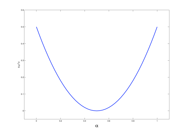
Figure 1: The measure $\frac{E(\varrho)^{2}}{2}$ for the mixed states in Example 4.1

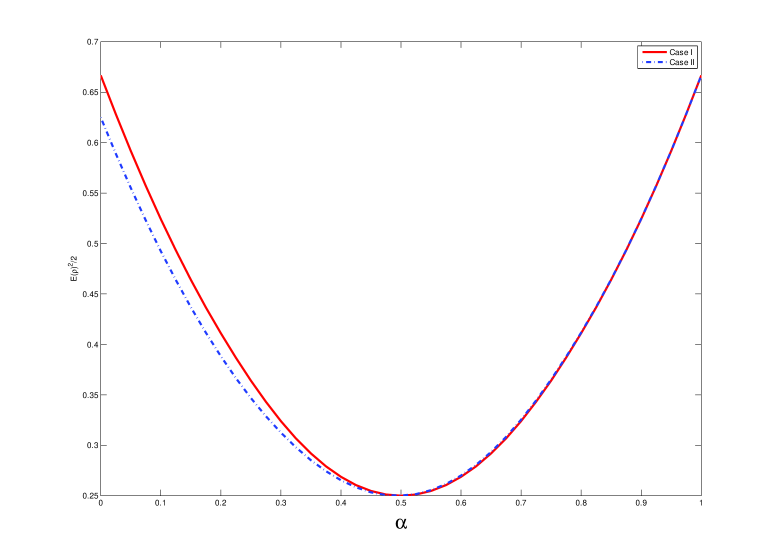
Figure 2: The measure $\frac{E(\varrho)^{2}}{2}$ for the mixed states in Example 4.2

5 Conclusion

We have extended the geometric measure to mixed states and established a characterization of the nearest disentangled mixed state of a given mixed state with respect to this measure. The analogue results for the quantum eigenvalue of a pure state are established for mixed states, i.e., Proposition 4.2 and Theorem 4.1. Based on this geometric measure, further works on the analysis and the computation are desired.

References

• [1] D.C. Brody and L.P. Hughston, Geometric quantum mechanics, J. Geom. Phys., 38, 19–53, 2001.
• [2] L. Chen, A. Xu and H. Zhu, Computation of the geometric measure of entanglement for pure multiqubit states, Phys. Rev. A, 82, 032301, 2010.
• [3] O. Gühne, F. Bodoky and M. Blaauboer, Multiparticle entanglement under the influence of decoherence, Phys. Rev. A, 78, 060301, 2008.
• [4] M. Hayashi, D. Markham, M. Murao, M. Owari and S. Virmani, The geometric measure of entanglement for a symmetric pure state with non-negative amplitudes, J. Math. Phys., 50, 122104, 2009.
• [5] J.J. Hilling and A. Sudbery, The geometric measure of multipartite entanglement and the singular values of a hypermatrix, J. Math. Phys., 51, 072102, 2010.
• [6] S. Hu, L. Qi and G. Zhang, The geometric measure of entanglement of pure states with nonnegative amplitudes and the spectral theory of nonnegative tensors, arXiv:1203.3675v5.
• [7] R. Hübener, M. Kleinmann, T.-C. Wei, C. G. Guillén, C. Gonzalez-Guillen and O. Gühne, Geometric measure of entanglement for symmetric states, Phys. Rev. A, 80, 032324, 2009.
• [8] D. Huybrechts, Complex Geometry: An Introduction, Springer, Berlin, 2005.
• [9] M.A. Nielsen and I.L. Chuang, Quantum Computing and Quantum Information, Cambridge University Press, Cambridge, 2000.
• [10] M.B. Plenio and S. Virmani, An introduction to entanglement measures, Quantum Inf. Comput., 7, 1–51, 2007.
• [11] L. Qi, The minimum Hartree value for the quantum entanglement problem, arXiv:1202.2983v1.
• [12] R.T. Rockafellar, Convex Analysis, Princeton Publisher, Princeton, 1970.
• [13] A. Sanpera, R. Tarrach and G. Vidal, Local description of quantum inseparability, Phys. Rev. A, 58, 826, 1998.
• [14] A. Shimony, Degree of entanglement, Ann. N. Y. Acad. Sci., 755, 675–679, 1995.
• [15] G. Vidal, Entanglement monotones, J. Mod. Opt., 47, 355–376, 2000.
• [16] T.C. Wei and P.M. Goldbart, Geometric measure of entanglement and applications to bipartite and multipartite quantum states, Phys. Rev. A, 68, 042307, 2003.
• [17] W.K. Wootters, Entanglement of formation of an arbitrary state of two qubits, Phys. Rev. Lett., 80, 2245, 1998.
• [18] T. Xiang, Density-matrix renormalization-group method in momentum space, Phys. Rev. B, 53, R10445, 1996.