Supervised Feature Selection in Graphs with Path Coding Penalties
and Network Flows

Abstract

We consider supervised learning problems where the features are embedded in a graph, such as gene expressions in a gene network. In this context, it is of much interest to automatically select a subgraph with few connected components; by exploiting prior knowledge, one can indeed improve the prediction performance or obtain results that are easier to interpret. Regularization or penalty functions for selecting features in graphs have recently been proposed, but they raise new algorithmic challenges. For example, they typically require solving a combinatorially hard selection problem among all connected subgraphs. In this paper, we propose computationally feasible strategies to select a sparse and well-connected subset of features sitting on a directed acyclic graph (DAG). We introduce structured sparsity penalties over paths on a DAG called “path coding” penalties. Unlike existing regularization functions that model long-range interactions between features in a graph, path coding penalties are tractable. The penalties and their proximal operators involve path selection problems, which we efficiently solve by leveraging network flow optimization. We experimentally show on synthetic, image, and genomic data that our approach is scalable and leads to more connected subgraphs than other regularization functions for graphs.

Keywords: convex and non-convex optimization, network flow optimization, graph sparsity

1 Introduction

Supervised sparse estimation problems have been the topic of much research in statistical machine learning and signal processing. In high dimensional settings, restoring a signal or learning a model is often difficult without a priori knowledge. When the solution is known beforehand to be sparse—that is, has only a few non-zero coefficients, regularizing with sparsity-inducing penalties has been shown to provide better prediction and solutions that are easier to interpret. For that purpose, non-convex penalties and greedy algorithms have been proposed (Akaike, 1973; Schwarz, 1978; Rissanen, 1978; Mallat and Zhang, 1993; Fan and Li, 2001). More recently, convex relaxations such as the $\ell_{1}$-norm (Tibshirani, 1996; Chen et al., 1999) and efficient algorithms have been developed (Osborne et al., 2000; Nesterov, 2007; Beck and Teboulle, 2009; Wright et al., 2009).

In this paper, we consider supervised learning problems where more information is available than just sparsity of the solution. More precisely, we assume that the features (or predictors) can be identified to the vertices of a graph, such as gene expressions in a gene network. In this context, it can be desirable to take into account the graph structure in the regularization (Rapaport et al., 2007). In particular, we are interested in automatically identifying a subgraph with few connected components (Jacob et al., 2009; Huang et al., 2011), groups of genes involved in a disease for example. There are two equally important reasons for promoting the connectivity of the problem solution: either connectivity is a prior information, which might improve the prediction performance, or connected components may be easier to interpret than isolated variables.

Formally, let us consider a supervised sparse estimation problem involving $p$ features, and let us assume that we are given an undirected or directed graph $G=(V,E)$, where $V$ is a vertex set identified to $\{1,\ldots,p\}$, and $E\subseteq V\times V$ is an arc (edge) set. Classical empirical risk minimization problems can be formulated as

$$\min_{{\mathbf{w}}\in{\mathbb{R}}^{p}}[L({\mathbf{w}})+\lambda\Omega({\mathbf{w}})],$$ (1)

where ${\mathbf{w}}$ is a weight vector in ${\mathbb{R}}^{p}$, which we wish to estimate; $L:{\mathbb{R}}^{p}\to{\mathbb{R}}$ is a convex loss function, and $\Omega:{\mathbb{R}}^{p}\to{\mathbb{R}}$ is a regularization function. In order to obtain a sparse solution, $\Omega$ is often chosen to be the $\ell_{0}$- (cardinality of the support) or $\ell_{1}$-penalty. In this paper, we are also interested in encouraging the sparsity pattern of ${\mathbf{w}}$ (the set of non-zero coefficients) to form a subgraph of $G$ with few connected components.

To the best of our knowledge, penalties promoting the connectivity of sparsity patterns in a graph can be classified into two categories. The ones of the first category involve pairwise interactions terms between vertices linked by an arc (Cehver et al., 2008; Jacob et al., 2009; Chen et al., 2011); each term encourages two neighbors in the graph to be simultaneously selected. Such regularization functions usually lead to tractable optimization problems, but they do not model long-range interactions between variables in the graph, and they do not promote large connected components. Penalties from the second category are more complex, and directly involve hard combinatorial problems (Huang et al., 2011). As such, they cannot be used without approximations. The problem of finding tractable penalties that model long-range interactions is therefore acute. The main contribution of our paper is a solution to this problem when the graph is directed and acyclic.

Of much interest to us are the non-convex penalty of Huang et al. (2011) and the convex penalty of Jacob et al. (2009). Given a pre-defined set of possibly overlapping groups of variables $\mathcal{G}$, these two structured sparsity-inducing regularization functions encourage a sparsity pattern to be in the union of a small number of groups from ${\mathcal{G}}$. Both penalties induce a similar regularization effect and are strongly related to each other. In fact, we show in Section 3 that the penalty of Jacob et al. (2009) can be interpreted as a convex relaxation of the non-convex penalty of Huang et al. (2011). These two penalties go beyond classical unstructured sparsity, but they are also complex and raise new challenging combinatorial problems. For example, Huang et al. (2011) define $\mathcal{G}$ as the set of all connected subgraphs of $G$, which leads to well-connected solutions but also leads to intractable optimization problems; the latter are approximately addressed by Huang et al. (2011) with greedy algorithms. Jacob et al. (2009) choose a different strategy and define $\mathcal{G}$ as the pairs of vertices linked by an arc, which, as a result, encourages neighbors in the graph to be simultaneously selected. This last formulation is computationally tractable, but does not model long-range interactions between features. Another suggestion from Jacob et al. (2009) and Huang et al. (2011) consists of defining $\mathcal{G}$ as the set of connected subgraphs up to a size $k$. The number of such subgraphs is however exponential in $k$, making this approach difficult to use even for small subgraph sizes ($k\!=\!3,4$) as soon as the graph is large ($p\!\approx\!10\,000$) and connected enough. These observations naturally raise the question: can we replace connected subgraphs by another structure that is rich enough to model long-range interactions in the graph and leads to computationally feasible penalties?

When the graph $G$ is directed and acyclic, we propose a solution built upon two ideas. First, we use in the penalty framework of Jacob et al. (2009) and Huang et al. (2011) a novel group structure $\mathcal{G}_{p}$ that contains all the paths in $G$; a path is defined as a sequence of vertices $(v_{1},\ldots,v_{k})$ such that for all $1\!\leq\!i<\!k$, we have $(v_{i},v_{i+1})\!\in\!E$. The second idea is to use appropriate costs for each path (the “price” one has to pay to select a path), which, as we show in the sequel, allows us to leverage network flow optimization. We call the resulting regularization functions “path coding” penalties. They go beyond pairwise interactions between vertices and model long-range interactions between the variables in the graph. They encourage sparsity patterns forming subgraphs that can be covered by a small number of paths, therefore promoting connectivity of the solution. We illustrate the “path coding” concept for DAGs in Figure 1. Even though the number of paths in a DAG is exponential in the graph size, we map the path selection problems our penalties involve to network flow formulations (see Ahuja et al., 1993; Bertsekas, 1998), which can be solved in polynomial time. As shown in Section 3, we build minimum cost flow formulations such that sending a positive amount of flow along a path for minimizing a cost is equivalent to selecting the path. This allows us to efficiently compute the penalties and their proximal operators, a key tool to address regularized problems (see Bach et al., 2012, for a review).

(a) Sparsity pattern in an undirected graph.

(b) Selected paths in a DAG.

Figure 1: Left LABEL:sub@subfig:undirected: an undirected graph. A sparsity pattern forming a subgraph with two connected components is represented by gray nodes. Right LABEL:sub@subfig:dag: when the graph is a DAG, the sparsity pattern is covered by two paths $(2,3,6)$ and $(9,11,12)$ represented by bold arrows.

Therefore, we make in this paper a new link between structured graph penalties in DAGs and network flow optimization. The development of network flow optimization techniques has been very active from the 60’s to the 90’s (see Ford and Fulkerson, 1956; Goldberg and Tarjan, 1986; Ahuja et al., 1993; Goldberg, 1997; Bertsekas, 1998). They have attracted a lot of attention during the last decade in the computer vision community for their ability to solve large-scale combinatorial problems typically arising in image segmentation tasks (Boykov et al., 2001). Concretely, by mapping a problem at hand to a network flow formulation, one can possibly obtain fast algorithms to solve the original problem. Of course, such a mapping does not always exist or can be difficult to find. This is made possible in the context of path coding penalties thanks to decomposability properties of the path costs, which we make explicit in Section 3.

We remark that different network flow formulations have also been used recently for sparse estimation (Cehver et al., 2008; Chambolle and Darbon, 2009; Hoefling, 2010; Mairal et al., 2011). Cehver et al. (2008) combine for example sparsity and Markov random fields for signal reconstruction tasks. They introduce a non-convex penalty consisting of pairwise interaction terms between vertices of a graph, and their approach requires iteratively solving maximum flow problems. It has also been shown by Chambolle and Darbon (2009) and Hoefling (2010) that for the anisotropic total-variation penalty, called “fused lasso” in statistics, the solution to problem (1) can be obtained by solving a sequence of parametric maximum flow problems. The total-variation penalty can be useful to obtain piecewise constant solutions on a graph (see Chen et al., 2011). Finally, Mairal et al. (2011) have shown that the structured sparsity-inducing regularization function of Jenatton et al. (2011) is related to network flows in a similar way as the total variation penalty. Note that both Jacob et al. (2009) and Jenatton et al. (2011) use the same terminology of “group Lasso with overlapping groups”, leading to some confusion in the literature. Yet, their works are significantly different and are in fact complementary: given a group structure ${\mathcal{G}}$, the penalty of Jacob et al. (2009) encourages solutions whose sparsity pattern is a union of a few groups, whereas the penalty of Jenatton et al. (2011) promotes an intersection of groups. It is natural to use the framework of Jacob et al. (2009) to encourage connectivity of a problem solution in a graph, e.g., by choosing ${\mathcal{G}}$ as the pairs of vertices linked by arc. It is however not obvious how to obtain this effect with the penalty of Jenatton et al. (2011). We discuss this question in more details in Appendix A.

To summarize, we have designed non-convex and convex penalty functions to do feature selection in directed acyclic graphs. Because our penalties involve an exponential number of variables, one for every path in the graph, existing optimization techniques cannot be used. To deal with this issue, we introduce network flow optimization tools that implicitly handle the exponential number of paths, allowing the penalties and their proximal operators to be computed in polynomial time. As a result, our penalties can model long-range interactions in the graph and are tractable.

The paper is organized as follows: In Section 2, we present preliminary tools, notably a brief introduction to network flows. In Section 3, we propose the path coding penalties and optimization techniques for solving the corresponding sparse estimation problems. Section 4 is devoted to experiments on synthetic, genomic, and image data to demonstrate the benefits of path coding penalties over existing ones and the scalability of our approach. Section 5 concludes the paper.

2 Preliminaries

As we show later, our path coding penalties are related to the concept of flow in a graph. Since this concept is not widely used in the machine learning literature, we provide a brief overview of this topic in Section 2.1. In Section 2.2, we also present proximal gradient methods, which have become very popular for solving sparse regularized problems (see Bach et al., 2012).

2.1 Network Flow Optimization

Network flows have been well studied in the computer science community, and have led to efficient dedicated algorithms for solving particular linear programs (see Ahuja et al., 1993; Bertsekas, 1998). Let us consider a directed graph $G\!=\!(V,E)$ with two special nodes $s$ and $t$, respectively dubbed source and sink. A flow $f$ on the graph $G$ is defined as a non-negative function on arcs $[f_{uv}]_{(u,v)\in E}$ that satisfies two sets of linear constraints:

• capacity constraints: the value of the flow $f_{uv}$ on an arc $(u,v)$ in $E$ should satisfy the constraint $l_{uv}\!\leq\!f_{uv}\!\leq\!\delta_{uv}$, where $l_{uv}$ and $\delta_{uv}$ are respectively called lower and upper capacities;

• conservation constraints: the sum of incoming flow at a vertex is equal to the sum of outgoing flow except for the source $s$ and the sink $t$.

We present examples of flows in Figures 2a and 2b, and denote by ${\mathcal{F}}$ the set of flows on a graph $G$. We remark that with appropriate graph transformations, the flow definition we have given admits several variants. It is indeed possible to consider several source and sink nodes, capacity constraints on the amount of flow going through vertices, or several arcs with different capacities between two vertices (see more details in Ahuja et al., 1993).

(a) A flow in a DAG.

(b) A flow in a directed graph with a cycle.

(c) $(s,t)$-path flow in a DAG.

(d) A cycle flow in a directed graph.

Figure 2: Examples of flows in a graph. LABEL:sub@subfig:flow1 The flow on the DAG can be interpreted as two units of flow sent from $s$ to $t$ along the paths $(s,1,3,4,t)$ and $(s,2,3,4,t)$. LABEL:sub@subfig:flow2 The flow can be interpreted as two units of flow sent from $s$ to $t$ on the same paths as in LABEL:sub@subfig:flow1 plus a unit of flow circulating along the cycle $(1,3,2,1)$. LABEL:sub@subfig:flow3 $(s,t)$-path flow along the path $(s,2,3,4,t)$. LABEL:sub@subfig:flow4 Cycle flow along $(1,3,2,1)$.

Some network flow problems have attracted a lot of attention because of their wide range of applications, for example in engineering, physics, transportation, or telecommunications (see Ahuja et al., 1993). In particular, the maximum flow problem consists of computing how much flow can be sent from the source to the sink through the network (Ford and Fulkerson, 1956). In other words, it consists of finding a flow $f$ in ${\mathcal{F}}$ maximizing $\sum_{u\in V:(s,u)\in E}f_{su}$. Another more general problem, which is of interest to us, is the minimum cost flow problem. It consists of finding a flow $f$ in ${\mathcal{F}}$ minimizing a linear cost $\sum_{(u,v)\in E}c_{uv}f_{uv}$, where every arc $(u,v)$ in $E$ has a cost $c_{uv}$ in ${\mathbb{R}}$. Both the maximum flow and minimum cost flow problems are linear programs, and can therefore be solved using generic linear programming tools, e.g., interior points methods (see Boyd and Vandenberghe, 2004; Nocedal and Wright, 2006). Dedicated algorithms exploiting the network structure of flows have however proven to be much more efficient. It has indeed been shown that minimum cost flow problems can be solved in strongly polynomial time—that is, an exact solution can be obtained in a finite number of steps that is polynomial in $|V|$ and $|E|$ (see Ahuja et al., 1993). More important, these dedicated algorithms are empirically efficient and can often handle large-scale problems (Goldberg and Tarjan, 1986; Goldberg, 1997; Boykov et al., 2001).

Among linear programs, network flow problems have a few distinctive features. The most striking one is the “physical” interpretation of a flow as a sum of quantities circulating in the network. The flow decomposition theorem (see Ahuja et al., 1993, Theorem 3.5) makes this interpretation more precise by saying that every flow vector can always be decomposed into a sum of $(s,t)$-path flows (units of flow sent from $s$ to $t$ along a path) and cycle flows (units of flow circulating along a cycle in the graph). We give examples of $(s,t)$-path and cycle flow in Figures 2c and 2d, and present examples of flows in Figures 2a and 2b along with their decompositions. Built upon the interpretation of flows as quantities circulating in the network, efficient algorithms have been developed, e.g., the classical augmenting path algorithm of Ford and Fulkerson (1956) for solving maximum flow problems. Another feature of flow problems is the locality of the constraints; each one only involves neighbors of a vertex in the graph. This locality is also exploited to design algorithms (Goldberg and Tarjan, 1986; Goldberg, 1997). Finally, minimum cost flow problems have a remarkable integrality property: a minimum cost flow problem where all capacity constraints are integers can be shown to have an integral solution (see Ahuja et al., 1993).

Later in our paper, we will map path selection problems to network flows by exploiting the flow decomposition theorem. In a nutshell, this apparently simple theorem has an interesting consequence: minimum cost flow problems can be seen from two equivalent viewpoints. Either one is looking for the value $f_{uv}$ of a flow on every arc $(u,v)$ of a graph minimizing the cost $\sum_{(u,v)\in E}c_{uv}f_{uv}$, or one is looking for the quantity of flow that should circulate on every $(s,t)$-path and cycle flow for minimizing the same cost. Of course, when the graph $G$ is a DAG, cycle flows do not exist. We will define flow problems such that selecting a path in the context of our path coding penalties is equivalent to sending some flow along a corresponding $(s,t)$-path. We will also exploit the integrality property to develop tools both adapted to non-convex penalties and convex ones, respectively involving discrete and continuous optimization problems. With these tools in hand, we will be able to deal efficiently with a simple class of optimization problems involving our path coding penalties. To deal with the more complex problem (1), we will need additional tools, which we now present.

2.2 Proximal Gradient Methods

Proximal gradient methods are iterative schemes for minimizing objective functions of the same form as (1), when the function $L$ is convex and differentiable with a Lipschitz continuous gradient. The simplest proximal gradient method consists of linearizing at each iteration the function $L$ around a current estimate ${\mathbf{\tilde{w}}}$, and this estimate is updated as the (unique by strong convexity) solution to

$$\min_{{\mathbf{w}}\in\mathbb{R}^{p}}\Big{[}\underbrace{L({\mathbf{\tilde{w}}})+\nabla L({\mathbf{\tilde{w}}})^{\top}({\mathbf{w}}-{\mathbf{\tilde{w}}})}_{\text{linear approximation of }L}+\underbrace{\frac{\rho}{2}\|{\mathbf{w}}-{\mathbf{\tilde{w}}}\|_{2}^{2}}_{\text{quadratic term}}+\underbrace{\lambda\Omega({\mathbf{w}})}_{\text{non-smooth part}}\Big{]},$$ (2)

which is assumed to be easier to solve than the original problem (1). The quadratic term keeps the update in a neighborhood where $L$ is close to its linear approximation, and the parameter $\rho$ is an upper bound on the Lipschitz constant of $\nabla L$. When $\Omega$ is convex, this scheme is known to converge to the solution to problem (1) and admits variants with optimal convergence rates among first-order methods (Nesterov, 2007; Beck and Teboulle, 2009). When $\Omega$ is non-convex, the guarantees are weak (finding the global optimum is out of reach), but it is easy to show that these updates can be seen as a majorization-minimization algorithm (Hunter and Lange, 2004) iteratively decreasing the value of the objective function (Wright et al., 2009; Mairal, 2013). When $\Omega$ is the $\ell_{1}$- or  $\ell_{0}$-penalty, the optimization schemes (2) are respectively known as iterative soft- and hard-thresholding algorithms (Daubechies et al., 2004; Blumensath and Davies, 2009). Note that when $L$ is not differentiable, similar schemes exist, known as mirror-descent (Nemirovsky and Yudin, 1983).

Another insight about these methods can be obtained by rewriting sub-problem (2) as

$$\min_{{\mathbf{w}}\in\mathbb{R}^{p}}\left[{\displaystyle\frac{1}{2}}\Big{\|}{\mathbf{\tilde{w}}}-\frac{1}{\rho}\nabla L({\mathbf{\tilde{w}}})-{\mathbf{w}}\Big{\|}_{2}^{2}+\frac{\lambda}{\rho}\Omega({\mathbf{w}})\right].$$

When $\lambda=0$, the solution is obtained by a classical gradient step ${\mathbf{\tilde{w}}}\leftarrow{\mathbf{\tilde{w}}}-(1/\rho)\nabla L({\mathbf{\tilde{w}}})$. Thus, proximal gradient methods can be interpreted as a generalization of gradient descent algorithms when dealing with a nonsmooth term. They are, however, only interesting when problem (2) can be efficiently solved. Formally, we wish to be able to compute the proximal operator defined as:

Definition 1 (Proximal Operator.)

The proximal operator associated with a regularization term $\lambda\Omega$, which we denote by $\text{Prox}_{\lambda\Omega}$, is the function that maps a vector ${\mathbf{u}}\in{\mathbb{R}}^{p}$ to the unique (by strong convexity) solution to

$$\min_{{\mathbf{w}}\in{\mathbb{R}}^{p}}\left[\frac{1}{2}\|{\mathbf{u}}-{\mathbf{w}}\|_{2}^{2}+\lambda\Omega({\mathbf{w}})\right].$$ (3)

Computing efficiently this operator has been shown to be possible for many penalties $\Omega$ (see Bach et al., 2012). We will show in the sequel that it is also possible for our path coding penalties.

3 Sparse Estimation in Graphs with Path Coding Penalties

We now present our path coding penalties, which exploit the structured sparsity frameworks of Jacob et al. (2009) and Huang et al. (2011). Because we choose a group structure $\mathcal{G}_{p}$ with an exponential number of groups, one for every path in the graph, the optimization techniques presented by Jacob et al. (2009) or Huang et al. (2011) cannot be used anymore. We will deal with this issue by introducing flow definitions of the path coding penalties.

3.1 Path Coding Penalties

The so-called “block coding” penalty of Huang et al. (2011) can be written for a vector ${\mathbf{w}}$ in ${\mathbb{R}}^{p}$ and any set $\mathcal{G}$ of groups of variables as

$$\varphi_{{\mathcal{G}}}({\mathbf{w}})\triangleq\min_{{\mathcal{J}}\subseteq{\mathcal{G}}}\Big{\{}\sum_{g\in{\mathcal{J}}}\eta_{g}~{}~{}\text{s.t.}~{}~{}\text{Supp}({\mathbf{w}})\subseteq\bigcup_{g\in{\mathcal{J}}}g\Big{\}},$$ (4)

where the $\eta_{g}$’s are non-negative weights, and ${\mathcal{J}}$ is a subset of groups in ${\mathcal{G}}$ whose union covers the support of ${\mathbf{w}}$ formally defined as $\text{Supp}({\mathbf{w}})\triangleq\{j\in\{1,\ldots,p\}:{\mathbf{w}}_{j}\neq 0\}$. When the weights $\eta_{g}$ are well chosen, the non-convex penalty $\varphi_{{\mathcal{G}}}$ encourages solutions ${\mathbf{w}}$ whose support is in the union of a small number of groups; in other words, the cardinality of ${\mathcal{J}}$ should be small. We remark that Huang et al. (2011) originally introduce this regularization function under a more general information-theoretic point of view where $\varphi_{{\mathcal{G}}}$ is a code length (see Barron et al., 1998; Cover and Thomas, 2006), and the weights $\eta_{g}$ represent the number of bits encoding the fact that a group $g$ is selected. One motivation for using $\varphi_{{\mathcal{G}}}$ is that the selection of a few groups might be easier to interpret than the selection of isolated variables. This formulation extends non-convex group sparsity regularization by allowing any group structure ${\mathcal{G}}$ to be considered. Nevertheless, a major drawback is that computing this non-convex penalty $\varphi_{{\mathcal{G}}}({\mathbf{w}})$ for a general group structure $\mathcal{G}$ is difficult. Equation (4) is indeed an instance of a set cover problem, which is NP-hard (see Cormen et al., 2001), and appropriate approximations, e.g., greedy algorithms, have to be used in practice.

As often when dealing with non-convex penalties, one can either try to solve directly the corresponding non-convex problems or look for a convex relaxation. As we empirically show in Section 4, having both non-convex and convex variants of a penalty can be a significant asset. One variant can indeed outperform the other one in some situations, while being the other way around in some other cases. It is therefore interesting to look for a convex relaxation of $\varphi_{{\mathcal{G}}}$. We denote by $\eta$ the vector $[\eta_{g}]_{g\in{\mathcal{G}}}$ in ${\mathbb{R}}_{+}^{|{\mathcal{G}}|}$, and by ${\mathbf{N}}$ the binary matrix in $\{0,1\}^{p\times|{\mathcal{G}}|}$ whose columns are indexed by the groups $g$ in ${\mathcal{G}}$, such that the entry ${\mathbf{N}}_{jg}$ is equal to one when the index $j$ is in the group $g$, and zero otherwise. Equation (4) can be rewritten as a Boolean linear program, a form which will be more convenient in the rest of the paper:

$$\varphi_{{\mathcal{G}}}({\mathbf{w}})=\min_{{\mathbf{x}}\in\{0,1\}^{|{\mathcal{G}}|}}\left\{\eta^{\top}{\mathbf{x}}~{}~{}\text{s.t.}~{}~{}{\mathbf{N}}{\mathbf{x}}\geq\text{Supp}({\mathbf{w}})\right\},$$ (5)

where, with an abuse of notation, $\text{Supp}({\mathbf{w}})$ is here a vector in $\{0,1\}^{p}$ such that its $j$-th entry is $1$ if $j$ is in the support of ${\mathbf{w}}$ and $0$ otherwise. Let us also denote by $|{\mathbf{w}}|$ the vector in ${\mathbb{R}}_{+}^{p}$ obtained by replacing the entries of ${\mathbf{w}}$ by their absolute value. We can now consider a convex relaxation of $\varphi_{{\mathcal{G}}}$:

$$\psi_{{\mathcal{G}}}({\mathbf{w}})\triangleq\min_{{\mathbf{x}}\in{\mathbb{R}}_{+}^{|{\mathcal{G}}|}}\left\{\eta^{\top}{\mathbf{x}}~{}~{}\text{s.t.}~{}~{}{\mathbf{N}}{\mathbf{x}}\geq|{\mathbf{w}}|\right\},$$ (6)

where not only the optimization problem above is a linear program, but in addition $\psi_{{\mathcal{G}}}$ is a convex function—in fact it can be shown to be a norm. Such a relaxation is classical and corresponds to the same mechanism relating the $\ell_{0}$- to the $\ell_{1}$-penalty, replacing $\text{Supp}({\mathbf{w}})$ by $|{\mathbf{w}}|$. The next lemma tells us that we have in fact obtained a variant of the penalty introduced by Jacob et al. (2009).

Lemma 1 (Relation Between $\psi_{{\mathcal{G}}}$ and the Penalty of Jacob et al. (2009).)

Suppose that any pattern in $\{0,1\}^{p}$ can be represented by a union of groups in ${\mathcal{G}}$. Then, the function $\psi_{{\mathcal{G}}}$ defined in (6) is equal to the penalty of Jacob et al. (2009) with $\ell_{\infty}$-norms.

Note that Jacob et al. (2009) have introduced their penalty from a different perspective, and the link between (6) and their work is not obvious at first sight. In addition, their penalty involves a sum of $\ell_{2}$-norms, which needs to be replaced by $\ell_{\infty}$-norms for the lemma to hold. Hence, $\psi_{{\mathcal{G}}}$ is a “variant” of the penalty of Jacob et al. (2009). We give more details and the proof of this lemma in Appendix B.

Now that $\varphi_{{\mathcal{G}}}$ and $\psi_{{\mathcal{G}}}$ have been introduced, we are interested in automatically selecting a small number of connected subgraphs from a directed acyclic graph $G=(V,E)$. In Section 1, we already discussed group structures $\mathcal{G}$ and introduced $\mathcal{G}_{p}$ the set of paths in $G$. As a result, the path coding penalties $\varphi_{{\mathcal{G}}_{p}}$ and ${\psi}_{{{\mathcal{G}}}_{p}}$ encourage solutions that are sparse while forming a subgraph that can be covered by a small number of paths. As we show in this section, this choice leads to tractable formulations when the weights $\eta_{g}$ for every path $g$ in $\mathcal{G}_{p}$ are appropriately chosen.

We will show in the sequel that a natural choice is to define for all $g$ in $\mathcal{G}_{p}$

$$\eta_{g}\triangleq\gamma+|g|,$$ (7)

where $\gamma$ is a new parameter encouraging the connectivity of the solution whereas $|g|$ encourages sparsity. It is indeed possible to show that when $\gamma\!=\!0$, the functions $\varphi_{{\mathcal{G}}_{p}}$ and ${\psi}_{{{\mathcal{G}}}_{p}}$ respectively become the $\ell_{0}$- and the $\ell_{1}$-penalties, therefore encouraging sparsity but not connectivity. On the other hand, when $\gamma$ is large and the term $|g|$ is negligible, $\varphi_{{\mathcal{G}}_{p}}({\mathbf{w}})$ simply “counts” how many paths are required to cover the support of ${\mathbf{w}}$, thereby encouraging connectivity regardless of the sparsity of ${\mathbf{w}}$.

In fact, the choice (7) is a particular case of a more general class of weights $\eta_{g}$, which our algorithmic framework can handle. Let us enrich the original directed acyclic graph $G$ by introducing a source node $s$ and a sink node $t$. Formally, we define a new graph $G^{\prime}=(V^{\prime},E^{\prime})$ with

$$\begin{split}V^{\prime}&\triangleq V\cup\{s,t\},\\ E^{\prime}&\triangleq E\cup\{(s,v):v\in V\}\cup\{(u,t):u\in V\}.\end{split}$$

In plain words, the graph $G^{\prime}$, which is a DAG, contains the graph $G$ and two nodes $s,t$ that are linked to every vertices of $G$. Let us also assume that some costs $c_{uv}$ in ${\mathbb{R}}$ are defined for all arcs $(u,v)$ in $E^{\prime}$. Then, for a path $g=(u_{1},u_{2},\ldots,u_{k})$ in $\mathcal{G}_{p}$, we define the weight $\eta_{g}$ as

$$\eta_{g}\triangleq c_{su_{1}}+\Big{(}\sum_{i=1}^{k-1}c_{u_{i}u_{i+1}}\Big{)}+c_{u_{k}t}=\sum_{(u,v)\in(s,g,t)}c_{uv},$$ (8)

where the notation $(s,g,t)$ stands for the path $(s,u_{1},u_{2},\ldots,u_{k},t)$ in $G^{\prime}$. The decomposition of the weights $\eta_{g}$ as a sum of costs on $(s,t)$-paths of $G^{\prime}$ (the paths $(s,g,t)$ with $g$ in $\mathcal{G}_{p}$) is a key component of the algorithmic framework we present next. The construction of the graph $G^{\prime}$ is illustrated in Figures 3a and 3b for two cost configurations. We remark that the simple choice of weights (7) corresponds to the choice (8) with the costs $c_{su}=\gamma$ for all $u$ in $V$ and $c_{uv}=1$ otherwise (see Figure 3a). Designing costs $c_{uv}$ that go beyond the simple choice (7) can be useful whenever one has additional knowledge about the graph structure. For example, we experimentally exploit this property in Section 4.2 to privilege or penalize paths $g$ in ${\mathcal{G}}_{p}$ starting from a particular vertex. This is illustrated in Figure 3b where the cost on the arc $(s,1)$ is much smaller than on the arcs $(s,2)$, $(s,3)$, $(s,4)$, therefore encouraging paths starting from vertex $1$.

Another interpretation connecting the path-coding penalties with coding lengths and random walks can be drawn using information theoretic arguments derived from Huang et al. (2011). We find these connections interesting, but for simplicity only present them in Appendix C. In the next sections, we address the following issues: (i) how to compute the penalties $\varphi_{{\mathcal{G}}_{p}}$ and ${\psi}_{{{\mathcal{G}}}_{p}}$ given a vector ${\mathbf{w}}$ in ${\mathbb{R}}^{p}$? (ii) how to optimize the objective function (1)? (iii) in the convex case (when $\Omega={\psi}_{{{\mathcal{G}}}_{p}}$), can we obtain practical optimality guarantees via a duality gap? All of these questions will be answered using network flow and convex optimization, or algorithmic tools on graphs.

(a) Graph $G^{\prime}$ with arcs costs and a path $g$ in bold red.

(b) Graph $G^{\prime}$ with different arcs costs and a path $g$.

Figure 3: LABEL:sub@subfig:grapha $G^{\prime}$ is obtained by adding a source $s$ and sink $t$ to a DAG with four nodes. The cost configuration is such that the weights $\eta_{g}$ satisfy $\eta_{g}=\gamma+|g|$. For example, for $g=(4,2,3)$, the sum of costs along $(s,g,t)$ is $\eta_{g}=\gamma+3$. LABEL:sub@subfig:graphb Same graph $G^{\prime}$ as LABEL:sub@subfig:grapha but with different costs. The weight $\eta_{g}$ associated to the path $g=(1,2)$ is the sum of costs along $(s,1,2,t)$—that is, $\eta_{g}=4$.

3.2 Flow Definitions of the Path Coding Penalties

Before precisely stating the flow definitions of $\varphi_{{\mathcal{G}}_{p}}$ and ${\psi}_{{{\mathcal{G}}}_{p}}$, let us sketch the main ideas. The first key component is to transform the optimization problems (4) and (6) over the paths in $G$ into optimization problems over $(s,t)$-path flows in $G^{\prime}$. We recall that $(s,t)$-path flows are defined as flow vectors carrying the same positive value on every arc of a path between $s$ and $t$. It intuitively corresponds to sending from $s$ to $t$ a positive amount of flow along a path, an interpretation we have presented in Figure 2 from Section 2.1. Then, we use the flow decomposition theorem (see Section 2.1), which provides two equivalent viewpoints for solving a minimum cost flow problem on a DAG. One should be either looking for the value $f_{uv}$ of a flow on every arc $(u,v)$ of the graph, or one should decide how much flow should be sent on every $(s,t)$-path.

We assume that a cost configuration $[c_{uv}]_{(u,v)\in E^{\prime}}$ is available and that the weights $\eta_{g}$ are defined according to Equation (8). We denote by ${\mathcal{F}}$ the set of flows on $G^{\prime}$. The second key component of our approach is the fact that the cost of a flow $f$ in ${\mathcal{F}}$ sending one unit from $s$ to $t$ along a path $g$ in $G$, defined as $\sum_{(u,v)\in E^{\prime}}f_{uv}c_{uv}=\sum_{(u,v)\in(s,g,t)}c_{uv}$ is exactly $\eta_{g}$, according to Equation (8). This enables us to reformulate our optimization problems (4) and (6) on paths in $G$ as optimization problems on $(s,t)$-path flows in $G^{\prime}$, which in turn are equivalent to minimum cost flow problems and can be solved in polynomial time. Note that this equivalence does not hold when we have cycle flows (see Figure 2d), and this is the reason why we have assumed $G$ to be acyclic.

We can now formally state the mappings between the penalties $\varphi_{{\mathcal{G}}_{p}}$ and ${\psi}_{{{\mathcal{G}}}_{p}}$ on one hand, and network flows on the other hand. An important quantity in the upcoming propositions is the amount of flow going through a vertex $j$ in $V\!=\!\{1,\ldots,p\}$, which we denote by

$$s_{j}(f)\triangleq\sum_{u\in V^{\prime}:(u,j)\in E^{\prime}}f_{uj}.$$

Our formulations involve capacity constraints and costs for $s_{j}(f)$, which can be handled by network flow solvers; in fact, a vertex can always be equivalently replaced in the network by two vertices, linked by an arc that carries the flow quantity $s_{j}(f)$ (Ahuja et al., 1993). The main propositions are presented below, and the proofs are given in Appendix D.

Proposition 1 (Computing $\varphi_{{\mathcal{G}}_{p}}$.)

Let ${\mathbf{w}}$ be in ${\mathbb{R}}^{p}$. Consider the network $G^{\prime}$ defined in Section 3.1 with costs $[c_{uv}]_{(u,v)\in E^{\prime}}$, and define $\eta_{g}$ as in (8). Then,

$$\varphi_{{\mathcal{G}}_{p}}({\mathbf{w}})=\min_{f\in{\mathcal{F}}}\left\{\sum_{(u,v)\in E^{\prime}}f_{uv}c_{uv}~{}~{}\text{s.t.}~{}~{}s_{j}(f)\geq 1,~{}\forall j\in\text{Supp}({\mathbf{w}})\right\},$$ (9)

where ${\mathcal{F}}$ is the set of flows on $G^{\prime}$. This is a minimum cost flow problem with some lower-capacity constraints, which can be computed in strongly polynomial time.

Given the definition of the penalty $\varphi_{{\mathcal{G}}}$ in Eq. (5), computing $\varphi_{{\mathcal{G}}_{p}}$ seems challenging for two reasons: (i) Eq. (5) is for a general group structure $\mathcal{G}$ a NP-hard Boolean linear program with $|\mathcal{G}|$ variables; (ii) the size of $\mathcal{G}_{p}$ is exponential in the graph size. Interestingly, Proposition 1 tells us that these two difficulties can be overcome when $\mathcal{G}=\mathcal{G}_{p}$ and that the non-convex penalty $\varphi_{{\mathcal{G}}_{p}}$ can be computed in polynomial time by solving the convex optimization problem defined in Eq. (9). The key component to obtain the flow definition of $\varphi_{{\mathcal{G}}_{p}}$ is the decomposability property of the weights $\eta_{g}$ defined in (8). This allows us to identify the cost of sending one unit of flow in $G^{\prime}$ from $s$ to $t$ along a path $g$ to the cost of selecting the path $g$ in the context of the path coding penalty $\varphi_{{\mathcal{G}}_{p}}$. We now show that the same methodology applies to the convex penalty ${\psi}_{{{\mathcal{G}}}_{p}}$.

Proposition 2 (Computing ${\psi}_{{{\mathcal{G}}}_{p}}$.)

Let ${\mathbf{w}}$ be in ${\mathbb{R}}^{p}$. Consider the network $G^{\prime}$ defined in Section 3.1 with costs $[c_{uv}]_{(u,v)\in E^{\prime}}$, and define $\eta_{g}$ as in (8). Then,

$${\psi}_{{{\mathcal{G}}}_{p}}({\mathbf{w}})=\min_{f\in{\mathcal{F}}}\left\{\sum_{(u,v)\in E^{\prime}}f_{uv}c_{uv}~{}~{}\text{s.t.}~{}~{}s_{j}(f)\geq|{\mathbf{w}}_{j}|,~{}\forall j\in\{1,\ldots,p\}\right\},$$ (10)

where ${\mathcal{F}}$ is the set of flows on $G^{\prime}$. This is a minimum cost flow problem with some lower-capacity constraints, which can be computed in strongly polynomial time.

From the similarity between Equations (9) and (10), it is easy to see that ${\psi}_{{{\mathcal{G}}}_{p}}$ and $\varphi_{{\mathcal{G}}_{p}}$ are closely related, one being a convex relaxation of the other as explained in Section 3.1. We have shown here that $\varphi_{{\mathcal{G}}_{p}}$ and ${\psi}_{{{\mathcal{G}}}_{p}}$ can be computed in polynomial time and will discuss in Section 3.4 practical algorithms to do it in practice. Before that, we address the problem of optimizing (1).

3.3 Using Proximal Gradient Methods with the Path Coding Penalties

To address the regularized problem (1), we use proximal gradient methods, which we have presented in Section 2.2. We need for that to compute the proximal operators of $\varphi_{{\mathcal{G}}_{p}}$ and ${\psi}_{{{\mathcal{G}}}_{p}}$ from Definition 1. We show that this operator can be efficiently computed by using network flow optimization.

Proposition 3 (Computing the Proximal Operator of ${\varphi_{{\mathcal{G}}_{p}}}$.)

Let ${\mathbf{u}}$ be in ${\mathbb{R}}^{p}$. Consider the network $G^{\prime}$ defined in Section 3.1 with costs $[c_{uv}]_{(u,v)\in E^{\prime}}$, and define $\eta_{g}$ as in (8). Let us define

$$f^{\star}\in\operatornamewithlimits{arg\,min}_{f\in{\mathcal{F}}}\left\{\sum_{(u,v)\in E^{\prime}}f_{uv}c_{uv}+\sum_{j=1}^{p}\frac{1}{2}\max\left({\mathbf{u}}_{j}^{2}(1-s_{j}(f)),0\right)\right\},$$ (11)

where ${\mathcal{F}}$ is the set of flows on $G^{\prime}$. This is a minimum cost flow problem, with piecewise linear costs, which can be computed in strongly polynomial time. Denoting by ${\mathbf{w}}^{\star}\!\triangleq\!\text{Prox}_{\varphi_{{\mathcal{G}}_{p}}}[{\mathbf{u}}]$, we have for all $j$ in $V=\{1,\ldots,p\}$ that ${\mathbf{w}}^{\star}_{j}={\mathbf{u}}_{j}$ if $s_{f}(f^{\star})\!>\!0$ and $0$ otherwise.

Note that even though the formulation (3) is non-convex when $\Omega$ is the function $\varphi_{{\mathcal{G}}_{p}}$, its global optimum can be found by solving the convex problem described in Equation (11). As before, the key component to establish the mapping to a network flow problem is the decomposability property of the weights $\eta_{g}$. More details are provided in the proofs of Appendix D. Note also that any minimum cost flow problem with convex piecewise linear costs can be equivalently recast as a classical minimum cost flow problem with linear costs (see Ahuja et al., 1993), and therefore the above problem can be solved in strongly polynomial time. We now present similar results for ${\psi}_{{{\mathcal{G}}}_{p}}$.

Proposition 4 (Computing the Proximal Operator of ${{\psi}_{{{\mathcal{G}}}_{p}}}$.)

Let ${\mathbf{u}}$ be in ${\mathbb{R}}^{p}$. Consider the network $G^{\prime}$ defined in Section 3.1 with costs $[c_{uv}]_{(u,v)\in E^{\prime}}$, and define $\eta_{g}$ as in (8). Let us define

$$f^{\star}\in\operatornamewithlimits{arg\,min}_{f\in{\mathcal{F}}}\left\{\sum_{(u,v)\in E^{\prime}}f_{uv}c_{uv}+\sum_{j=1}^{p}\frac{1}{2}\max\big{(}|{\mathbf{u}}_{j}|-s_{j}(f),0\big{)}^{2}\right\},$$ (12)

where ${\mathcal{F}}$ is the set of flows on $G^{\prime}$. This is a minimum cost flow problem, with piecewise quadratic costs, which can be computed in polynomial time. Denoting by ${\mathbf{w}}^{\star}\!\triangleq\!\text{Prox}_{{\psi}_{{{\mathcal{G}}}_{p}}}[{\mathbf{u}}]$, we have for all $j$ in $V\!=\!\{1,\ldots,p\}$, ${\mathbf{w}}^{\star}_{j}=\operatorname{sign}({\mathbf{u}}_{j})\min(|{\mathbf{u}}_{j}|,s_{j}(f^{\star}))$.

The proof of this proposition is presented in Appendix D. We remark that we are dealing in Proposition 4 with a minimum cost flow problem with quadratic costs, which is more difficult to solve than when the costs are linear. Such problems with quadratic costs can be solved in weakly (instead of strongly) polynomial time (see Hochbaum, 2007)—that is, a time polynomial in $|V|$, $|E|$ and $\log(\|{\mathbf{u}}\|_{\infty}/\varepsilon)$ to obtain an $\varepsilon$-accurate solution to problem (12), where $\varepsilon$ can possibly be set to the machine precision. We have therefore shown that the computations of $\varphi_{{\mathcal{G}}_{p}}$, ${\psi}_{{{\mathcal{G}}}_{p}}$, $\text{Prox}_{\varphi_{{\mathcal{G}}_{p}}}$ and $\text{Prox}_{{\psi}_{{{\mathcal{G}}}_{p}}}$ can be done in polynomial time. We now discuss practical algorithms, which have empirically shown to be efficient and scalable (Goldberg, 1997; Bertsekas, 1998).

3.4 Practical Algorithms for Solving the Network Flow Problems

The minimum cost flow problems involved in the computations of $\varphi_{{\mathcal{G}}_{p}}$, ${\psi}_{{{\mathcal{G}}}_{p}}$ and $\text{Prox}_{\varphi_{{\mathcal{G}}_{p}}}$ can be solved in the worst-case with $O\big{(}(|V|\log|V|)(|E|+|V|\log|V|)\big{)}$ operations (see Ahuja et al., 1993). However, this analysis corresponds to the worst-case possible and the empirical complexity of network flow solvers is often much better (Boykov et al., 2001). Instead of a strongly polynomial algorithm, we have chosen to implement the scaling push-relabel algorithm Goldberg (1997), also known as an $\varepsilon$-relaxation method (Bertsekas, 1998). This algorithm is indeed empirically efficient despite its weakly polynomial worst-case complexity. It requires transforming the capacities and costs of the minimum cost flow problems into integers with an appropriate scaling and rounding procedure, and denoting by $C$ the (integer) value of the maximum cost in the network its worst-case complexity is $O\big{(}|V|^{2}|E|\log(C|V|)\big{)}$. This algorithm is appealing because of its empirical efficiency when the right heuristics are used Goldberg (1997). We choose $C$ to be as large as possible (using $64$ bits integers) not to lose numerical precision, even though choosing $C$ according to the desired statistical precision and the robustness of the proximal gradient algorithms would be more appropriate. It has indeed been shown recently by Schmidt et al. (2011) that proximal gradient methods for convex optimization are robust to inexact computations of the proximal operator, as long as the precision of these computations iteratively increases with an appropriate rate.

Computing the proximal operator $\text{Prox}_{{\psi}_{{{\mathcal{G}}}_{p}}}[{\mathbf{u}}]$ requires dealing with piecewise quadratic costs, which are more complicated to deal with than linear costs. Fortunately, cost scaling or $\varepsilon$-relaxation techniques can be modified to handle any convex costs, while keeping a polynomial complexity (Bertsekas, 1998). Concisely describing $\varepsilon$-relaxation algorithms is difficult because their convergence properties do not come from classical convex optimization theory. We present here an interpretation of these methods, but we refer the reader to Chapter 9 of Bertsekas (1998) for more details and implementation issues. In a nutshell, consider a primal convex cost flow problem $\min_{f\in{\mathcal{F}}}\sum_{(u,v)\in E}C_{uv}(f_{uv})$, where the functions $C_{uv}$ are convex, and without capacity constraints. Using classical Lagrangian duality, it is possible to obtain the following dual formulation

$$\max_{\pi\in{\mathbb{R}}^{p}}\sum_{(u,v)\in E}q_{uv}(\pi_{u}-\pi_{v}),~{}~{}\text{where}~{}~{}q_{uv}(\pi_{u}-\pi_{v})\triangleq\min_{f_{uv}\geq 0}\left[C_{uv}(f_{uv})-(\pi_{u}-\pi_{v})f_{uv}\right].$$

This formulation is unconstrained and involves for each node $u$ in $V$ a dual variable $\pi_{u}$ in ${\mathbb{R}}$, which is called the price of node $u$. $\varepsilon$-relaxation techniques rely on this dual formulation, and can be interpreted as approximate dual coordinate ascent algorithms. They exploit the network structure to perform computationally cheap updates of the dual and primal variables, and can deal with the fact that the functions $q_{uv}$ are concave but not differentiable in general. Presenting how this is achieved exactly would be too long for this paper; we instead refer the reader to Chapter 9 of Bertsekas (1998). In the next section, we introduce algorithms to compute the dual norm of ${\psi}_{{{\mathcal{G}}}_{p}}$, which is an important quantity to obtain optimality guarantees for (1) with $\Omega={\psi}_{{{\mathcal{G}}}_{p}}$, or for implementing active set methods that are adapted to very large-scale very sparse problems (see Bach et al., 2012).

3.5 Computing the Dual-Norm of ${\psi}_{{{\mathcal{G}}}_{p}}$

The dual norm ${\psi}_{{{\mathcal{G}}}_{p}}^{*}$ of the norm ${\psi}_{{{\mathcal{G}}}_{p}}$ is defined for any vector ${\boldsymbol{\kappa}}$ in $\mathbb{R}^{p}$ as ${\psi}_{{{\mathcal{G}}}_{p}}^{*}({\boldsymbol{\kappa}})\triangleq\max_{{\psi}_{{{\mathcal{G}}}_{p}}({\mathbf{w}})\leq 1}{\mathbf{w}}^{\top}{\boldsymbol{\kappa}}$ (see Boyd and Vandenberghe, 2004). We show in this section that ${\psi}_{{{\mathcal{G}}}_{p}}^{*}$ can be computed efficiently.

Proposition 5 (Computing the Dual Norm ${\psi}_{{{\mathcal{G}}}_{p}}^{*}$.)

Let ${\boldsymbol{\kappa}}$ be in ${\mathbb{R}}^{p}$. Consider the network $G^{\prime}$ defined in Section 3.1 with costs $[c_{uv}]_{(u,v)\in E^{\prime}}$, and define $\eta_{g}$ as in (8). For $\tau\geq 0$, and all $j$ in $\{1,\ldots,p\}$, we define an additional cost for the vertex $j$ to be $-|{\boldsymbol{\kappa}}_{j}|/\tau$. We then define for every path $g$ in ${\mathcal{G}}_{p}$, the length $l_{\tau}(g)$ to be the sum of the costs along the corresponding $(s,t)$-path from $G^{\prime}$. Then,

$${\psi}_{{{\mathcal{G}}}_{p}}^{*}({\boldsymbol{\kappa}})=\min_{\tau\in{\mathbb{R}}_{+}}\left\{\tau~{}~{}\text{s.t.}~{}~{}\min_{g\in{\mathcal{G}}_{p}}l_{\tau}(g)\geq 0\right\},$$

and ${\psi}_{{{\mathcal{G}}}_{p}}^{*}({\boldsymbol{\kappa}})$ is the smallest factor $\tau$ such that the shortest $(s,t)$-path on $G^{\prime}$ has nonnegative length.

The proof is given in Appendix D. We note that the above quantity $l_{\tau}(g)$ satisfies $l_{\tau}(g)=\eta_{g}-\|{\boldsymbol{\kappa}}_{g}\|_{1}/\tau$, for every $\tau>0$ and ${\boldsymbol{\kappa}}$ in ${\mathbb{R}}^{p}$. We present a simple way for computing ${\psi}_{{{\mathcal{G}}}_{p}}^{*}$ in Algorithm 1, which is proven in Proposition 6 to be correct and to converge in polynomial time.

Algorithm 1 Computation of the Dual Norm ${\psi}_{{{\mathcal{G}}}_{p}}^{*}$.

0:  ${\boldsymbol{\kappa}}\in\mathbb{R}^{p}$ such that ${\boldsymbol{\kappa}}\neq 0$.

1:  Choose any path $g\in{\mathcal{G}}_{p}$ such that ${\boldsymbol{\kappa}}_{g}\neq 0$;

2:  $\delta\leftarrow-\infty$;

3:  while  $\delta<0$ do

4:     $\tau\leftarrow\frac{\|{\boldsymbol{\kappa}}_{g}\|_{1}}{\eta_{g}}$;

5:     $g\leftarrow\operatornamewithlimits{arg\,min}_{h\in{\mathcal{G}}_{p}}l_{\tau}(h)$; (shortest path problem in a directed acyclic graph);

6:     $\delta\leftarrow l_{\tau}(g)$;

7:  end while

8:  Return: $\tau={\psi}_{{{\mathcal{G}}}_{p}}^{*}({\boldsymbol{\kappa}})$ (value of the dual norm).

Proposition 6 (Correctness and Complexity of Algorithm 1.)

For ${\boldsymbol{\kappa}}$ in ${\mathbb{R}}^{p}$, the algorithm 1 computes ${\psi}_{{{\mathcal{G}}}_{p}}^{*}({\boldsymbol{\kappa}})$ in at most $O(p|E^{\prime}|)$ operations.

The proof is also presented in Appendix D. We note that this worst-case complexity bound might be loose. We have indeed observed in our experiments that the empirical complexity is close to be linear in $|E^{\prime}|$. To concretely illustrate why computing the dual norm can be useful, we now give optimality conditions for problem (1) involving ${\psi}_{{{\mathcal{G}}}_{p}}^{*}$. The following lemma can immediately be derived from Bach et al. (2012, Proposition 1.2).

Lemma 2 (Optimality Conditions for Problem (1) with $\Omega=\psi_{{\mathcal{G}}}$.)

A vector ${\mathbf{w}}$ be in ${\mathbb{R}}^{p}$ is optimal for problem (1) with $\Omega=\psi_{{\mathcal{G}}}$ if and only if

$$\psi_{{\mathcal{G}}}^{*}(\nabla L({\mathbf{w}}))\leq\lambda~{}~{}~{}\text{and}~{}~{}~{}-\nabla L({\mathbf{w}})^{\top}{\mathbf{w}}=\lambda\psi_{{\mathcal{G}}}({\mathbf{w}}).$$

The next section presents an active-set type of algorithm (see Bach et al., 2012, Chapter 6) building upon these optimality conditions and adapted to our penalty ${\psi}_{{{\mathcal{G}}}_{p}}$.

3.6 Active Set Methods for Solving Problem (1) when $\Omega={\psi}_{{{\mathcal{G}}}_{p}}$

As experimentally shown later in Section 4, proximal gradient methods allows us to efficiently solve medium-large/scale problems ($p<100\,000$). Solving larger scale problems can, however, be more difficult. Algorithm 2 is an active-set strategy that can overcome this issue when the solution is very sparse. It consists of solving a sequence of smaller instances of Equation (1) on subgraphs $\tilde{G}=(\tilde{V},\tilde{E})$, with $\tilde{V}\subseteq V$ and $\tilde{E}\subseteq E$, which we call active graphs. It is based on the computation of the dual-norm ${\psi}_{{{\mathcal{G}}}_{p}}^{*}$, which we have observed can empirically be obtained in a time linear or close to linear in $|E^{\prime}|$. Given such a subgraph $\tilde{G}$, we denote by $\tilde{{\mathcal{G}}}_{p}$ the set of paths in $\tilde{G}$. The subproblems the active set strategy involve are the following:

$$\min_{{\mathbf{w}}\in{\mathbb{R}}^{p}}\big{\{}L({\mathbf{w}})+\lambda{\psi}_{\tilde{{\mathcal{G}}}_{p}}({\mathbf{w}})~{}~{}\text{s.t.}~{}~{}{\mathbf{w}}_{j}=0~{}~{}\text{for all}~{}j\notin\tilde{V}\big{\}}.$$ (13)

The key observations are that (i) when $\tilde{G}$ is small, subproblem (13) is easy to solve; (ii) after solving (13), one can check optimality conditions for problem (1) using Lemma 2, and update $\tilde{G}$ accordingly. Algorithm 2 presents the full algorithm, and the next proposition ensures that it is correct.

Algorithm 2 Active-set Algorithm for Solving Equation (1) with $\Omega={\psi}_{{{\mathcal{G}}}_{p}}$.

1:  Initialization ${\mathbf{w}}\leftarrow 0$; $\tilde{G}\leftarrow(\emptyset,\emptyset)$ (active graph);

2:  loop

3:     Update ${\mathbf{w}}$ by solving subproblem (13) (using the current value of ${\mathbf{w}}$ as a warm start);

4:     Compute $\tau\leftarrow{\psi}_{{{\mathcal{G}}}_{p}}^{*}(\nabla L({\mathbf{w}}))$ (using Algorithm 1);

5:     if $\tau\leq\lambda$ then

6:        exit the loop;

7:     else

8:        $g\leftarrow\operatornamewithlimits{arg\,min}_{g\in{\mathcal{G}}_{p}}l_{\tau}(g)$ (shortest path problem in a directed acyclic graph);

9:        $\tilde{V}\leftarrow\tilde{V}\cup g$; $\tilde{E}\leftarrow\tilde{E}\cup\{(u,v)\in E:u\in g~{}~{}\text{and}~{}~{}v\in g\}$ (update of the active graph);

10:     end if

11:  end loop

12:  Return: ${\mathbf{w}}^{\star}\leftarrow{\mathbf{w}}$, solution to Equation (1).

Proposition 7 (Correctness of Algorithm 2.)

Algorithm 2 solves Equation (1) when $\Omega={\psi}_{{{\mathcal{G}}}_{p}}$.

The proof is presented in Appendix D. It mainly relies on Lemma 2, which requires computing the quantity ${\psi}_{{{\mathcal{G}}}_{p}}^{*}(\nabla L({\mathbf{w}}))$. More precisely, it can be shown that when ${\mathbf{w}}$ is a solution to subproblem (13) for a subgraph $\tilde{G}$, whenever ${\psi}_{{{\mathcal{G}}}_{p}}^{*}(\nabla L({\mathbf{w}}))\leq\lambda$, it is also a solution to the original large problem (1). Note that variants of Algorithm 2 can be considered: one can select more than a single path $g$ to update the subgraph $\tilde{G}$, or one can approximately solve the subproblems (13). In the latter case, the stopping criterion could be relaxed in practice. One could use the criterion $\tau\leq\lambda+\varepsilon$, where $\varepsilon$ is a small positive constant, or one could use a duality gap to stop the optimization when the solution is guaranteed to be optimal enough.

In the next section, we present various experiments, illustrating how the different penalties and algorithms behave in practice.

4 Experiments and Applications

We now present experiments on synthetic, genomic and image data. Our algorithms have been implemented in C++ with a Matlab interface, they have been made available as part of the open-source software package SPAMS, originally accompanying Mairal et al. (2010). We have implemented the proximal gradient algorithm FISTA (Beck and Teboulle, 2009) for convex regularization functions and ISTA for non-convex ones. When available, we use a relative duality gap as a stopping criterion and stop the optimization when the relative duality gap is smaller than $10^{-4}$. In our experiments, we often need to solve Equation (1) for several values of the parameter $\lambda$, typically chosen on a logarithmic grid. We proceed with a continuation strategy: first we solve the problem for the largest value of $\lambda$, whose solution can be shown to be $0$ when $\lambda$ is large enough; then we decrease the value of $\lambda$, and use the previously obtained solution as initialization. This warm-restart strategy allows us to quickly follow a regularization path of the problem. For non-convex problems, it provides us with a good initialization for a given $\lambda$. The algorithm ISTA with the non-convex penalty $\varphi_{{\mathcal{G}}_{p}}$ is indeed only guaranteed to iteratively decrease the value of the objective function. As often the case with non-convex problems, the quality of the optimization is subject to a good initialization, and this strategy has proven to be important to obtain good results.

As far as the choice of the parameters is concerned, we have observed that all penalties we have considered in our experiments are very sensitive to the regularization parameter $\lambda$. Thus, we use in general a fine grid to choose $\lambda$ using cross-validation or a validation set. Some of the penalties involve an extra parameter, $\gamma$ in the case of $\varphi_{{\mathcal{G}}_{p}}$ and ${\psi}_{{{\mathcal{G}}}_{p}}$. This parameter offers some flexibility, for example it promotes the connectivity of the solution for $\varphi_{{\mathcal{G}}_{p}}$ and ${\psi}_{{{\mathcal{G}}}_{p}}$, but it also requires to be tuned correctly to prevent overfitting. In practice, we have found the choice of the second parameter always less critical than $\lambda$ to obtain a good prediction performance, and thus we use a coarse grid to choose this parameter. All other implementation details are provided in each experimental section.

4.1 Synthetic Experiments

In this first experiment, we study our penalties $\varphi_{{\mathcal{G}}_{p}}$ and ${\psi}_{{{\mathcal{G}}}_{p}}$ in a controlled setting. Since generating synthetic graphs reflecting similar properties as real-life networks is difficult, we have considered three “real” graphs of different sizes, which are part of the 10${}^{\text{th}}$ DIMACS graph partitioning and graph clustering challenge:

• the graph jazz was compiled by Gleiser and Danon (2003) and represents a community network of jazz musicians. It contains $p=198$ vertices and $m=2\,742$ edges;

• the graph email was compiled by Guimerà et al. (2003) and represents e-mail exchanges in a university. It contains $p=1\,133$ vertices and $m=5\,451$ edges;

• the graph PGP was compiled by Boguñá et al. (2004) and represents information interchange among users in a computer network. It contains $p=10\,680$ vertices and $m=24\,316$ edges.

We choose an arbitrary topological ordering for all of these graphs, orient the arcs according to this ordering, and obtain DAGs. We generate structured sparse linear models with measurements corrupted by noise according to different scenarii, and compare the ability of different regularization functions to recover the noiseless model. More precisely, we consider a design matrix ${\mathbf{X}}$ in ${\mathbb{R}}^{n\times p}$ with less observations than predictors ($n\triangleq\lfloor p/2\rfloor$), and whose entries are i.i.d. samples from a normal distribution ${\mathcal{N}}(0,1)$. For simplicity, we preprocess each column of ${\mathbf{X}}$ by removing its mean component and normalize it to have unit $\ell_{2}$-norm. Then, we generate sparse vectors ${\mathbf{w}}_{0}$ with $k$ non-zero entries, according to different strategies described in the sequel. We synthesize an observation vector ${\mathbf{y}}={\mathbf{X}}{\mathbf{w}}_{0}+{\boldsymbol{\varepsilon}}$ in ${\mathbb{R}}^{n}$, where the entries of ${\boldsymbol{\varepsilon}}$ are i.i.d. draws from a normal distribution ${\mathcal{N}(0,\sqrt{k/n}\sigma)}$, with different noise levels:

• high SNR: we choose $\sigma=0.2$; this yields a signal noise ratio (SNR) $\|{\mathbf{X}}{\mathbf{w}}_{0}\|_{2}^{2}/\|{\boldsymbol{\varepsilon}}\|_{2}^{2}$ of about $26$. We note that for $\sigma\leq 0.1$ almost all penalties almost perfectly recover the true pattern;

• medium SNR: for $\sigma=0.4$, the SNR is about $6$;

• low SNR: for $\sigma=0.8$, the SNR is about $1.6$.

Choosing a good criterion for comparing different penalties is difficult, and a conclusion drawn from an experiment is usually only valid for a given criterion. For example, we present later an image denoising experiment in Section 4.2, where non-convex penalties outperform convex ones according to one performance measure, while being the other way around for another one. In this experiment, we choose the relative mean square error $\|{\mathbf{X}}{\bf\hat{w}}-{\mathbf{X}}{\mathbf{w}}_{0}\|_{2}^{2}$ as a criterion, and use ordinary least square (OLS) to refit the models learned using the penalties. Whereas OLS does not change the results obtained with the non-convex penalties we consider, it changes significantly the ones obtained with the convex ones. In practice, OLS counterbalances the “shrinkage” effect of convex penalties, and empirically improves the results quality for low noise regimes (high SNR), but deteriorates it for high noise regimes (low SNR).

For simplicity, we also assume (in this experiment only) that an oracle gives us the optimal regularization parameter $\lambda$, and therefore the conclusions we draw from the experiment are only the existence or not of good solutions on the regularization path for every penalty. A more exhaustive comparison would require testing different combinations (with OLS, without OLS) and different criteria, and using internal cross-validation to select the regularization parameters. This would require a much heavier computational setting, which we have chosen not to implement in this experiment. After obtaining the matrix ${\mathbf{X}}$, we propose several strategies to generate “true” models ${\mathbf{w}}_{0}$:

• in the scenario flat we randomly select $k$ entries without exploiting the graph structure;

• the scenario graph consists of randomly selecting $5$ entries, and iteratively selecting new vertices that are connected in $G$ to at least one previously selected vertex. This produces fairly connected sparsity patterns, but does not exploit arc directions;

• the scenario path is similar to graph, but we iteratively add new vertices following single paths in $G$. It exploits arc directions and produces sparsity patterns that can be covered by a small number of paths, which is the sort of patterns that our path-coding penalties encourage.

The number of non-zero entries in ${\mathbf{w}}_{0}$ is chosen to be $k\triangleq\lfloor 0.1p\rfloor$ for the different graphs, resulting in a fairly sparse vector. The values of the non-zero entries are randomly chosen in $\{-1,+1\}$. We consider the formulation (1) where $L$ is the square loss: $L({\mathbf{w}})=\frac{1}{2}\|{\mathbf{y}}-{\mathbf{X}}{\mathbf{w}}\|_{2}^{2}$ and $\Omega$ is one of the following penalties:

• the classical $\ell_{0}$- and $\ell_{1}$-penalties;

• the penalty $\psi_{{\mathcal{G}}}$ of Jacob et al. (2009) where the groups $\mathcal{G}$ are pairs of vertices linked by an arc;

• our path-coding penalties $\varphi_{{\mathcal{G}}_{p}}$ or ${\psi}_{{{\mathcal{G}}}_{p}}$ with the weights $\eta_{g}$ defined in (7).

• the penalty of Huang et al. (2011), and their strategy to encourage sparsity pattern with a small number of connected components. We use their implementation of the greedy algorithm StructOMP. This algorithm uses a strategy dubbed “block-coding” to approximately deal with this penalty (see Huang et al., 2011), and has an additional parameter, which we also denote by $\mu$, to control the trade-off between sparsity and connectivity.

For every method except StructOMP, the regularization parameter $\lambda$ is chosen among the values $2^{i/4}$, where $i$ is an integer. We always start from a large value for $i$, and decrease its value by one, following the regularization path. For the penalties $\varphi_{{\mathcal{G}}_{p}}$ and ${\psi}_{{{\mathcal{G}}}_{p}}$, the parameter $\gamma$ is simply chosen in $\{1/4,1/2,1,2,4\}$. Since the algorithm StructOMP is greedy and iteratively increases the model complexity, we record every solution obtained on the regularization path during one pass of the algorithm. Based on information-theoretic arguments, Huang et al. (2011) propose a default value for their parameter $\mu=1$. Since changing this parameter value empirically improves the results quality, we try the values $\{1/4,1/2,1,2,4\}$ for a fair comparison with our penalties $\varphi_{{\mathcal{G}}_{p}}$ and ${\psi}_{{{\mathcal{G}}}_{p}}$.

We report the results for the three graphs, three scenarii for generating ${\mathbf{w}}_{0}$, three noise levels and the five penalties in Figure 4. We report on these graphs the ratio between the prediction mean square error and the best achievable error if the sparsity pattern was given by an oracle. In other words, denoting by ${\bf\hat{w}}^{\text{oracle}}$ the OLS estimate if an oracle gives us the sparsity pattern, we report the value $\|{\mathbf{X}}{\bf\hat{w}}-{\mathbf{X}}{\mathbf{w}}_{0}\|_{2}^{2}/\|{\mathbf{X}}{\bf\hat{w}}^{\text{oracle}}-{\mathbf{X}}{\mathbf{w}}_{0}\|_{2}^{2}$. The best achievable value for this criterion is therefore $1$, which is represented by a dotted line on all graphs. We reproduce the experiment $20$ times, randomizing every step, including the way the vector ${\mathbf{w}}_{0}$ is generated to obtain error bars representing one standard deviation.

We make pairwise comparisons and statistically assess our conclusions using error bars or, when needed, paired one-sided T-tests with a $1\%$ significance level. The comparisons are the following:

• convex vs non-convex ($\ell_{0}$ vs $\ell_{1}$ and $\varphi_{{\mathcal{G}}_{p}}$ vs ${\psi}_{{{\mathcal{G}}}_{p}}$): For high SNR, non-convex penalties do significantly better than convex ones, whereas it is the other way around for low SNR. The differences are highly significant for the graphs email and PGP. For medium SNR, conclusions are mixed, either the difference between a convex penalty and its non-convex counterpart are not significant or one is better than another.

• unstructured vs path-coding ($\ell_{0}$ vs $\varphi_{{\mathcal{G}}_{p}}$ and $\ell_{1}$ vs ${\psi}_{{{\mathcal{G}}}_{p}}$): In the structured scenarii graph and path, the structured penalties $\varphi_{{\mathcal{G}}_{p}}$ and ${\psi}_{{{\mathcal{G}}}_{p}}$ respectively do better than $\ell_{0}$ and $\ell_{1}$. In the unstructured flat scenario, $\ell_{0}$ and $\ell_{1}$ should be preferred. More precisely, for the scenarii graph and path, $\varphi_{{\mathcal{G}}_{p}}$ and ${\psi}_{{{\mathcal{G}}}_{p}}$ respectively outperform $\ell_{0}$ and $\ell_{1}$ with statistically significant differences, except (i) for high SNR, both $\varphi_{{\mathcal{G}}_{p}}$ and $\ell_{0}$ achieve perfect recovery; (ii) with the smallest graph jazz, the $p$-values obtained to compare ${\psi}_{{{\mathcal{G}}}_{p}}$ vs $\ell_{1}$ are slightly above our $1\%$ significance level. In the flat scenario, $\ell_{0}$ and $\varphi_{{\mathcal{G}}_{p}}$ give similar results, whereas ${\psi}_{{{\mathcal{G}}}_{p}}$ performs slightly worse than $\ell_{1}$ in general even though they are very close.

• Jacob et al. (2009) vs path-coding ($\psi_{{\mathcal{G}}}$ with pairs vs ${\psi}_{{{\mathcal{G}}}_{p}}$): in the scenario path, ${\psi}_{{{\mathcal{G}}}_{p}}$ outperforms $\psi_{{\mathcal{G}}}$ (pairs). It is generally also the case in the scenario graph. The differences are always significant in the low SNR regime and with the largest graph PGP.

• Huang et al. (2011) vs path-coding (StructOMP vs $\varphi_{{\mathcal{G}}_{p}},{\psi}_{{{\mathcal{G}}}_{p}}$): For the scenario path, either $\varphi_{{\mathcal{G}}_{p}}$ (for high SNR) or ${\psi}_{{{\mathcal{G}}}_{p}}$ (for low SNR) outperform StructOMP. For the scenario graph, the best results are shared between StructOMP and our penalties for high and medium SNR, and our penalties do better for low SNR. More precisely in the scenario graph: (i) there is no significant difference for high SNR between $\varphi_{{\mathcal{G}}_{p}}$ and StructOMP; (ii) for medium SNR, StructOMP does slightly better with the graph PGP and similarly as $\varphi_{{\mathcal{G}}}$ for the two other graphs; (iii) for low SNR, our penalties do better than StructOMP with the two largest graphs email and PGP and similarly with the smallest graph jazz.

To conclude this experiment, we have shown that our penalties offer a competitive alternative to StructOMP and the penalty of Jacob et al. (2009), especially when the “true” sparsity pattern is exactly a union of a few paths in the graph. We have also identified different noise and size regimes, where a penalty should be preferred to another. Our experiment also shows that having both a non-convex and convex variant of a penalty can be interesting. In low SNR, convex penalties are indeed better behaved than non-convex ones, whereas it is the other way around when the SNR is high.

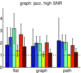
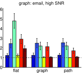
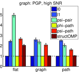
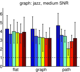
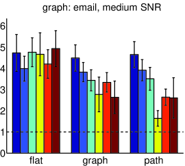
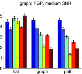
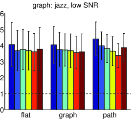
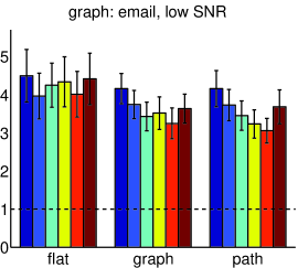
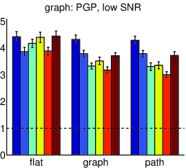
Figure 4: Every bar represents the ratio between the mean square error estimate and the oracle mean square error estimate (see main text for an explicit formula and the full experimental setting). The error bars represent one standard deviation. Each row corresponds to a specific noise level, and every column to a different graph. For a specific noise level and specific graph, the results for three scenarii, flat, graph and path are reported. Each group of six bars represents the results obtained with six penalties, from left to right: $\ell_{0}$, $\ell_{1}$, $\psi_{{\mathcal{G}}}$ (with $\mathcal{G}$ being the pairs of vertices linked by an arc), $\varphi_{{\mathcal{G}}_{p}}$, ${\psi}_{{{\mathcal{G}}}_{p}}$, and the method StructOMP. A legend is presented in the top right figure.

4.2 Image Denoising

State-of-the-art image restoration techniques are often exploiting a good model for small image patches (Elad and Aharon, 2006; Dabov et al., 2007; Mairal et al., 2009). We consider here the task of denoising natural images corrupted by white Gaussian noise, following an approach introduced by Elad and Aharon (2006). It consists of the following steps:

1. extract all overlapping patches $({\mathbf{y}}^{i})_{i=1,\ldots,m}$ from a noisy image;

2. compute a sparse approximation of every individual patch ${\mathbf{y}}^{i}$:

   $$\min_{{\mathbf{w}}^{i}\in{\mathbb{R}}^{p}}\Big{[}\frac{1}{2}\|{\mathbf{y}}^{i}-{\mathbf{X}}{\mathbf{w}}^{i}\|_{2}^{2}+\lambda\Omega({\mathbf{w}}^{i})\Big{]},$$ (14)

   where the matrix ${\mathbf{X}}=[{\mathbf{x}}^{1},\ldots,{\mathbf{x}}^{p}]$ in ${\mathbb{R}}^{n\times p}$ is a predefined “dictionary”, $\lambda\Omega$ is a sparsity-inducing regularization and the term ${\mathbf{X}}{\mathbf{w}}^{i}$ is the clean estimate of the noisy patch ${\mathbf{y}}^{i}$;

3. since the patches overlap, each pixel admits several estimates. The last step consists of averaging the estimates of each pixel to reconstruct the full image.

Whereas Elad and Aharon (2006) learn an overcomplete basis set to obtain a “good” matrix ${\mathbf{X}}$ in the step 2 above, we choose a simpler approach and use a classical orthogonal discrete cosine transform (DCT) dictionary ${\mathbf{X}}$ (Ahmed et al., 1974). We present such a dictionary in Figure 5 for $8\times 8$ image patches. As shown in the figure, DCT elements can be organized on a two-dimensional grid and ordered by horizontal and vertical frequencies. We use the DAG structure connecting neighbors on the grid, going from low to high frequencies. In this experiment, we address the following questions:

• In terms of optimization, is our approach efficient for this experiment? Because the number of problems to solve is large (several millions), the task is difficult.

• Do we get better results by using the graph structure than with classical $\ell_{0}$- and $\ell_{1}$-penalties?

• How does the method compare with the state of the art?

Figure 5: Orthogonal DCT dictionary with $n=8\times 8$ image patches. The dictionary elements are organized by horizontal and vertical frequencies.

Note that since the dictionary ${\mathbf{X}}$ in ${\mathbb{R}}^{n\times p}$ is orthogonal, the non-convex problems we address here are solved exactly. Indeed, it can be shown that Equation (14) is equivalent to

$$\min_{{\mathbf{w}}^{i}\in{\mathbb{R}}^{p}}\Big{[}\frac{1}{2}\|{\mathbf{X}}^{\top}{\mathbf{y}}^{i}-{\mathbf{w}}^{i}\|_{2}^{2}+\lambda\Omega({\mathbf{w}}^{i})\Big{]},$$

and therefore the solution admits a closed form ${\mathbf{w}}^{i\star}\!\triangleq\!\text{Prox}_{\lambda\Omega}({\mathbf{X}}^{\top}{\mathbf{y}}^{i})$. For $\ell_{0}$ and $\ell_{1}$, the solution is respectively obtained by hard and soft-thresholding, and we have introduced some tools in Section 3 to compute the proximal operators of $\varphi_{{\mathcal{G}}_{p}}$ and ${\psi}_{{{\mathcal{G}}}_{p}}$. We consider $e\times e$ image patches, with $e\in\{6,8,10,12,14,16\}$, and a parameter $\lambda$ on a logarithmic scale with step $2^{1/8}$. We also exploit the variant of our penalties presented in Section 3 that allows us to choose the costs on the arcs of the graph $G^{\prime}$. We choose here a small cost on the arc $(s,1)$ of the graph $G^{\prime}$, and a large one for every arc $(s,j)$, for $j$ in $\{2,\ldots,p\}$, such that all paths selected by our approach are encouraged to start by the variable $1$ (equivalently the dictionary element ${\mathbf{x}}^{1}$ with the lowest frequencies). We use a dataset of $12$ classical high-quality images (uncompressed and free of artifact). We optimize the parameters $\lambda$ and $e$ on the first $3$ images, keeping the $9$ last images as a test set and report denoising results on Table 1. Even though this dataset is relatively small, it is standard in the image processing literature, making the comparison easy with other approaches.

We start by answering question (A): we have observed that the time of computation depends on several factors, including the problem size and the sparsity of the solution (the sparser, the faster). In the setting $\sigma\!=\!10$ and $e\!=\!8$, we are able to denoise approximately $4\,000$ patches per second using $\varphi_{{\mathcal{G}}_{p}}$, and $1\,800$ in the setting $\sigma\!=\!50$ and $e\!=\!14$ with our laptop 1.2Ghz CPU (core i3 330UM). The penalty ${\psi}_{{{\mathcal{G}}}_{p}}$ requires solving quadratic minimum cost flow problems, and is slower to use in practice: the numbers $4\,000$ and $1\,800$ above respectively become $70$ and $130$. Our approach with $\varphi_{{\mathcal{G}}_{p}}$ proves therefore to be fairly efficient for our task, allowing us to process an image with about $250\,000$ patches in between one and three minutes. As expected, simple penalties are faster to use: about $65\,000$ patches per second can be processed using $\ell_{0}$.

Moving to question (B), the best performance among the penalties $\ell_{0}$, $\ell_{1}$, $\varphi_{{\mathcal{G}}_{p}}$ and ${\psi}_{{{\mathcal{G}}}_{p}}$ is obtained by $\varphi_{{\mathcal{G}}_{p}}$. This difference is statistically significant: we measure for instance an average improvement of $0.38\pm 0.21$ dB over $\ell_{0}$ for $\sigma\geq 20$. For this denoising task, it is indeed typical to have non-convex penalties outperforming convex ones (see Mairal, 2010, Section 1.6.5, for a benchmark between $\ell_{0}$ and $\ell_{1}$-penalties), and this is why the original method of Elad and Aharon (2006) uses the $\ell_{0}$-penalty. Interestingly, this superiority of non-convex penalties in this denoising scheme based on overlapping patches is usually only observed after the averaging step 3. When one evaluates the quality of the denoising of individual patches without averaging—that is, after step 2, opposite conclusions are usually drawn (see again Mairal, 2010, Section 1.6.5). We therefore report mean-square error results for individual patches without averaging in Table 2 when $e=10$. As expected, the penalty ${\psi}_{{{\mathcal{G}}}_{p}}$ turns out to be the best at this stage of the algorithm. Note that the bad results obtained by convex penalties after the averaging step are possibly due to the shrinkage effect of these penalties. It seems that the shrinkage is helpful for denoising individual patches, but hurts after the averaging process.

We also present the performance of state-of-the-art image denoising approaches in Table 1 to address question (C). We have chosen to include in the comparison several methods that have successively been considered as the state of the art in the past: the Gaussian Scale Mixture (GSM) method of Portilla et al. (2003), the K-SVD algorithm of Elad and Aharon (2006), the BM3D method of Dabov et al. (2007) and the sparse coding approach of Mairal et al. (2009) (LSSC). We of course do not claim to do better than the most recent approaches of Dabov et al. (2007) or Mairal et al. (2009), which in addition to sparsity exploit non-local self similarities in images (Buades et al., 2005). Nevertheless, given the fact that we use a simple orthogonal DCT dictionary, unlike Elad and Aharon (2006) who learn overcomplete dictionaries adapted to the image, our approach based on the penalty $\varphi_{{\mathcal{G}}_{p}}$ performs relatively well. We indeed obtain similar results as Elad and Aharon (2006) and Portilla et al. (2003), and show that structured parsimony could be a promising tool in image processing.

$\sigma$	5	10	15	20	25	50	100
Our approach
$\ell_{0}$	37.04	33.15	31.03	29.59	28.48	25.26	22.44
$\ell_{1}$	36.42	32.28	30.06	28.59	27.51	24.48	21.96
$\varphi_{{\mathcal{G}}_{p}}$	37.01	33.22	31.21	29.82	28.77	25.73	22.97
${\psi}_{{{\mathcal{G}}}_{p}}$	36.32	32.17	29.99	28.54	27.49	24.54	22.12
State-of-the-art approaches
Portilla et al., 2003 (GSM)	36.96	33.19	31.17	29.78	28.74	25.67	22.96
Elad and Aharon, 2006 (K-SVD)	37.11	33.28	31.22	29.81	28.72	25.29	22.02
Dabov et al., 2007 (BM3D)	37.24	33.60	31.68	30.36	29.36	26.11	23.11
Mairal et al., 2009 (LSSC)	37.29	33.64	31.70	30.36	29.33	26.20	23.20

Table 1: Denoising results for $9$ test images. The numbers represent the average PSNR in dB (higher is better). Denoting by MSE the mean-squared-error for images whose intensities are between $0$ and $255$, the PSNR is defined as $\textrm{PSNR}=10\log_{10}(255^{2}/\textrm{MSE})$. Pixel values are scaled between $0$ and $255$ and $\sigma$ (the standard deviation of the noise) is between $5$ and $100$. The top part of the table presents the results of the denoising scheme obtained with different penalties. The bottom part presents the results obtained with various state-of-the-art denoising methods (see main text for more details). Best results are in bold for both parts of the table.

$\sigma$	5	10	15	20	25	50	100
$\ell_{0}$	3.60	10.00	16.65	23.22	29.58	57.97	95.79
$\ell_{1}$	2.68	7.65	13.42	19.22	25.23	52.38	87.90
$\varphi_{{\mathcal{G}}_{p}}$	3.26	8.36	13.62	18.83	23.99	47.66	84.74
${\psi}_{{{\mathcal{G}}}_{p}}$	2.66	7.27	12.29	17.35	22.65	45.04	76.85

Table 2: Denoising results for individual $10\times 10$ image patches on the $9$ test images. The numbers represent the mean-squared error for the image patches (lower the better). Best results are in bold.

4.3 Breast Cancer Data

One of our goal was to develop algorithmic tools improving the approach of Jacob et al. (2009). It is therefore natural to try one of the dataset they used to obtain an empirical comparison. On the one hand, we have developed tools to enrich the group structure that the penalty $\psi_{{\mathcal{G}}}$ could handle, and thus we expect better results. On the other hand, the graph in this experiment is undirected and we need to use heuristics to transform it into a DAG.

We use in this task the breast cancer dataset of Van De Vijver et al. (2002). It consists of gene expression data from $8\,141$ genes in $n\!=\!295$ breast cancer tumors and the goal is to classify metastatic samples versus non-metastatic ones. Following Jacob et al. (2009), we use the gene network compiled by Chuang et al. (2007), obtained by concatenating several known biological networks. As argued by Jacob et al. (2009), taking into account the graph structure into the regularization has two objectives: (i) possibly improving the prediction performance by using a better prior; (ii) identifying connected subgraphs of genes that might be involved in the metastatic form of the disease, leading to results that yield better interpretation than the selection of isolated genes. Even though prediction is our ultimate goal in this task, interpretation is equally important since it is necessary in practice to design drug targets. In their paper, Jacob et al. (2009) have succeeded in the sense that their penalty is able to extract more connected patterns than the $\ell_{1}$-regularization, even though they could not statistically assess significant improvements in terms of prediction. Following Jacob et al. (2009), we also assume that connectivity of the solution is an asset for interpretation. The questions we address here are the following:

• Despite the heuristics described below to transform the graph into a DAG, does our approach lead to well-connected solutions in the original (undirected) graph? Do our penalties lead to better-connected solutions than other penalties?.

• Do our penalties lead to better classification performance than Jacob et al. (2009) and other classical unstructured and structured regularization functions? Is the graph structure useful to improve the prediction? Does sparsity help prediction?

• How efficient is our approach for this task? The problem here is of medium/large scale but should be solved a large number of times (several thousands of times) because of the internal cross-validation procedure.

The graph of genes, which we denote by $G_{0}$, contains $42\,587$ edges, and, like Jacob et al. (2009), we keep the $p\!=\!7\,910$ genes that are present in $G_{0}$. In order to obtain interpretable results and select connected components of $G_{0}$, Jacob et al. (2009) use their structured sparsity penalty $\psi_{{\mathcal{G}}}$ where the groups $\mathcal{G}$ are all pairs of genes linked by an arc. Our approach requires a DAG, but we will show in the sequel that we nevertheless obtain good results after heuristically transforming $G_{0}$ into a DAG. To do so, we first treat $G_{0}$ as directed by choosing random directions on the arcs, and second we remove some arcs along cycles in the graph. It results in a DAG containing $33\,303$ arcs, which we denote by $G$. This pre-processing step is of course questionable since our penalties are originally not designed to deal with the graph $G_{0}$. We of course do not claim to be able to individually interpret each path selected by our method, but, as we show, it does not prevent our penalties $\varphi_{{\mathcal{G}}_{p}}$ and ${\psi}_{{{\mathcal{G}}}_{p}}$ to achieve their ultimate goal—that is connectivity in the original graph $G_{0}$.

We consider the formulation (1) where $L$ is a weighted logistic regression loss:

$$L({\mathbf{w}})\triangleq\sum_{i=1}^{n}\frac{1}{n_{y_{i}}}\log(1+e^{-y_{i}{\mathbf{w}}^{\top}{\mathbf{x}}_{i}}),$$

where the $y_{i}$’s are labels in $\{-1,+1\}$, the ${\mathbf{x}}_{i}$’s are gene expression vectors in ${\mathbb{R}}^{p}$. The weight $n_{1}$ is the number of positive samples, whereas $n_{-1}$ the number of negative ones. This model does not include an intercept, but the gene expressions are centered. The regularization functions included in the comparison are the following:

• our path-coding penalties $\varphi_{{\mathcal{G}}_{p}}$ and ${\psi}_{{{\mathcal{G}}}_{p}}$ with the weights $\eta_{g}$ defined in (7);

• the squared $\ell_{2}$-penalty (ridge logistic regression);

• the $\ell_{1}$-norm (sparse logistic regression);

• the elastic-net penalty of Zou and Hastie (2005), which has the form ${\mathbf{w}}\to\|{\mathbf{w}}\|_{1}+(\mu/2)\|{\mathbf{w}}\|_{2}^{2}$, where $\mu$ is an additional parameter;

• the penalty $\psi_{{\mathcal{G}}}$ of Jacob et al. (2009) where the groups $\mathcal{G}$ are pairs of vertices linked by an arc;

• a variant of the penalty $\psi_{{\mathcal{G}}}$ of Jacob et al. (2009) whose form is given in Equation (16) of Appendix B, where the $\ell_{2}$-norm is used in place of the $\ell_{\infty}$-norm;

• the penalty $\zeta_{\mathcal{G}}$ of Jenatton et al. (2011) given in Appendix A where the groups are all pairs of vertices linked by an arc;

• the penalty $\zeta_{\mathcal{G}}$ of Jenatton et al. (2011) using the group structure adapted to DAGs described in Appendix A. This penalty has shown to be empirically problematic to use directly. The number of groups each variable belongs to significantly varies from a variable to another, resulting in overpenalization for some variables and underpenalization for some others. To cope with this issue, we have tried different strategies to choose the weights $\eta_{g}$ for every group in the penalty, similarly as those described by Jenatton et al. 2011, but we have been unable to obtain sparse solutions in this setting (typically the penalty selects here more than a thousand variables). A heuristic that has proven to be much better is to add a weighted $\ell_{1}$-penalty to $\zeta_{\mathcal{G}}$ to correct the over/under-penalization issue. Denoting for a variable $j$ in $\{1,\ldots,p\}$ by $d_{j}$ the number of groups the variable $j$ belongs to—in other words $d_{j}\triangleq\sum_{g\in\mathcal{G}:g\ni j}1$, we add the term $\sum_{j=1}^{p}(\max_{k}d_{k}-d_{j})|{\mathbf{w}}_{j}|$ to the penalty $\zeta_{\mathcal{G}}$.

The parameter $\lambda$ in Eq. (1) is chosen on a logarithmic scale with steps $2^{1/4}$. The elastic-net parameter $\mu$ is chosen in $\{1,10,100\}$. The parameter $\gamma$ for the penalties $\varphi_{{\mathcal{G}}_{p}}$ and ${\psi}_{{{\mathcal{G}}}_{p}}$ is chosen in $\{2,4,8,16\}$. We proceed by randomly sampling $20\%$ of the data as a test set, keeping $80\%$ for training, selecting the parameters $\lambda,\mu,\gamma$ using internal $5$-fold cross-validation on the training set, and we measure the average balanced error rate between the two classes on the test set. We have repeated this experiment $20$ times and we report the averaged results in Table 3.

We start by answering question (A). We remark that our penalties $\varphi_{{\mathcal{G}}_{p}}$ and ${\psi}_{{{\mathcal{G}}}_{p}}$ succeed in selecting very few connected components of $G_{0}$, on average $1.3$ for ${\psi}_{{{\mathcal{G}}}_{p}}$ and $1.6$ for $\varphi_{{\mathcal{G}}_{p}}$ while providing sparse solutions. This significantly improves the connectivity of the solutions obtained using the approach of Jacob et al. (2009) or Jenatton et al. (2011). To claim interpretable results, one has of course to trust the original graph. Like Jacob et al. (2009), we assume that connectivity in $G_{0}$ is good a priori. We also study the effect of the preprocessing step we have used to obtain a directed acyclic graph $G$ from $G_{0}$. We report in the row “${\psi}_{{{\mathcal{G}}}_{p}}$-random” in Table 3 the results obtained when randomizing the pre-processing step between every experimental run (providing us a different graph $G$ for every run). We observe that the outcome $G$ does not significantly change the sparsity and connectivity in $G_{0}$ of the sparsity patterns our penalty selects.

As far as the prediction performance is concerned, ${\psi}_{{{\mathcal{G}}}_{p}}$ seems to be the only penalty that is able to produce sparse and connected solutions while providing a similar average error rate as the $\ell_{2}$-penalty. The non-convex penalty $\varphi_{{\mathcal{G}}_{p}}$ produces a very sparse solution which is connected as well, but with an approximately $6\%$ higher classification error rate. Note that because of the high variability of this performance measure, clearly assessing the statistical significance of the observed difference is difficult. As it was previously observed by Jacob et al. (2009), the data is very noisy and the number of samples is small, resulting in high variability. As Jacob et al. (2009), we have been unable to test the statistical significance rigorously—that is, without assuming independence of the different experimental runs. We can therefore not clearly answer the first part of question (B). The second part of the question is however clearer: neither sparsity, nor the graph structure seems to help prediction in this experiment. We have for example tried to use the same graph $G$, but where we randomly permute the $p$ predictors (genes) at every run, making the graph structure irrelevant to the data. We report in Table 3 at the row “${\psi}_{{{\mathcal{G}}}_{p}}$-permute” the average classification error rate, which is not significantly different than without permutation.

Our conclusions about the use of structured sparse estimation for this task are therefore mixed. On the one hand, none of the tested method are shown to perform statistically better in prediction than simple ridge regularization. On the other hand, our penalty ${\psi}_{{{\mathcal{G}}}_{p}}$ is the only one that performs as well as ridge while selecting a few predictive genes forming a a well-connected sparsity pattern. According to Jacob et al. (2009), this is a significant asset for biologists, assuming the original graph should be trusted.

Another aspect we would like to study is the stability properties of the selected sparsity patterns, which is often an issue with features selection methods (Meinshausen and Bühlmann, 2010). By introducing strong prior knowledge in the regularization, structured sparse estimation seems to provide more stable solutions than $\ell_{1}$. For instance, $5$ genes are selected by $\ell_{1}$ in more than half of the experimental runs, whereas this number is $10$ and $14$ for the penalties of Jacob et al. (2009), and $33$ for ${\psi}_{{{\mathcal{G}}}_{p}}$. Whereas we believe that stability is important, it is however hard to claim direct benefits of having a “stable” penalty without further study. By encouraging connectivity of the solution, variables that are highly connected in the graph tend to be more often selected, improving the stability of the solution, but not necessarily its interpretation in the absence of biological prior knowledge that prefers connectivity.

	test error (%)	sparsity	connected components
$\ell_{2}^{2}$	$31.0\pm 6.1$	$7910$	$58$
$\ell_{1}$	$36.0\pm 6.5$	$32.6$	$30.9$
$\ell_{2}^{2}+\ell_{1}$	$31.5\pm 6.7$	$929.6$	$355.2$
Jacob et al. (2009)-$\ell_{\infty}$	$35.9\pm 6.8$	$68.4$	$13.2$
Jacob et al. (2009)-$\ell_{2}$	$36.0\pm 7.2$	$58.5$	$11.1$
Jenatton et al. (2011) (pairs)	$34.5\pm 5.2$	$33.4$	$28.8$
Jenatton et al. (2011) (DAG)+weighted $\ell_{1}$	$35.6\pm 7.0$	$54.6$	$28.4$
$\varphi_{{\mathcal{G}}_{p}}$	$36.0\pm 6.8$	$10.2$	$1.6$
${\psi}_{{{\mathcal{G}}}_{p}}$	$30.2\pm 6.8$	$69.9$	$1.3$
${\psi}_{{{\mathcal{G}}}_{p}}$-permute	$33.2\pm 7.6$	$143.2$	$1.7$
${\psi}_{{{\mathcal{G}}}_{p}}$-random	$31.6\pm 6.0$	$78.5$	$1.4$

Table 3: Experimental results on the breast cancer dataset. Column “test error”: average balanced classification error rate on the test set in percents with standard deviations; the results are averaged over $20$ runs and the parameters are selected for each run by internal $5$-fold cross-validation. Column “sparsity”: average number of selected genes. Column “connected components”: average number of selected connected components in $G_{0}$.

To answer question (C), we study the computational efficiency of our implementation. One iteration of the proximal gradient method for the selected parameters is relatively fast, approximately $0.17$s for ${\psi}_{{{\mathcal{G}}}_{p}}$ and $0.15$s for $\varphi_{{\mathcal{G}}_{p}}$ on a $1.2$GHz laptop CPU (Intel core i3 330UM), but it tends to be significantly slower when the solution is less sparse, for instance with small values for $\lambda$. Since solving an instance of problem (1) requires computing about $500$ proximal operators to obtain a reasonably precise solution, our method is fast enough to conduct this experiment in a reasonable amount of time. Of course, simpler penalties are faster to use. An iteration of the proximal gradient method takes about $0.15$s for $\zeta_{\mathcal{G}}$, $0.05$s for Jacob et al. (2009), $0.01$s for $\ell_{2}$ and $0.003$s for $\ell_{1}$.

5 Conclusion

Our paper proposes a new form of structured penalty for supervised learning problems where predicting features are sitting on a DAG, and where one wishes to automatically select a few connected subgraphs of the DAG. The computational feasibility of this form of penalty is established by making a new link between supervised path selection problems and network flows. Our penalties admit non-convex and convex variants, which can be used within the same network flow optimization framework. These penalties are flexible in the sense that they can control the connectivity of a problem solution, whether one wishes to encourage large or small connected components, and are able to model long-range interactions between variables.

Some of our conclusions show that being able to provide both non-convex and convex variants of the penalties is valuable. In various contexts, we have been able to find situations where convexity is helpful, and others where the non-convex approach leads to better solutions than the convex one. Our experiments show that when connectivity of a sparsity pattern is a good prior knowledge our approach is fast and effective for solving different prediction problems.

Interestingly, our penalties seem to perform empirically well on more general graphs than DAGs, when heuristically removing cycles, and we would like in the future to find a way to better handle them. We also would like to make further connections with image segmentation techniques, which exploit different but related optimization techniques (see Boykov et al., 2001; Couprie et al., 2011), and kernel methods, where other types of feature selection in DAGs occur (Bach, 2008).

Finally, we are also interested in applying our techniques to sparse estimation problems where the sparsity pattern is expected to be exactly a combination of a few paths in a DAG. While the first version of this manuscript was under review, the first author started a collaboration with computational biologists to address the problem of isoform detection in RNA-Seq data. In a nutshell, a mixture of small fragments of mRNA is observed and the goal is to find a few mRNA molecules that explain the observed mixture. In mathematical terms, it corresponds to selecting a few paths in a directed acyclic graph in a penalized maximum likelihood formulation. Preliminary results obtained by Bernard et al. (2013) confirm that one could achieve state-of-the-art results for this task by adapting part of the methodology we have developed in this paper.

Acknowledgments

This paper was supported in part by NSF grants SES-0835531, CCF-0939370, DMS-1107000, DMS-0907632, and by ARO-W911NF-11-1-0114. Julien Mairal would like to thank Laurent Jacob, Rodolphe Jenatton, Francis Bach, Guillaume Obozinski and Guillermo Sapiro for interesting discussions and suggestions leading to improvements of this manuscript, and his former research lab, the INRIA WILLOW and SIERRA project-teams, for letting him use computational resources funded by the European Research Council (VideoWorld and Sierra projects). He would also like to thank Junzhou Huang for providing the source code of his StructOMP software.

A The Penalty of Jenatton et al. (2011) for DAGs

The penalty of Jenatton et al. (2011) requires a pre-defined set of possibly overlapping groups ${\mathcal{G}}$ and is defined as follows:

$$\zeta_{\mathcal{G}}({\mathbf{w}})\triangleq\sum_{g\in{\mathcal{G}}}\eta_{g}\|{\mathbf{w}}_{g}\|_{\nu},$$ (15)

where the vector ${\mathbf{w}}_{g}$ in ${\mathbb{R}}^{|g|}$ records the coefficients of ${\mathbf{w}}$ indexed by $g$ in ${\mathcal{G}}$, the scalars $\eta_{g}$ are positive weights, and $\nu$ typically equals $2$ or $\infty$. This penalty can be interpreted as the $\ell_{1}$-norm of the vector $[\eta_{g}\|{\mathbf{w}}_{g}\|_{\nu}]_{g\in{\mathcal{G}}}$, therefore inducing sparsity at the group level. It extends the Group Lasso (Turlach et al., 2005; Yuan and Lin, 2006; Zhao et al., 2009) by allowing the groups to overlap.

Whereas the penalty $\psi_{{\mathcal{G}}}$ of Jacob et al. (2009) encourages solutions whose set of non-zero coefficients is a union of a few groups, the penalty $\zeta_{\mathcal{G}}$ promotes solutions whose sparsity pattern is in the intersection of some selected groups. This subtlety makes these two lines of work significantly different. It is for example unnatural to use the penalty $\zeta_{\mathcal{G}}$ to encourage connectivity in a graph. When the groups are defined as the pairs of vertices linked by an arc, it is indeed not clear that sparsity patterns defined as the intersection of such groups would lead to a well-connected subgraph. As shown experimentally in Section 4, this setting indeed performs poorly for this task.

However, when the graph is a DAG, there exists an appropriate group setting ${\mathcal{G}}$ when the sparsity pattern of the solution is expected to be a single connected component of the DAG. Let us indeed define the groups to be the sets of ancestors, and sets of descendents for every vertex; the set of descendents of a vertex $u$ in a DAG are defined as all vertices $v$ such that there exists a path from $u$ to $v$. Similarly the set of ancestors contains all vertices such that there is a path from $v$ to $u$. The corresponding penalty $\zeta_{\mathcal{G}}$ encourages sparsity patterns which are intersections of groups in ${\mathcal{G}}$, which can be shown to be exactly the connected subgraphs of the DAG. This penalty is tractable since the number of groups is linear in the number of vertices, but as soon as the sparsity pattern of the solution is not connex (contains more than one connected component), it is unable to recover it, making it useful to seek for a more flexible approach. For this group structure ${\mathcal{G}}$, the penalty $\zeta_{\mathcal{G}}$ also suffers from other practical issues concerning the overpenalization of variables belonging to many different groups. These issues are empirically discussed in Section 4 on concrete examples.

Interestingly, Mairal et al. (2011) have shown that the penalty $\zeta_{\mathcal{G}}$ with $\nu=\infty$ and any arbitrary group structure ${\mathcal{G}}$ is related to network flows, but for different reasons than the penalties $\varphi_{{\mathcal{G}}_{p}}$ and ${\psi}_{{{\mathcal{G}}}_{p}}$. The penalty $\zeta_{\mathcal{G}}$ is indeed unrelated to the concept of graph sparsity since it does not require the features to have any graph structure. Solving regularized problems with $\zeta_{\mathcal{G}}$ is however challenging, and Mairal et al. (2011) have shown that the proximal operator of $\zeta_{\mathcal{G}}$ could be computed by means of a parametric maximum flow formulation. It involves a bipartite graph where the nodes represent variables and groups, and arcs represent inclusion relations between a variable and a group. Mairal et al. (2011) address thus a significantly different problem than ours, even though there is a common terminology between their work and ours.

B Links Between Huang et al. (2011) and Jacob et al. (2009)

Similarly as the penalty of $\varphi_{{\mathcal{G}}}$ of Huang et al. (2011), the penalty of Jacob et al. (2009) encourages the sparsity pattern of a solution to be the union of a small number of predefined groups ${\mathcal{G}}$. Unlike the function $\varphi_{{\mathcal{G}}}$, it is convex (it can be shown to be a norm), and is defined as follows:

$$\psi_{{\mathcal{G}}}^{\prime}({\mathbf{w}})\triangleq\min_{({\boldsymbol{\xi}}^{g}\in{\mathbb{R}}^{p})_{g\in{\mathcal{G}}}}\left\{\sum_{g\in{\mathcal{G}}}\eta_{g}\|{\boldsymbol{\xi}}^{g}\|_{\nu}~{}~{}\text{s.t.}~{}~{}{\mathbf{w}}=\sum_{g\in{\mathcal{G}}}{\boldsymbol{\xi}}^{g}~{}~{}~{}\text{and}~{}~{}~{}\forall~{}g\in{\mathcal{G}},~{}\text{Supp}({\boldsymbol{\xi}}^{g})\subseteq g\right\},$$ (16)

where $\|.\|_{\nu}$ typically denotes the $\ell_{2}$-norm ($\nu\!=\!2$) or $\ell_{\infty}$-norm ($\nu\!=\!\infty$). In this equation, the vector ${\mathbf{w}}$ is decomposed into a sum of latent vectors ${\boldsymbol{\xi}}^{g}$, one for every group $g$ in ${\mathcal{G}}$, with the constraint that the support of ${\boldsymbol{\xi}}^{g}$ is itself in $g$. The objective function is a group Lasso penalty (Yuan and Lin, 2006; Turlach et al., 2005) as presented in Equation (15) which encourages the vectors ${\boldsymbol{\xi}}^{g}$ to be zero. As a consequence, the support of ${\mathbf{w}}$ is contained in the union of a few groups $g$ corresponding to non-zero vectors ${\boldsymbol{\xi}}^{g}$, which is exactly the desired regularization effect. We now give a proof of Lemma 1 relating this penalty to the convex relaxation of $\varphi_{{\mathcal{G}}}$ given in Equation (6) when $\nu=\infty$.

Proof.  We start by showing that $\psi_{{\mathcal{G}}}^{\prime}$ is equal to the penalty $\psi_{{\mathcal{G}}}$ defined in Equation (6) on ${\mathbb{R}}_{+}^{p}$. We consider a vector ${\mathbf{w}}$ in ${\mathbb{R}}_{+}^{p}$ and introduce for all groups $g$ in ${\mathcal{G}}$ appropriate variables ${\boldsymbol{\xi}}^{g}$ in ${\mathbb{R}}^{p}$. The linear program defining $\psi_{{\mathcal{G}}}$ can be equivalently rewritten

$$\psi_{{\mathcal{G}}}({\mathbf{w}})=\min_{\begin{subarray}{c}{\mathbf{x}}\in{\mathbb{R}}_{+}^{|{\mathcal{G}}|}\\ ({\boldsymbol{\xi}}^{g}\in{\mathbb{R}}^{p})_{g\in{\mathcal{G}}}\end{subarray}}\left\{\eta^{\top}{\mathbf{x}}~{}~{}\text{s.t.}~{}~{}\sum_{g\in{\mathcal{G}}}{\boldsymbol{\xi}}^{g}={\mathbf{w}},~{}{\mathbf{N}}{\mathbf{x}}\geq\sum_{g\in{\mathcal{G}}}{\boldsymbol{\xi}}^{g}~{}\text{and}~{}\forall~{}g\in{\mathcal{G}},~{}\text{Supp}({\boldsymbol{\xi}}^{g})\subseteq g\right\},$$

where we use the assumption that for all vector ${\mathbf{w}}$ in ${\mathbb{R}}_{+}^{p}$, there exist vectors ${\boldsymbol{\xi}}^{g}$ such that $\sum_{g\in{\mathcal{G}}}{\boldsymbol{\xi}}^{g}={\mathbf{w}}$. Let us consider an optimal pair $({\mathbf{x}},({\boldsymbol{\xi}}^{g})_{g\in{\mathcal{G}}})$. For all indices $j$ in $\{1,\ldots,p\}$, the constraint ${\mathbf{N}}{\mathbf{x}}\geq\sum_{g\in{\mathcal{G}}}{\boldsymbol{\xi}}^{g}$ leads to the following inequality

$$\underbrace{\sum_{g\ni j:x_{g}\geq{\boldsymbol{\xi}}^{g}_{j}}x_{g}-{\boldsymbol{\xi}}^{g}_{j}}_{\tau_{j}^{+}\geq 0}+\underbrace{\sum_{g\ni j:x_{g}<{\boldsymbol{\xi}}^{g}_{j}}x_{g}-{\boldsymbol{\xi}}^{g}_{j}}_{\tau_{j}^{-}\leq 0}\geq 0,$$

where $x_{g}$ denotes the entry of ${\mathbf{x}}$ corresponding to the group $g$, and two new quantities $\tau_{j}^{+}$ and $\tau_{j}^{-}$ are defined. For all $g$ in ${\mathcal{G}}$, we define a new vector ${\boldsymbol{\xi}}^{\prime g}$ such that for every pair $(g,j)$ in ${\mathcal{G}}\times\{1,\ldots,p\}$:

1. if $j\notin g$, ${\boldsymbol{\xi}}^{\prime g}_{j}\triangleq 0$;

2. if $j\in g$ and $x_{g}\geq{\boldsymbol{\xi}}^{g}_{j}$, then ${\boldsymbol{\xi}}^{\prime g}_{j}\triangleq x_{g}$;

3. if $j\in g$ and $x_{g}<{\boldsymbol{\xi}}^{g}_{j}$, then ${\boldsymbol{\xi}}^{\prime g}_{j}\triangleq{\boldsymbol{\xi}}_{j}^{g}-(x_{g}-{\boldsymbol{\xi}}_{j}^{g})\frac{\tau_{j}^{+}}{\tau_{j}^{-}}$.

Note that if there exists $j$ and $g$ such that $x_{g}<{\boldsymbol{\xi}}^{g}_{j}$, then $\tau_{j}^{-}$ is nonzero and the quantity $\tau_{j}^{+}/\tau_{j}^{-}$ is well defined. Simple verifications show that for all indices $j$ in $\{1,\ldots,p\}$, we have $\sum_{g\ni j}x_{g}-{\boldsymbol{\xi}}^{\prime g}_{j}=\tau_{j}^{+}+\tau_{j}^{-}=\sum_{g\ni j}x_{g}-{\boldsymbol{\xi}}^{g}_{j}$, and therefore $\sum_{g\in{\mathcal{G}}}{\boldsymbol{\xi}}^{\prime g}=\sum_{g\in{\mathcal{G}}}{\boldsymbol{\xi}}^{g}={\mathbf{w}}$. The pair $({\mathbf{x}},({\boldsymbol{\xi}}^{\prime g})_{g\in{\mathcal{G}}})$ is therefore also optimal. In addition, for all groups $g$ in ${\mathcal{G}}$ and index $j$ in $\{1,\ldots,p\}$, it is easy to show that $x_{g}-{\boldsymbol{\xi}}_{j}^{\prime g}\geq 0$ and that we have at optimality $\operatorname{sign}({\boldsymbol{\xi}}^{g}_{j})=\operatorname{sign}({\mathbf{w}}_{j})=1$ for any nonzero ${\boldsymbol{\xi}}^{g}_{j}$. Therefore, the condition $\|{\boldsymbol{\xi}}^{\prime g}\|_{\infty}\leq x_{g}$ is satisfied, which is stronger than the original constraint ${\mathbf{N}}{\mathbf{x}}\geq\sum_{g\in{\mathcal{G}}}{\boldsymbol{\xi}}^{\prime g}$. Moreover, it is easy to show that $\|{\boldsymbol{\xi}}^{\prime g}\|_{\infty}$ is necessary equal to $x_{g}$ at optimality (otherwise, one could decrease the value of $x_{g}$ to decrease the value of the objective function). We can now rewrite $\psi_{{\mathcal{G}}}({\mathbf{w}})$ as

$$\psi_{{\mathcal{G}}}({\mathbf{w}})=\left\{\min_{({\boldsymbol{\xi}}^{g}\in{\mathbb{R}}^{p})_{g\in{\mathcal{G}}}}\sum_{g\in{\mathcal{G}}}\eta_{g}\|{\boldsymbol{\xi}}^{g}\|_{\infty}~{}~{}\text{s.t.}~{}~{}\sum_{g\in{\mathcal{G}}}{\boldsymbol{\xi}}^{g}={\mathbf{w}},~{}\text{and}~{}\forall~{}g\in{\mathcal{G}},~{}\text{Supp}({\boldsymbol{\xi}}^{g})\subseteq g\right\},$$

and we have shown that $\psi_{{\mathcal{G}}}^{\prime}=\psi_{{\mathcal{G}}}$ on ${\mathbb{R}}_{+}^{p}$. By noticing that in Equation (6) a solution $({\boldsymbol{\xi}}^{g})_{g\in{\mathcal{G}}}$ necessary satisfies $\operatorname{sign}({\boldsymbol{\xi}}^{g}_{j})=\operatorname{sign}({\mathbf{w}}_{j})$ for every group $g$ and index $j$ such that ${\boldsymbol{\xi}}^{g}_{j}\neq 0$, we can extend the proof from ${\mathbb{R}}_{+}^{p}$ to ${\mathbb{R}}^{p}$.  

C Interpretation of the Weights $\eta_{g}$ with Coding Lengths

Huang et al. (2011) have given an interpretation of the penalty $\varphi_{{\mathcal{G}}}$ defined in Equation (4) in terms of coding length. We use similar arguments to interpret the path-coding penalty $\varphi_{{\mathcal{G}}_{p}}$ from an information-theoretic point of view. For appropriate weights $\eta_{g}$, the quantity $\varphi_{{\mathcal{G}}_{p}}({\mathbf{w}})$ for a vector ${\mathbf{w}}$ in ${\mathbb{R}}^{p}$ can be seen as a coding length for the sparsity pattern of ${\mathbf{w}}$—that is, the following Kraft-MacMillan inequality (see Cover and Thomas, 2006; MacKay, 2003) is satisfied:

$$\sum_{S\in\{0,1\}^{p}}2^{-\varphi_{{\mathcal{G}}_{p}}(S)}\leq 1.$$

It is indeed well known in the information theory literature that there exists a binary uniquely decodeable code over $\{0,1\}^{p}$ with code length $\varphi_{{\mathcal{G}}_{p}}(S)$ for every pattern $S$ in $\{0,1\}^{p}$ if and only if the above inequality is satisfied (see Cover and Thomas, 2006). We now show that a particular choice for the weights $\eta_{g}$ leads to an interesting interpretation.

Let us consider the graph $G^{\prime}$ with source and sink vertices $s$ and $t$ defined in Section 3. We assume that a probability matrix transition $\pi(u,v)$ for all $(u,v)$ in $E^{\prime}$ is given. With such a matrix transition, it is easy to obtain a coding length for the set of paths ${\mathcal{G}}_{p}$:

Lemma 3 (Coding Length for Paths.)

Let $\text{cl}_{g}$ for a path $g=(v_{1},\ldots,v_{k})$ in ${\mathcal{G}}_{p}$ be defined as

$$\text{cl}_{g}\triangleq-\log_{2}\pi(s,v_{1})-\Big{(}\sum_{i=1}^{k-1}\log_{2}\pi(v_{i},v_{i+1})\Big{)}-\log_{2}\pi(v_{k},t).$$

Then $\text{cl}_{g}$ is a coding length on ${\mathcal{G}}_{p}$.

Proof.  We observe that for every path $(v_{1},\ldots,v_{k})$ in ${\mathcal{G}}_{p}$ corresponds a unique walk of length $|V^{\prime}|$ of the form $(s,v_{1},\ldots,v_{b},t,t,\ldots,t)$, and vice versa. Denoting by $\pi^{t}(s,t)$ the probability that a Markov chain associated to the probability transition matrix $\pi$ starting at the vertex $u$ is at the vertex $v$ at time $t$, it is easy to show that

$$\sum_{g\in{\mathcal{G}}_{p}}2^{-\text{cl}_{g}}=\pi^{|V^{\prime}|}(s,t)=1,$$

and therefore $\text{cl}_{g}$ is a coding length on ${\mathcal{G}}_{p}$.  
the term $-\log_{2}\pi(s,v_{1})$ represents the number of bits used to indicate that a path $g$ starts with the vertex $v_{1}$, whereas the bits corresponding to the terms $-\log_{2}\pi(v_{i},v_{i+1})$ indicate that the vertex following $v_{i}$ is $v_{i+1}$. The bits corresponding to last term $-\log_{2}\pi(v_{k},t)$ indicate the end of the path. To define the weights $\eta_{g}$, we now define the following costs:

$$c_{uv}\triangleq\left\{\begin{array}[]{rl}1-\log_{2}\pi(u,v)&~{}\text{if}~{}u=s\\ -\log_{2}\pi(u,v)&~{}\text{otherwise.}\end{array}\right.$$

The weight $\eta_{g}$ therefore satisfies $\eta_{g}=\sum_{(u,v)\in E^{\prime}}c_{uv}=\text{cl}_{g}+1$, and as shown by Huang et al. (2011), this is a sufficient condition for $\varphi_{{\mathcal{G}}_{p}}({\mathbf{w}})$ to be a coding length for $\{0,1\}^{p}$.

We have therefore shown that (i) the different terms composing the weights $\eta_{g}$ can be interpreted as the number of bits used to encode the paths in the graph; (ii) it is possible to use probability transition matrices (or random walks) on the graph to design the weights $\eta_{g}$.

D Proofs of the Propositions

In this section, we provide the proofs of our main results.

D.1 Proofs of Propositions 1 and 2

Proof.  We start by proving Proposition 1. Let us consider the alternative definition of $\varphi_{{\mathcal{G}}_{p}}$ given in Equation (5). This is an optimization problem over all paths in $G$, or equivalently all $(s,t)$-paths in $G^{\prime}$ (since these two sets are in bijection). We associate to a vector ${\mathbf{x}}$ in $\{0,1\}^{p}$ a flow $f$ on $G^{\prime}$, obtained by sending one unit of flow on every $(s,t)$-path $g$ satisfying $x^{g}=1$ ($x^{g}$ denotes the entry of ${\mathbf{x}}$ associated to the group/path $g$). Each of these $(s,t)$-path flow has a cost $\eta_{g}$ and the total cost of $f$ is exactly $\eta^{\top}{\mathbf{x}}$.

We also observe that within this network flow framework, the constraint ${\mathbf{N}}{\mathbf{x}}\geq\text{Supp}({\mathbf{w}})$ in Equation (5) is equivalent to saying that for all $j$ in $\{1,\ldots,p\}$ the amount of flow going through the vertex $j$ (denoted by $s_{j}(f)$) is greater than one if ${\mathbf{w}}_{j}\neq 0$. We have therefore shown that $\varphi_{{\mathcal{G}}_{p}}({\mathbf{w}})$ is the minimum cost achievable by a flow $f$ such that the constraint $s_{j}(f)\geq 1$ is satisfied for all $j$ in $\text{Supp}({\mathbf{w}})$ and such that $f$ can be decomposed into binary $(s,t)$-path flows.

To conclude the proof of Proposition 1, we show that there exists an optimal flow that admits a decomposition into binary $(s,t)$-path flows. We notice that all arc capacities in Equation (9) are integers. A classical result (Ahuja et al., 1993, Theorem 9.10) says that there exists an optimal integer minimum-cost flow (a flow whose values on arcs are integers). We denote by $f$ such a solution. Then, the flow decomposition theorem (Bertsekas, 1998, Proposition 1.1) tells us that $f$ can be decomposed into $(s,t)$-path flows, but it also says that if $f$ is integer, then $f$ can be decomposed into integer $(s,t)$-path flows. We conclude the proof by noticing that sending more than one unit of flow on a path is not optimal (one can reduce the cost by sending only one unit of flow, while keeping the capacity constraints satisfied), and therefore there exists in fact a decomposition of $f$ into binary $(s,t)$-path flows. The quantity presented in Equation (9) is therefore equal to $\varphi_{{\mathcal{G}}_{p}}({\mathbf{w}})$.

The proof of Proposition 2 builds upon the definition of $\psi_{{\mathcal{G}}}$ given in Equation (6) and is similar to the one of Proposition 1.  

D.2 Proof of Proposition 3

Proof.  Using the definition of the proximal operator in Equation (3) and the definition of $\varphi_{{\mathcal{G}}}$ in Equation (5), there exists a pattern $S$ in $\{0,1\}^{p}$ such that the solution ${\mathbf{w}}^{\star}$ of the proximal problem satisfies for all $j$, ${\mathbf{w}}^{\star}_{j}={\mathbf{u}}_{j}$ if $j$ is in $S$, and ${\mathbf{w}}^{\star}_{j}=0$ otherwise. We therefore rewrite Equation (3) by using the result of Proposition 1

$$\min_{S\in\{0,1\}^{p},f\in{\mathcal{F}}}\left\{\frac{1}{2}\sum_{j\notin S}{\mathbf{u}}_{j}^{2}+\sum_{(u,v)\in E^{\prime}}f_{uv}c_{uv}~{}~{}\text{s.t.}~{}~{}s_{j}(f)\geq 1,\forall j\in S\right\}.$$

When $S$ is fixed, the above expression is a minimum cost flow problem with integer capacity constraints. Thus, there exists an integer flow solution, and we can, without loss of generality, constrain $f$ to be integer, and replace the constraints $s_{j}(f)\geq 1$ by $s_{j}(f)>0$. After this modification, for $f$ is fixed, minimizing with respect to $S$ gives us the following closed form: for all $j$ in $\{1,\ldots,p\}$, $S_{j}=1$ if $s_{j}(f)>0$ and $0$ otherwise. With this choice for $S$, we have in addition $\sum_{j\notin S}{\mathbf{u}}_{j}^{2}=\sum_{j=1}^{p}\max\big{(}{\mathbf{u}}_{j}^{2}(1-s_{j}(f)),0\big{)}$, and denoting by ${\mathcal{F}}_{\text{int}}$ the set of integer flows, we can equivalently rewrite the optimization problem

$$\min_{f\in{\mathcal{F}}_{\text{int}}}\left\{\sum_{(u,v)\in E^{\prime}}f_{uv}c_{uv}+\sum_{j=1}^{p}\frac{1}{2}\max\big{(}{\mathbf{u}}_{j}^{2}(1-s_{j}(f)),0\big{)}\right\}.$$

It is easy to transform this minimum cost flow problem with piecewise linear costs to a classical minimum cost flow problem (see Bertsekas, 1998, Exercise 1.19) with integral constraints. Therefore, it is possible to remove the constraint $f\in{\mathcal{F}}_{\text{int}}$ and replace it by $f\in{\mathcal{F}}$ without changing the optimal value of the cost function, leading to the formulation proposed in Equation (11).  

D.3 Proof of Proposition 4

Proof.  Without loss of generality, let us suppose that ${\mathbf{u}}$ is in ${\mathbb{R}}_{+}^{p}$. Let us indeed denote by ${\mathbf{w}}^{\star}\triangleq\text{Prox}_{{\psi}_{{{\mathcal{G}}}_{p}}}[{\mathbf{u}}]$. It is indeed easy to see that the signs of the entries of ${\mathbf{w}}^{\star}$ are necessary the same as those of ${\mathbf{u}}$, and flipping the signs of some entries of ${\mathbf{u}}$ results in flipping the signs of the corresponding entries in ${\mathbf{w}}^{\star}$. According to Proposition 2, we can write the proximal problem as

$$\min_{{\mathbf{w}}\in{\mathbb{R}}_{+}^{p},f\in{\mathcal{F}}}\left\{\frac{1}{2}\sum_{j=1}^{p}({\mathbf{u}}_{j}-{\mathbf{w}}_{j})^{2}+\sum_{(u,v)\in E^{\prime}}f_{uv}c_{uv}~{}~{}\text{s.t.}~{}~{}s_{j}(f)\geq{\mathbf{w}}_{j},\forall j\in\{1,\ldots,p\}\right\}.$$

When $f$ is fixed, minimizing with respect to ${\mathbf{w}}$ yields for all $j$, ${\mathbf{w}}_{j}^{\star}=\min({\mathbf{u}}_{j},s_{j}(f^{\star}))$. Plugging this closed form in the above equation yields the desired formulation.  

D.4 Proof of Proposition 5

Proof.  We recall that according to Lemma 1 we have for all ${\mathbf{w}}$ in ${\mathbb{R}}_{+}^{p}$

$${\psi}_{{{\mathcal{G}}}_{p}}({\mathbf{w}})=\min_{{\mathbf{x}}\in{\mathbb{R}}_{+}^{|{\mathcal{G}}_{p}|}}\left\{\eta^{\top}{\mathbf{x}}~{}~{}\text{s.t.}~{}~{}{\mathbf{N}}{\mathbf{x}}\geq{\mathbf{w}}\right\}.$$

This is a linear program, whose dual (see Nocedal and Wright, 2006) gives us another definition for ${\psi}_{{{\mathcal{G}}}_{p}}$ on ${\mathbb{R}}_{+}^{p}$. Since strong duality holds here, we have

$${\psi}_{{{\mathcal{G}}}_{p}}({\mathbf{w}})=\max_{{\boldsymbol{\kappa}}\in{\mathbb{R}}_{+}^{p}}\left\{{\mathbf{w}}^{\top}{\boldsymbol{\kappa}}~{}~{}\text{s.t.}~{}~{}{\mathbf{N}}^{\top}{\boldsymbol{\kappa}}\leq\eta\right\}.$$

It is easy to show that one can extend this definition on ${\mathbb{R}}^{p}$ such that we have

$${\psi}_{{{\mathcal{G}}}_{p}}({\mathbf{w}})=\max_{{\boldsymbol{\kappa}}\in{\mathbb{R}}^{p}}\left\{{\mathbf{w}}^{\top}{\boldsymbol{\kappa}}~{}~{}\text{s.t.}~{}~{}\max_{g\in\mathcal{G}_{p}}\frac{\|{\boldsymbol{\kappa}}_{g}\|_{1}}{\eta_{g}}\leq 1\right\},$$ (17)

where ${\boldsymbol{\kappa}}_{g}$ denotes the vector of size $|g|$ containing the entries of ${\boldsymbol{\kappa}}$ corresponding to the indices in the group $g$. Note that a similar formula appears in (Jacob et al., 2009, Lemma 2), when the $\ell_{2}$-norm is used in place of the $\ell_{\infty}$. We now define for a vector ${\boldsymbol{\kappa}}$ in ${\mathbb{R}}^{p}$,

$${\psi}_{{{\mathcal{G}}}_{p}}^{*}({\boldsymbol{\kappa}})\triangleq\max_{g\in\mathcal{G}_{p}}\frac{\|{\boldsymbol{\kappa}}_{g}\|_{1}}{\eta_{g}}.$$

It is easy to see that it is a norm, and by Equation (17), this is in fact the dual norm of the norm ${\psi}_{{{\mathcal{G}}}_{p}}$. We can now rewrite it as

$$\begin{split}{\psi}_{{{\mathcal{G}}}_{p}}^{*}({\boldsymbol{\kappa}})&=\min_{\tau\in{\mathbb{R}}_{+}}\left\{\tau~{}~{}\text{s.t.}~{}~{}\max_{g\in\mathcal{G}_{p}}\frac{\|{\boldsymbol{\kappa}}_{g}\|_{1}}{\eta_{g}}\leq\tau\right\},\\ &=\min_{\tau\in{\mathbb{R}}_{+}}\left\{\tau~{}~{}\text{s.t.}~{}~{}\max_{g\in\mathcal{G}_{p}}\frac{\|{\boldsymbol{\kappa}}_{g}\|_{1}}{\tau}-\eta_{g}\leq 0\right\},\\ &=\min_{\tau\in{\mathbb{R}}_{+}}\left\{\tau~{}~{}\text{s.t.}~{}~{}\min_{g\in\mathcal{G}_{p}}l_{\tau}(g)\geq 0\right\},\\ \end{split}$$

where we have identified the groups in ${\mathcal{G}}_{p}$ to their corresponding $(s,t)$-paths in $G^{\prime}$.  

D.5 Proof of Proposition 6

Proof. 
Correctness:
We start by showing that when the algorithm converges, it returns the correct solution. We remark that the choice of $\tau$ in the algorithm ensures that there always exists a group $h$ in ${\mathcal{G}}_{p}$ such that $l_{\tau}(h)=0$ and therefore we always have $\delta\leq 0$. Thus, when the algorithm converges, $\delta$ is equal to zero. Moreover, the function $G:\tau\to\min_{h\in{\mathcal{G}}_{p}}l_{\tau}(h)$ is non-increasing with $\tau$ since the functions $\tau\to l_{\tau}(h)$ are themselves non-increasing for all $h$ in ${\mathcal{G}}_{p}$. It is also easy to show that there exists a unique $\tau$ such that $G(\tau)=0$, which is the desired solution. We conclude by noticing that at convergence, we have $G(\tau)=\delta=0$.
Convergence and complexity:
We now show that the algorithm converges and give a worst-case complexity. We denote by $\tau_{k}$, $g_{k}$ and $\delta_{k}$ the respective values of $\tau,g$ and $\delta$ at the iteration $k$ of the algorithm. The definition of $\tau_{k+1}$ implies that

$$l_{\tau_{k+1}}(g_{k})=0=\underbrace{l_{\tau_{k}}(g_{k})}_{\delta_{k}\leq 0}+\underbrace{\|{\boldsymbol{\kappa}}_{g_{k}}\|_{1}\Big{(}\frac{1}{\tau_{k}}-\frac{1}{\tau_{k+1}}\Big{)}}_{-\delta_{k}\geq 0}.$$

Moreover,

$$\delta_{k+1}=l_{\tau_{k+1}}(g_{k+1})=l_{\tau_{k}}(g_{k+1})+\|{\boldsymbol{\kappa}}_{g_{k+1}}\|_{1}\Big{(}\frac{1}{\tau_{k}}-\frac{1}{\tau_{k+1}}\Big{)}.$$

Since $l_{\tau_{k}}(g_{k+1})\geq\delta_{k}$ ($\delta_{k}$ is the length of the shortest path), we can show that

$$\delta_{k+1}\geq\delta_{k}\Big{(}1-\frac{\|{\boldsymbol{\kappa}}_{g_{k+1}}\|_{1}}{\|{\boldsymbol{\kappa}}_{g_{k}}\|_{1}}\Big{)}.$$

Since $\delta_{k+1}\leq 0$, we remark that necessarily $\|{\boldsymbol{\kappa}}_{g_{k+1}}\|_{1}\leq\|{\boldsymbol{\kappa}}_{g_{k}}\|_{1}$, and we have two possibilities

1. either $\|{\boldsymbol{\kappa}}_{g_{k+1}}\|_{1}=\|{\boldsymbol{\kappa}}_{g_{k}}\|_{1}$ and $\delta_{k+1}=0$, meaning that the algorithm has converged.

2. either $\|{\boldsymbol{\kappa}}_{g_{k+1}}\|_{1}<\|{\boldsymbol{\kappa}}_{g_{k}}\|_{1}$ and it is easy to show that is implies that $\eta_{g_{k+1}}<\eta_{g_{k}}$.

Since $\eta_{h}=\gamma+|h|$, we obtain that $\eta_{g_{k}}$ is strictly decreasing with $k$ before the convergence of the algorithm. Since it can have at most $p$ different values, the algorithm converges in at most $p$ iterations. Updating the path $g$ in the algorithm can be done by solving a shortest path problem in the graph $G^{\prime}$, which can be done in $O(|E|)$ operations since the graph is acyclic (Ahuja et al., 1993), and the total worst-case complexity is $O(p|E|)$, which concludes the proof.  

D.6 Proof of Proposition 7

Proof.  We denote by ${\boldsymbol{\kappa}}$ the quantity ${\boldsymbol{\kappa}}\triangleq\nabla L({\mathbf{w}})$, and respectively by $\tilde{{\boldsymbol{\kappa}}}$ and $\tilde{{\mathbf{w}}}$ the vectors recording the entries of ${\boldsymbol{\kappa}}$ and ${\mathbf{w}}$ that are in $\tilde{V}$.
Convergence of the algorithm:
Convergence of the algorithm is easy to show and consists of observing that $\tilde{G}$ is strictly increasing. After solving subproblem (13), we have from the optimality conditions of Lemma 2 that ${\psi}_{\tilde{{\mathcal{G}}}_{p}}^{*}(\tilde{{\boldsymbol{\kappa}}})\leq\lambda$. By definition of the dual-norm given in Proposition 5, and using the same notation, we have that for all $g$ in $\tilde{{\mathcal{G}}_{p}}$, $l_{\lambda}(g)\geq 0$. We now denote by $\tau$ the quantity $\tau={\psi}_{{{\mathcal{G}}}_{p}}^{*}({\boldsymbol{\kappa}})$; if $\tau\leq\lambda$, the algorithm stops. If not, we have that for all $g$ in $\tilde{{\mathcal{G}}_{p}}$, $l_{\tau}(g)>0$ (since $\tau>\lambda$ and $l_{\lambda}(g)\geq 0$ for all $g$ in $\tilde{{\mathcal{G}}_{p}}$). The step $g\leftarrow\operatornamewithlimits{arg\,min}_{g\in{\mathcal{G}}_{p}}l_{\tau}(g)$ then selects a group $g$ such that $l_{\tau}(g)=0$ (which is easy to check given the definition of ${\psi}_{{{\mathcal{G}}}_{p}}^{*}$ in Proposition 5. Therefore, the selected path $g$ is not in $\tilde{G}$, and the size of $\tilde{G}$ strictly increases, which guarantees the convergence of the algorithm.
Correctness:
We want to show that when the algorithm stops, it returns the correct solution. First, if we have $\tilde{G}=G$, it is trivially correct. If it stops with $\tilde{G}\neq G$, we have that ${\psi}_{{{\mathcal{G}}}_{p}}^{*}({\boldsymbol{\kappa}})\leq\lambda$, and according to Lemma 2, we only need to check that $-{\boldsymbol{\kappa}}^{\top}{\mathbf{w}}=\lambda{\psi}_{{{\mathcal{G}}}_{p}}({\mathbf{w}})$. We remark that we have $\lambda{\psi}_{{{\mathcal{G}}}_{p}}({\mathbf{w}})\leq\lambda{\psi}_{\tilde{{\mathcal{G}}}_{p}}({\mathbf{w}})=-\tilde{{\boldsymbol{\kappa}}}^{\top}\tilde{{\mathbf{w}}}=-{\boldsymbol{\kappa}}^{\top}{\mathbf{w}}\leq{\psi}_{{{\mathcal{G}}}_{p}}^{*}({\boldsymbol{\kappa}}){\psi}_{{{\mathcal{G}}}_{p}}({\mathbf{w}})$,where the first inequality is easy to show when observing that $\tilde{{\mathcal{G}}}_{p}\subseteq{\mathcal{G}}_{p}$, and the last inequality is the generalized Hölder inequality for a norm and its dual-norm. Since ${\psi}_{{{\mathcal{G}}}_{p}}^{*}({\boldsymbol{\kappa}}){\psi}_{{{\mathcal{G}}}_{p}}({\mathbf{w}})\leq\lambda{\psi}_{{{\mathcal{G}}}_{p}}({\mathbf{w}})$ we have in fact equality, and we conclude the proof.

References

- Ahmed et al. (1974) N. Ahmed, T. Natarajan, and K.R. Rao. Discrete cosine transform. IEEE Transactions on Computers, C-23(1):90–93, 1974.
- Ahuja et al. (1993) R.K. Ahuja, T.L. Magnanti, and J.B. Orlin. Network Flows. Prentice Hall, 1993.
- Akaike (1973) H. Akaike. Information theory and an extension of the maximum likelihood principle. In Second International Symposium on Information Theory, volume 1, pages 267–281, 1973.
- Bach (2008) F. Bach. Exploring large feature spaces with hierarchical multiple kernel learning. In Advances in Neural Information Processing Systems (NIPS), 2008.
- Bach et al. (2012) F. Bach, R. Jenatton, J. Mairal, and G. Obozinski. Optimization with sparsity-inducing penalties. Foundation and Trends in Machine Learning, 4:1–106, 2012.
- Barron et al. (1998) A. Barron, J. Rissanen, and B. Yu. The minimum description length principle in coding and modeling. IEEE Transactions on Information Theory, 44(6):2743–2760, 1998.
- Beck and Teboulle (2009) A. Beck and M. Teboulle. A fast iterative shrinkage-thresholding algorithm for linear inverse problems. SIAM Journal on Imaging Sciences, 2(1):183–202, 2009.
- Bernard et al. (2013) E. Bernard, L. Jacob, J. Mairal, and J.-P. Vert. Efficient RNA isoform identification and quantification from RNA-Seq data with network flows. Technical Report hal-00803134, 2013.
- Bertsekas (1998) D.P. Bertsekas. Network Optimization: Continuous and Discrete Models. Athena Scientific, 1998.
- Blumensath and Davies (2009) T. Blumensath and M.E. Davies. Iterative hard thresholding for compressed sensing. Applied and Computational Harmonic Analysis, 27(3):265–274, 2009.
- Boguñá et al. (2004) M. Boguñá, R. Pastor-Satorras, A. Díaz-Guilera, and A. Arenas. Models of social networks based on social distance attachment. Physical Review E, 70(5):056122, 2004.
- Boyd and Vandenberghe (2004) S. P. Boyd and L. Vandenberghe. Convex Optimization. Cambridge University Press, 2004.
- Boykov et al. (2001) Y. Boykov, O. Veksler, and R. Zabih. Fast approximate energy minimization via graph cuts. IEEE Transactions on Pattern Analysis and Machine Intelligence, 23(11):1222–1239, 2001.
- Buades et al. (2005) A. Buades, B. Coll, and J.M. Morel. A review of image denoising algorithms, with a new one. SIAM Multiscale Modelling and Simulation, 4(2):490, 2005.
- Cehver et al. (2008) V. Cehver, M. Duarte, C. Hedge, and R. G. Baraniuk. Sparse signal recovery using Markov random fields. In Advances in Neural Information Processing Systems (NIPS), 2008.
- Chambolle and Darbon (2009) A. Chambolle and J. Darbon. On total variation minimization and surface evolution using parametric maximal flows. International Journal of Computer Vision, 84(3):288–307, 2009.
- Chen et al. (1999) S.S. Chen, D.L. Donoho, and M.A. Saunders. Atomic decomposition by basis pursuit. SIAM Journal on Scientific Computing, 20(1):33–61, 1999.
- Chen et al. (2011) X. Chen, Q. Lin, S. Kim, J. Pena, J.G. Carbonell, and E.P. Xing. Smoothing proximal gradient method for general structured sparse learning. In Proceedings of the Twenty-Seven Conference on Uncertainty in Artificial Intelligence (UAI), 2011.
- Chuang et al. (2007) H.Y. Chuang, E. Lee, Y.T. Liu, D. Lee, and T. Ideker. Network-based classification of breast cancer metastasis. Molecular Systems Biology, 3(140), 2007.
- Cormen et al. (2001) T.H. Cormen, C.E. Leiserson, R.L. Rivest, and C. Stein. Introduction to Algorithms. MIT Press, 2001.
- Couprie et al. (2011) C. Couprie, L. Grady, H. Talbot, and L. Najman. Combinatorial continuous maximum flow. SIAM Journal on Imaging Sciences, 4:905–930, 2011.
- Cover and Thomas (2006) T.M. Cover and J.A Thomas. Elements of Information Theory. Wiley, 2006. 2nd edition.
- Dabov et al. (2007) K. Dabov, A. Foi, V. Katkovnik, and K. Egiazarian. Image denoising by sparse 3D transform-domain collaborative filtering. IEEE Transactions on Image Processing, 16(8):2080–2095, 2007.
- Daubechies et al. (2004) I. Daubechies, M. Defrise, and C. De Mol. An iterative thresholding algorithm for linear inverse problems with a sparsity constraint. Communications on Pure and Applied Mathematics, 57(11):1413–1457, 2004.
- Elad and Aharon (2006) M. Elad and M. Aharon. Image denoising via sparse and redundant representations over learned dictionaries. IEEE Transactions on Image Processing, 54(12):3736–3745, 2006.
- Fan and Li (2001) J. Fan and R. Li. Variable selection via nonconcave penalized likelihood and its oracle properties. Journal of the American Statistical Association, 96(456):1348–1360, 2001.
- Ford and Fulkerson (1956) L.R. Ford and D.R. Fulkerson. Maximal flow through a network. Canadian Journal of Mathematics, 8(3):399–404, 1956.
- Gleiser and Danon (2003) P. Gleiser and L. Danon. Community structure in jazz. Advances in Complex Systems, 6(4):565–573, 2003.
- Goldberg (1997) A.V. Goldberg. An Efficient Implementation of a Scaling Minimum-Cost Flow Algorithm. Journal of Algorithms, 22(1):1–29, 1997.
- Goldberg and Tarjan (1986) A.V. Goldberg and R.E. Tarjan. A new approach to the maximum flow problem. In Proceedings of the ACM Symposium on Theory of Computing, 1986.
- Guimerà et al. (2003) R. Guimerà, L. Danon, A. Díaz Guilera, F. Giralt, and A. Arenas. Self-similar community structure in a network of human interactions. Physical Review E, 68(6):065103, 2003.
- Hochbaum (2007) D.S. Hochbaum. Complexity and algorithms for nonlinear optimization problems. Annals of Operations Research, 153(1):257–296, 2007.
- Hoefling (2010) H. Hoefling. A path algorithm for the fused lasso signal approximator. Journal of Computational and Graphical Statistics, 19(4):984–1006, 2010.
- Huang et al. (2011) J. Huang, T. Zhang, and D. Metaxas. Learning with structured sparsity. Journal of Machine Learning Research, 12:3371–3412, 2011.
- Hunter and Lange (2004) D.R. Hunter and K. Lange. A tutorial on MM algorithms. The American Statistician, 58(1):30–37, 2004.
- Jacob et al. (2009) L. Jacob, G. Obozinski, and J.-P. Vert. Group Lasso with overlap and graph Lasso. In Proceedings of the International Conference on Machine Learning (ICML), 2009.
- Jenatton et al. (2011) R. Jenatton, J-Y. Audibert, and F. Bach. Structured variable selection with sparsity-inducing norms. Journal of Machine Learning Research, 12:2777–2824, 2011.
- MacKay (2003) D.J.C. MacKay. Information Theory, Inference, and Learning Algorithms. Cambridge University Press, 2003.
- Mairal (2010) J. Mairal. Sparse Coding for Machine Learning, Image Processing and Computer Vision. PhD thesis, Ecole Normale Supérieure de Cachan, 2010. http://tel.archives-ouvertes.fr/tel-00595312.
- Mairal (2013) J. Mairal. Optimization with first-order surrogate functions. In Proceedings of the International Conference on Machine Learning (ICML), 2013.
- Mairal et al. (2009) J. Mairal, F. Bach, J. Ponce, G. Sapiro, and A. Zisserman. Non-local sparse models for image restoration. In Proceedings of the IEEE International Conference on Computer Vision (ICCV), 2009.
- Mairal et al. (2010) J. Mairal, F. Bach, J. Ponce, and G. Sapiro. Online learning for matrix factorization and sparse coding. Journal of Machine Learning Research, 11:19–60, 2010.
- Mairal et al. (2011) J. Mairal, R. Jenatton, G. Obozinski, and F. Bach. Convex and network flow optimization for structured sparsity. Journal of Machine Learning Research, 12:2649–2689, 2011.
- Mallat and Zhang (1993) S. Mallat and Z. Zhang. Matching pursuit in a time-frequency dictionary. IEEE Transactions on Signal Processing, 41(12):3397–3415, 1993.
- Meinshausen and Bühlmann (2010) N. Meinshausen and P. Bühlmann. Stability selection. Journal of the Royal Statistical Society: Series B (Statistical Methodology), 72(4):417–473, 2010.
- Nemirovsky and Yudin (1983) A. Nemirovsky and D. Yudin. Problem Complexity and Method Efficiency in Optimization. Wiley, 1983.
- Nesterov (2007) Y. Nesterov. Gradient methods for minimizing composite objective function. Technical report, CORE Discussion paper, 2007.
- Nocedal and Wright (2006) J. Nocedal and S.J. Wright. Numerical Optimization. Springer Verlag, 2006. 2nd edition.
- Obozinski and Bach (2012) G. Obozinski and F. Bach. Convex relaxations for combinatorial penalties. Technical Report arXiv:1205.1240v1, 2012.
- Osborne et al. (2000) M. R. Osborne, B. Presnell, and B. A. Turlach. On the Lasso and its dual. Journal of Computational and Graphical Statistics, 9(2):319–37, 2000.
- Portilla et al. (2003) J. Portilla, V. Strela, M. J. Wainwright, and E. P. Simoncelli. Image denoising using scale mixtures of Gaussians in the wavelet domain. IEEE Transactions on Image Processing, 12(11):1338–1351, 2003.
- Rapaport et al. (2007) F. Rapaport, A. Zinovyev, M. Dutreix, E. Barillot, and J.-P. Vert. Classification of microarray data using gene networks. BMC Bioinformatics, 8(1):35, 2007.
- Rissanen (1978) J. Rissanen. Modeling by shortest data description. Automatica, 14(5):465–471, 1978.
- Schmidt et al. (2011) M. Schmidt, N. Le Roux, and F. Bach. Convergence rates of inexact proximal-gradient methods for convex optimization. In Advances in Neural Information Processing Systems (NIPS), 2011.
- Schwarz (1978) G. Schwarz. Estimating the dimension of a model. Annals of Statistics, 6(2):461–464, 1978.
- Tibshirani (1996) R. Tibshirani. Regression shrinkage and selection via the Lasso. Journal of the Royal Statistical Society: Series B, 58(1):267–288, 1996.
- Turlach et al. (2005) B.A. Turlach, W.N. Venables, and S.J. Wright. Simultaneous variable selection. Technometrics, 47(3):349–363, 2005.
- Van De Vijver et al. (2002) M.H. Van De Vijver et al. A gene-expression signature as a predictor of survival in breast cancer. The New England Journal of Medicine, 347(25):1999–2009, 2002.
- Wright et al. (2009) S. Wright, R. Nowak, and M. Figueiredo. Sparse reconstruction by separable approximation. IEEE Transactions on Signal Processing, 57(7):2479–2493, 2009.
- Yuan and Lin (2006) M. Yuan and Y. Lin. Model selection and estimation in regression with grouped variables. Journal of the Royal Statistical Society: Series B, 68:49–67, 2006.
- Zhao et al. (2009) P. Zhao, G. Rocha, and B. Yu. The composite absolute penalties family for grouped and hierarchical variable selection. Annals of Statistics, 37(6A):3468–3497, 2009.
- Zou and Hastie (2005) H. Zou and T. Hastie. Regularization and variable selection via the elastic net. Journal of the Royal Statistical Society: Series B, 67(2):301–320, 2005.