Blind detections of CO $J=1-0$ in 11 H-ATLAS galaxies at $z=$ 2.1–3.5 with the GBT/Zpectrometer

Abstract

We report measurements of the carbon monoxide ground state rotational transition (¹²C¹⁶O $J=1-0$) with the Zpectrometer ultra-wideband spectrometer on the 100 m diameter Green Bank Telescope. The sample comprises 11 galaxies with redshifts between $z=2.1$ and 3.5 from a total sample of 24 targets identified by Herschel-ATLAS photometric colors from the SPIRE instrument. Nine of the CO measurements are new redshift determinations, substantially adding to the number of detections of galaxies with rest-frame peak submillimeter emission near 100 $\mu$m. The CO detections confirm the existence of massive gas reservoirs within these luminous dusty star-forming galaxies (DSFGs). The CO redshift distribution of the 350 $\mu$m-selected galaxies is strikingly similar to the optical redshifts of 850 $\mu$m-selected submillimeter galaxies (SMGs) in $2.1\leq z\leq 3.5$. Spectroscopic redshifts break a temperature-redshift degeneracy; optically thin dust models fit to the far-infrared photometry indicate characteristic dust temperatures near 34 K for most of the galaxies we detect in CO. Detections of two warmer galaxies and statistically significant nondetections hint at warmer or molecule-poor DSFGs with redshifts difficult determine from from Herschel-SPIRE photometric colors alone. Many of the galaxies identified by H-ATLAS photometry are expected to be amplified by foreground gravitational lenses. Analysis of CO linewidths and luminosities provides a method for finding approximate gravitational lens magnifications $\mu$ from spectroscopic data alone, yielding $\mu\sim 3$–20. Corrected for magnification, most galaxy luminosities are consistent with an ultra-luminous infrared galaxy (ULIRG) classification, but three are candidate hyper-LIRGs with luminosities greater than $10^{13}\;L_{\odot}$.

1. Introduction

Observations of the far-IR/submillimeter background with COBE demonstrated that a substantial fraction of the universe’s star formation took place behind a veil of dust (Puget et al., 1996; Fixsen et al., 1998). Because these were integrated measurements, however, they could not identify which populations of dust-obscured galaxies contained this vigorous star formation. A breakthrough in resolving the background came in the late 1990s, with imaging by the Submillimeter Common-User Bolometer Array (SCUBA) on the James Clerk Maxwell Telescope (JCMT). Its initial surveys at 850 $\mu$m (Smail et al., 1997; Barger et al., 1998; Hughes et al., 1998) detected a new population of bright ($>5$ mJy) galaxies. Named after the wavelengths where they are most visible, these submillimeter galaxies (SMGs) are systems with apparently vast ($\gtrsim 10^{13}\,L_{\odot}$) bolometric luminosities but with such high obscurations that their optical counterparts are faint or absent (see Blain et al., 2002, and references therein). SMGs brighter than SCUBA’s confusion limits could not account for all of the 850 $\mu$m background, but clearly made a substantial contribution to it.

Over the last fifteen years, much of the effort to understand the origins of the far-IR/submillimeter background has focused on bright SMGs selected from 850–1200 $\mu$m surveys. SMGs are sometimes treated as representatives of a more general category of high-redshift galaxies, dusty star-forming galaxies (DSFGs) whose luminosities are dominated by obscured star formation. A major initial hurdle was verifying that bright SMGs actually do lie at high redshifts. While two early SCUBA detections had optical redshifts (Ivison et al., 1998, 2000), quickly confirmed with CO spectroscopy (Frayer et al., 1998, 1999), progress in measuring redshifts of other SMGs foundered due to their very high obscurations. Only after Chapman et al. (2003) took advantage of radio continuum mapping to determine precise positions for blind optical spectroscopy did it become possible to obtain CO detections in large numbers (Neri et al., 2003; Greve et al., 2005; Tacconi et al., 2006), and to derive an SMG redshift distribution peaking around $z\sim 2$–2.5 (Chapman et al., 2005). Heroic efforts to explore the high-$z$ tail that radio pre-selection misses when radio counterparts fall below typical survey flux limits have identified a handful of sources at $z>4$ (e.g., Capak et al., 2008; Coppin et al., 2009, 2010b; Riechers et al., 2010; Capak et al., 2011), but detailed analysis limits the possible significance of this tail in the $\sim 1$ mm population (Ivison et al., 2005; Wardlow et al., 2011). We now know that bright SMGs have large stellar (Smail et al., 2004; Hainline et al., 2011), molecular gas (Greve et al., 2005; Tacconi et al., 2008), and dynamical (Genzel et al., 2003) masses, that many of them are mergers (Conselice et al., 2003), and that their large luminosities are powered principally by star formation (Alexander et al., 2003, 2005; Pope et al., 2008). Explaining the observed properties of bright SMGs, their evolutionary states, and their relationships to populations of galaxies selected at other wavelengths is a current major challenge for galaxy evolution models (e.g., Baugh et al., 2005; Swinbank et al., 2008; Davé et al., 2010; Somerville et al., 2011).

In parallel with the growth in our understanding of bright SMGs, it is also becoming clear that current samples give an incomplete picture of the full variety of DSFGs. First, 850 $\mu$m sources fainter than SCUBA’s nominal confusion limit of about 2 mJy, although accessible via gravitational lensing (e.g., Smail et al., 2002; Kneib et al., 2005; Knudsen et al., 2008), must at some point start to resemble optically selected galaxies more than heavily obscured SMGs (e.g., Genzel et al., 2010; Daddi et al., 2010). Second, even among bright DSFGs, 850 $\mu$m-bright SMGs have distinct selection biases. DSFG samples selected at longer wavelengths appear to have cooler dust temperatures and higher median redshifts (Dannerbauer et al., 2004; Valiante et al., 2007; Wardlow et al., 2011; Lindner et al., 2011). DSFG samples selected at shorter wavelengths, conversely, include populations with warmer dust that 850 $\mu$m-selected samples can miss, (Blain et al., 2004; Chapman et al., 2004), and that tend to have both lower redshifts and more bolometrically significant active galactic nuclei (AGNs; e.g., Houck et al., 2005; Weedman et al., 2006; Yan et al., 2007). Third, existing samples of SMGs with spectroscopic redshifts often suffer from biases associated with the steps used to determine those redshifts. For example, precise localization of a submillimeter source usually relies on radio continuum mapping, and while the deepest VLA imaging yields counterparts for a high fraction of DSFGs (Lindner et al., 2011), more typical VLA maps tend to deliver counterparts for only 60–70% of SMGs. Subsequent optical spectroscopy based on these positions fails to yield redshifts for a modest fraction of candidates (Chapman et al., 2005), and even when apparently successful, attempts to obtain CO detections of the gas reservoirs associated with these massive starbursts can sometimes fail to yield conclusive confirmation, raising questions over either the identification or redshift (Greve et al., 2005). Mid-IR spectroscopy can avoid some of these difficulties (e.g., Valiante et al., 2007; Menéndez-Delmestre et al., 2007; Pope et al., 2008; Menéndez-Delmestre et al., 2009; Coppin et al., 2010a) but suffers from its own problems for sources with power-law spectra or confusion from multiple sources within large beams or slits. Finally, many of the seminal studies of SMGs mapped relatively small areas on the sky. Notwithstanding the large line-of-sight interval probed by 850 $\mu$m selection, which can partly compensate for a small area, SMGs are such rare sources (mergers caught at special moments, with the most luminous caught at the most special of moments) that cosmic variance remains a concern for the derived redshift distributions.

New instruments capable of producing deep images of large regions of the sky, and of conducting efficient spectral surveys over wide bandwidths, have accelerated the discovery of high-redshift DSFGs with a broader range of physical properties than could be probed by previous efforts. Survey areas at $\lambda\sim 1$ mm have increased substantially (e.g., Marsden et al., 2009; Weiß et al., 2009; Austermann et al., 2010; Hatsukade et al., 2011), with extremely wide-area surveys possible both from the ground (Vieira et al., 2010; Marriage et al., 2011), and from space with the Herschel Space Observatory (Pilbratt et al., 2010). Large-area surveys are identifying many very bright DSFGs whose fluxes are rivaled by those of only a few extreme, serendipitously discovered objects that have been confirmed to be gravitationally lensed (e.g., Swinbank et al., 2010). Regardless of the balance between intrinsically hyperluminous systems and less extreme but gravitationally lensed galaxies within these samples, we are no longer missing the rarest DSFGs because of limited sky coverage. Herschel is playing a particularly important role because the wavelength coverage of its SPIRE instrument (Griffin et al., 2010) allows selection of DSFG samples that are relatively free of dust temperature biases (Magdis et al., 2010), although they are limited by confusion to only the most extreme luminosity systems at $z>1$ (Symeonidis et al., 2011). Specialized instruments designed for wide-band spectral line surveys now enable the determination of blind CO redshifts (see, e.g., Baker et al., 2007; Weiß et al., 2009) for bright DSFGs, without intermediate radio continuum mapping or optical spectroscopy. An example of the combination of these new developments is the recent use of two wide-bandwidth instruments to obtain CO redshifts for a complete sample of five bright Herschel sources (Lupu et al., 2010; Frayer et al., 2011), an essential step in confirming their status as galaxy-galaxy lenses (Negrello et al., 2010).

Expanding on this initial work, we here report on $\lambda\sim 1$ cm spectroscopy of the ¹²C¹⁶O $J=1-0$ ground-state rotational transition toward two dozen of the brightest DSFGs in catalogs from the Herschel Astrophysical Terahertz Large Area Survey (H-ATLAS; Eales et al., 2010; Ibar et al., 2010; Pascale et al., 2011; Rigby et al., 2011; Smith et al., 2011) program, using the Zpectrometer ultra-wideband spectrometer on the National Radio Astronomy Observatory’s 100-meter diameter Robert C. Byrd Green Bank Telescope (GBT). Submillimeter continuum flux ratios provide some coarse redshift information for many sources, but the precise redshifts needed to enable additional observations with narrow-band instruments require spectroscopy of atomic or molecular lines. The Zpectrometer is one of several ultra-wideband spectrometers built for this purpose, and is the first instrument to make routine measurements of the CO $J=1-0$ rotational transition from high-redshift galaxies (e.g., Swinbank et al., 2010; Harris et al., 2010; Negrello et al., 2010; Frayer et al., 2011; Scott et al., 2011; Riechers et al., 2011c, b). With the CO molecule’s $J=1$ level only 5.4 K above the ground state, its low but nonzero permanent dipole moment, and its strong C–O bond, the $J=1-0$ transition is the best tracer of molecular gas over a wide range of conditions in molecular clouds. In addition to giving a spectroscopic marker for redshift measurements, velocity-resolved spectroscopy yields dynamical information, which together with gas masses derived from CO intensities provides key inputs to understanding DSFGs’ star formation efficiencies and overall evolutionary states.

Subsequent sections of this paper describe the observations and the initial results from this sample. Section 2 describes target selection and observations, Section 3 contains observational results, and Section 4 provides further analysis and discussion. Calculations use a $\Lambda$CDM cosmology with $\Omega_{m}=0.27$, $\Omega_{\Lambda}=0.73$, and $h_{0}=0.71$ (Spergel et al., 2007).

2. Observations

We drew our targets from early Herschel-ATLAS catalogs (H-ATLAS collaboration, priv. comm. 2010) of continuum detections in the Herschel SPIRE instrument’s 250, 350, and 500 $\mu$m wavelength photometric channels. For this initial study, we selected bright “350 $\mu$m peaker” galaxies with flux densities $S_{\nu}(350\,\mu{\rm m})\geq 115$ mJy and observed spectral energy distributions (SEDs) peaking in the SPIRE 350 $\mu$m band, within errors. The catalogs screened out local spiral galaxies and high-$z$ blazars with the methods described in Negrello et al. (2007) and Negrello et al. (2010). This provided a set of bright targets with peak far-infrared emission near 100 $\mu$m wavelength in the rest frame for galaxies with $z\approx 2$ to 3. Most of the targets were in the equatorial multi-wavelength Galaxy And Mass Assembly (GAMA) survey (Driver et al., 2009) fields near Right Ascension 9, 12, and 15 hours, with a few targets from the North Galactic Pole (NGP) field near $\alpha=13$ hours and $\delta=27^{\circ}$. Table 1 is a list of target positions and integration time information.

Table 1Target list grouped by observed pairs (see Sec. 2). Positions are encoded in the source names following the IAU convention of providing Right Ascension and Declination, here in J2000.0 coordinates. Other columns give the GAMA or North Galactic Pole (NGP) field, total integration time, number of individual observing sessions, and a target reference number for figures and other tables; letters denote targets with redshifts from the H-ATLAS Science Demonstration Phase Negrello et al., 2010; $a$ is ID.17b, see also Lupu et al., 2010; $b$ is ID.130, see also Frayer et al., 2011. Emission from the first source in each pair would appear in the positive sense in the spectra in Figure 1, and emission from the second source in the negative sense. Positions and therefore names of sources in the NGP field are preliminary and may change slightly.

H-ATLAS	Field	$t_{int}$	No.	Target
		$[$hr$]$	sess.	No.
J083051.0+013224	GAMA09	7.87	3	1
J084933.4+021443				2
J083929.5+023536	GAMA09	7.08	3	3
J084259.9+024958				4
J090302.9-014127	GAMA09	5.46	2	$a$
J091305.0-005343				$b$
J091840.8+023047	GAMA09	4.59	2	5
J085111.7+004933				6
J091948.8-005036	GAMA09	3.67	2	7
J092135.6+000131				8
J113526.3-014605	GAMA12	5.64	2	9
J113243.1-005108				10
J113833.3+004909	GAMA12	3.67	2	11
J113803.5-011735				12
J114637.9-001132	GAMA12	7.35	3	13
J115112.3-012638				14
J115820.2-013753	GAMA12	5.25	2	15
J114752.7-005832				16
J132426.9+284452	NGP	2.89	2	17
J133008.3+245860				18
J134429.4+303036	NGP	3.94	2	19
J133649.9+291801				20
J141351.9-000026	GAMA15	10.23	4	21
J142751.0+004233				22

We observed the targets with the Zpectrometer analog lag cross-correlator spectrometer (Harris et al., 2007; Harris, 2005) connected to the GBT’s facility Ka-band receiver, which was configured as a correlation receiver. Receiver improvements in Fall 2010 extended its high frequency performance, allowing spectroscopy from 25.6 to 37.7 GHz, corresponding to the CO molecule’s 115.27 GHz $J=1-0$ transition at redshifts of $2.1\leq z\leq 3.5$. The Zpectrometer’s spectral resolution is a sinc function with full-width at half maximum (FWHM) of 20 MHz, sufficient to provide a few resolution elements across typical galaxy lineshapes. Given the instrument’s wide overall bandwidth, the spectral resolution varied with frequency across the spectra from 234 to 157 km s^-1, and the FWHM beamsize from 27 to 16 arcsec.

A combination of the correlation receiver’s ability to difference power between two beams on the sky and the Zpectrometer’s large bandwidth allows different observing techniques from those common in narrowband total-power radio astronomy. Our instrument, observing technique, data reduction, and calibration methods are fully described in Harris et al. (2010). Briefly, the correlation receiver implementation electrically differences power between the receiver’s two input horns, which are separated by 78 arcsec on the sky. We switched the source between the two horns by moving the GBT’s secondary mirror 78 arcsec in a 10 s cycle, then differencing spectra from the two positions to obtain a source spectrum. To eliminate the residual tens of mJy of spectral baseline structure from optical offsets, we observed pairs of targets close in position on the sky, cycling between sources every 4 min, again differencing this pair. In this difference spectrum of the two positions an emission line from the first source would appear in the positive sense, while one from the second source would appear in the negative sense. Differencing left little optical offset and baseline structure, at the cost of eliminating information about individual source continua.

Observations were conducted in sessions of 3 to 8 hours duration (see Table 1) on dates from 2010 November through 2011 April for a total of 64.5 hr of on-sky observing time. Counting observing overheads, the actual elapsed observing time was about 130 hr. We observed in a variety of weather conditions, mostly with reasonable to good Ka-band atmospheric transmission and low wind.

We established absolute flux scales across the spectra by dividing the astronomical source difference spectra by the spectrum of a bright (few Jy) quasar suitable as a pointing reference near each target pair. In some cases we could use one of the cm-wave flux standards 3C48, 3C286, or 3C147 directly (0.80, 1.83, 1.47 Jy at 32 GHz, respectively; The Astronomical Almanac 2011), but for most of our sources we cross-calibrated spectra of the nearby pointing source with one or more of the standards. We cross-checked 3C48’s flux density from The Astronomical Almanac against a Mars flux density model by B. Butler and found agreement within 2%. Comparison with the recommended 2012 January Jansky-VLA flux density for 3C286 is 1.96 Jy (7% higher) than the value we use, and we find a Ka-band spectral index of $\alpha=-0.8$ instead of the Jansky-VLA’s $\alpha=-0.4$. Cross-calibrations of the flux density for the quasar we used for the GAMA09 sources against all three of the standards agreed within 10%. We determine calibrator spectral indices across the Ka-band, which can be important in transferring the 32 GHz standard fluxes to other frequencies in the band, by comparison with Mars’ blackbody $\alpha=+2$.

We pointed and focused every hour on the bright quasars we had selected as secondary flux calibrators near our sources. Pointing offsets were always within a third of a beam near band center. We took spectra of the pointing source at the beginning and end of each pointing cycle to measure changes in optical gain and atmospheric transmission. Dividing the difference spectrum of an astronomical source pair by the average spectrum of the pointing source not only corrected for bandpass gain but also for the effects of pointing errors and changing atmospheric transmission with timescales comparable to an hour, or longer. Session to session repeatability for the quasar flux densities was generally within 10%, and we take 20% as representative of the overall amplitude calibration uncertainty to include gain effects from pointing drift.

Version D of the Zpectrometer’s standard GBTIDL scripts provided quick-look assessment during observations and produced files for combining data from different sessions. We used version 5.4 of our Zred package, which is written in the R language (R Development Core Team, 2006), for further analysis. The receiver produced systematic spectral structure with fluctuating amplitude across many of the spectra. Spectral lines from galaxies were much narrower than features in the systematic structures, which enabled us to remove the instrumental artifacts Harris et al., 2010 contains further information. We removed a systematic ripple with Fourier filtering and a complex but fixed-pattern structure by fitting and subtracting median-filtered session-average templates of the structure. We removed no further baseline structure, and with these corrections we could keep nearly all of the data.

2.1. Line detection algorithm

In this exploratory phase of a full survey, we set integration times to identify bright CO sources rather than to get high signal-to-noise ratios on individual sources. Since system noise changes across the Zpectrometer’s 12.1 GHz band and nonideal noise is clearly present, attempting to estimate noise for signal-to-noise ratios by computing the channel fluctuations across the spectrum’s entire frequency range would overestimate noise in some parts of the spectrum and underestimate it in others. Instead, we harness time-series information from sub-integrations to make individual channel noise estimates as part of a detection confidence algorithm. Harris et al. (2010) has a complete discussion of this algorithm, which analyzes whether the amplitude in each frequency channel is statistically higher than the average of its neighbors, based on a generalized Student-$t$ test of many bootstrapped realizations of each spectrum.

The algorithm’s main advantage over traditional methods is that it treats noise in individual frequency channels. Its main weakness stems from its assumption that the underlying spectral baselines are relatively smooth on small scales so that local averages are representative. Failure of this assumption keeps the computed confidence level from being absolute, as discontinuities in spectral baselines and small fluctuations near bright features can all register as potential detections.

Our experience with the algorithm on Zpectrometer data is very good, based on comparisons of tentative detections within subsets of data and from detections of different lines from the same galaxies with other instruments. Given deviations from the assumptions caused by nonideal noise of a few hundred $\mu$Jy, the algorithm remains a powerful guide rather than an exact indicator for identifying weak lines. Experience gained from viewing many spectra toward different sources under different weather conditions, but all with the same frequency coverage, provides valuable impressions of typical baseline structures and noise behavior, further aiding in screening against spurious detections. All detections here come from at least two independent observing sessions, and most have at least tentative detections in individual sessions. By generating 1000 bootstrapped spectra as part of the detection algorithm, the data are thoroughly mixed by time and session. Sweeping through a wide range of binnings ensures that a detection is not based on a single favorable choice. We have been conservative in our decisions, while recognizing that a small number of false positives are more beneficial than false negatives in observations designed to spur followup work. In practice, independent observations of other lines from the same targets have justified our detection selections.

3. Results

Panels in Figure 1 show the spectra and confidence plots for all of the source pairs we observed. The upper panel for each source pair is the spectrum across the Zpectrometer band. Vertical dashed lines mark line frequencies of detected galaxies. The lower panel shows the detection probabilities $p$ from our detection algorithm, versus frequency, given as Confidence $=-\log_{10}(1-p)$ (numerically, the scale is equivalent to the number of nines in confidence: 0.9, 0.99, 0.999, etc. for $p\geq 0.9$). Each dot in the plot is an individual channel’s confidence measure (within the algorithm’s assumptions) for a given combination of binning width and starting point. Columns of dots at specific frequencies show where a potential detection is relatively immune to exact binning parameters, indicating that a real line is present rather than a favorable binning for a chance fluctuation.

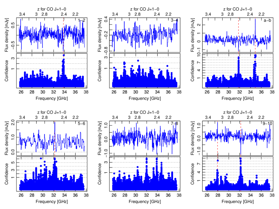
Figure 1.— The first twelve sets of spectra and detection confidence plots for targets labeled by target number in Table 1 and described in Section 3. The upper panel in each set is the difference spectrum for each pair (panel letter in the upper right hand corner). The lower panel is a detection confidence plot as described in the text. Coherent columns of dots indicate detections that are insensitive to binning parameters. Vertical dashed lines mark detections or tentative detections.

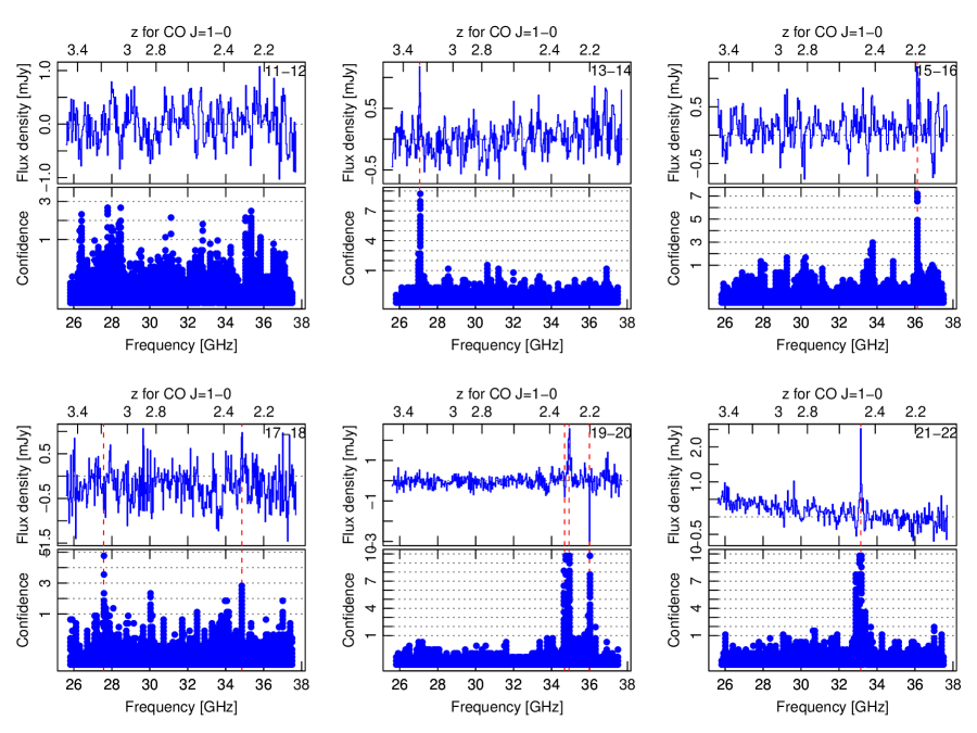
Figure 1 (cont.).— The second twelve sets of spectra and detection confidence plots for targets labeled by target number in Table 1 and described in Section 3.

Our brief comments on individual spectra are:

J083051.0+013224 and J084933.4+021443 (Fig. 1, 1-2): Only the second target in the pair (emission appears in the negative sense) is detected. D.A. Riechers (priv. comm. 2011) has detected a single strong line with the CARMA observatory toward the first in the pair. If the line were CO $J=3-2$, J083051.0+013224 would lie at a redshift with the $1-0$ line in a low-noise region of the Zpectrometer band. This is a statistically significant nondetection that we discuss in section 3.1.

J083929.5+023536 and J084259.9+024958 (Fig. 1, 3-4): Neither target is clearly detected in this spectrum.

J090302.9$-$014127 and J091305.0$-$005343 (Fig. 1, a-c): Clear detections of both targets. The high confidence at slightly lower frequency than the strong positive line is likely an artifact, as even a modest dip can be far from the local amplitude mean, a signature the detection algorithm interprets as a line.

J091840.8+023047 and J085111.7+004933 (Fig. 1, 5-6): Clear detection of the first target in the pair. The continuum offset from zero shows that the first target has a higher continuum flux than the second target.

J091948.8$-$005036 and J092135.6+000131 (Fig. 1, 7-8): Neither target is clearly detected in this spectrum. Residual large-scale structure may obscure what could be tentative detections. Even small noise fluctuations at the tops of large-scale positive and negative structures are far from local means, so they register strongly in the confidence plot.

J113526.3$-$014605 and J113243.1$-$005108 (Fig. 1, 9-10): Clear detections of both targets. Some spurious high confidence peaks are associated with each of the bright lines.

J113833.3+004909 and J113803.5$-$011735 (Fig. 1, 11-12): Neither target is clearly detected in this spectrum.

J114637.9$-$001132 and J115112.3$-$012638 (Fig. 1, 13-14): Clear detection of the first target.

J115820.2$-$013753 and J114752.7$-$005832 (Fig. 1, 15-16): Clear detection of the first target.

J132426.9+284452 and J133008.3+245860 (Fig. 1, 17-18): Tentative detection of the first target. Baseline structure to slightly higher frequencies makes it difficult to find a local baseline, so the line parameters are uncertain.

J134429.4+303036 and J133649.9+291801 (Fig. 1, 19-20): Clear detections of both targets, with one line in the positive sense and two in the negative sense. We attribute the stronger negative line with the SPIRE source. For completeness, we assign the other negative line a tentative formal detection because it is uncharacteristically broad for a spurious signal, but it is close to the positive-sense line where the local mean changes rapidly and may throw off the detection algorithm.

J141351.9$-$000026 and J142751.0+004233 (Fig. 1, 21-22): A strong detection of the first target. The high confidence measures for dips to either side are most likely due to a high local mean in the region. The dips are rather wide to be due to a galaxy, so it is unlikely that they represent detections. The continuum slope indicates a difference in spectral index between the two targets.

Overall, we detected 11 of the 24 targets in our sample. Two of the detections were blind independent confirmations of sources with established redshifts ID.17b in Lupu et al., 2010 and ID.130 in Frayer et al., 2011. This success rate is similar to that of detections from the Plateau de Bure millimeter-wave interferometer starting from optical redshift catalogs (e.g., Neri et al., 2003; Greve et al., 2005; Tacconi et al., 2006; Bothwell et al., 2012), but without the complications associated with finding optical redshifts for submillimeter sources (see, e.g., Chapman et al., 2005). Section 3.1 contains a more extensive discussion of detection completeness. In addition to the 11 detections, we also list two tentative detections, denoted by italics in Table 3 and (for J132426.9+284452) with open circles in the figures. Line parameters for tentative detections were too uncertain for robust error estimates.

Based on the submillimeter photometric selection and line strength, we initially derived redshifts assuming that the lines were the redshifted CO $J=1-0$ transition rather than CO $J=2-1$ from a $5.1\leq z\leq 8.0$ galaxy or a line from a species other than CO. This assumption has proved correct for all 11 sources, which have other observed lines, most starting with redshifts from the Zpectrometer observations (D.A. Riechers, priv. comm. 2011; P.P. van der Werf, priv. comm. 2011; Lupu et al., 2010).

Table 3 summarizes observed and derived source parameters. For detected lines, the parameters are from single-component fits to Gaussian lineshapes, with errors given by the statistical uncertainties in the fit at the 68% (“$1\sigma$”) confidence level. Gaussian fits to the convolutions of Gaussian line shapes and the correlator’s sinc instrumental profile shows that linewidth corrections are unimportant for linewidths above 200 km s^-1 FWHM (the correction is 12% when the Gaussian line and sinc FWHMs are equal, falling below 1% when the Gaussian’s FWHM is 1.5 times the sinc’s FWHM or wider). All lines are broader than this, so we make no corrections. The table also contains estimates of the total infrared (8–1000 $\mu$m) fluxes and dust temperatures obtained from fits to the SPIRE photometry (H-ATLAS collaboration, priv. comm. 2010), as discussed later. In addition to the detections from this program, Table 3 also includes CO $1-0$ data from a previous Zpectrometer detection of H-ATLAS J090311.6+003906 (Frayer et al., 2011, ID.81).

3.1. Flux relationships and detection completeness

We have firm detections of 11 of the 24 targets in our program, a number large enough to draw some sample conclusions. Here we use the molecular and continuum flux information to explore the detection completeness and to evaluate possible reasons for CO nondetections. Figure 2 explores the relationship between 350 $\mu$m flux density, $S_{\nu}(350)$, and the CO $J=1-0$ integrated flux, $S_{\nu}({\rm CO})\Delta{v}$. Sources without CO detections have zero amplitude in this plot, and the open circle denotes a tentative CO detection. Line nondetections generally fall to lower 350 $\mu$m flux densities, but several galaxies are bright in continuum but not detected in CO. We can take the third-brightest $S_{\nu}(350)$ source in our sample (J083051.0+013224, target number 1 in figures and tables) as an example of a nondetection that implies a galaxy with a redshift outside the Zpectrometer band or an abnormally low CO to continuum flux ratio. The former seems more likely in this case: as noted above, CARMA has a clear detection of a mid-$J$ CO line from this source, but deep integrations by the Zpectrometer and other instruments have not found other lines corresponding to a redshift within the Zpectrometer’s $z=2$–3.5 band.

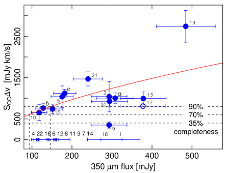
Figure 2.— Integrated CO flux $S_{\nu}({\rm CO})\Delta{v}$ versus 350 $\mu$m flux density $S_{\nu}(350)$ for CO-detected and CO-undetected sources from our sample. CO nondetections have been assigned zero flux. Horizontal dashed lines show completeness levels for line detections derived from our 400 km s^-1 linewidth simulations, with corresponding $S_{\nu}(350)$ derived from the power-law fit shown by the smooth curve. All galaxies with CO nondetections have 350 $\mu$m flux densities above the 70% completeness limit for detections if a simple CO-continuum flux scaling law holds (see text). This implies that chance alone cannot explain the fraction of galaxies in the sample that we do not detect, but that some galaxies have redshifts outside the Zpectrometer band or contain relatively little molecular gas. Points are labeled by target numbers given in the tables.

Most likely, some fraction of the nondetected galaxies have redshifts that are not well predicted by continuum properties, while others have CO $1-0$ lines that are fainter than our detection threshold. Before we simply ascribed CO nondetections to galaxies with observed luminosities below some threshold, we first examined the line detection completeness and the relationship between line and continuum fluxes. Estimating line detection completeness in broadband spectra is complicated by system temperature and nonideal noise that vary with frequency; this frustrates any attempt to define a quantity such as the baseline rms in narrowband spectra that could specify a simple detection limit. We estimated completeness levels for nondetections by simulation, adding sets of synthetic lines as frequency combs across subscans for all sources, running the modified spectra through the data reduction pipeline, and inspecting the spectra to see which synthetic lines we could clearly identify. With a comb of seven 400 km s^-1 wide lines (a width close to the median of the astronomical source linewidths) across each spectrum, we recovered 90% of the synthetic lines with CO integrated intensity $S_{\nu}({\rm CO})\Delta{v}$ = 800 mJy km s^-1, 70% of the lines with $S_{\nu}({\rm CO})\Delta{v}$ = 600 mJy km s^-1, and 35% of those with $S_{\nu}({\rm CO})\Delta{v}$ = 400 mJy km s^-1. Taking $S_{\nu}({\rm CO})\Delta{v}$ = 600 mJy km s^-1as the typical lower limit for our detections, the simulation gives 70% completeness for 400 km s^-1 lines, 90% completeness for 200 km s^-1 lines, and 40% completeness for 800 km s^-1 lines. This shows that the statistical algorithm is most sensitive to peak intensity for lines near detection thresholds. The average completeness for these three widths is 67%, so 70% is representative for a set of lines with various widths and 600 mJy km s^-1.

A somewhat monotonic relationship between the continuum and line fluxes in DSFGs must exist: energy balance requires that galaxies with little far-IR continuum luminosity will have weak molecular emission. The exact relationship is unknown, but a power-law fit established a representative correspondence between $S_{\nu}({\rm CO})\Delta{v}$ and 350 $\mu$m flux densities $S_{\nu}(350)$ for sources with CO detections. This fit yielded equivalent limits of $S_{\nu}(350)$ = 150 mJy, 90 mJy, and 50 mJy for 90, 70, and 35% completeness for the median (400 km s^-1) linewidth, as shown in Figure 2. Given the $S_{\nu}({\rm CO})\Delta{v}$–$S_{\nu}(350)$ distribution, the exact form of the continuum–line relationship is unimportant over the relatively small range at low flux densities, and a linear fit gave essentially the same values. Excluding the extreme high-flux point from the fit flattens the $S_{\nu}({\rm CO})\Delta{v}$–$S_{\nu}(350)$ relationship, pushing the completeness limits to lower continuum flux densities. Pushing the completeness limits to higher flux densities would require a steeper relationship than could be supported by these data with a simple model.

Whatever the exact form of the correspondence between $S_{\nu}({\rm CO})\Delta{v}$ and $S_{\nu}(350)$, all of our targets have $S_{\nu}(350)$ falling above the 70% completeness level (probability of detection) if their CO $J=1-0$ emission falls within the Zpectrometer frequency range. We estimated the number of targets we might expect to have missed due to faint CO flux alone by considering the targets below $S_{\nu}(350)$ = 150 mJy, the approximate 90% completeness level. There are 10 sources in our target list below this limit, of which we detect only two. If chance alone dominates, the detection rate will be given by the binomial distribution. Taking a lower limit of a 70% detection probability, the distribution finds 7 detections as most likely, with $7\pm 3$ detections accounting for 99% of the total probability. The probability of detecting just two sources is 0.1%. Increasing either the detection probability or the flux limit corresponding to a given detection probability reduces the probability of detecting just two of ten sources.

If chance alone ruled, we should therefore have detected some 2 to 5 more weak sources. Considering the additional four nondetections with 350 $\mu$m flux densities significantly above the nominal 90% completeness limit, this analysis points to a strong disparity between actual and expected detections. We conclude that chance is not the only reason for nondetections, but that systematic effects are also important: some of the sources could not be detected because their redshifts are outside of the Zpectrometer’s band, some because they have lower $S_{\nu}({\rm CO})\Delta{v}$/$S_{\nu}(350)$ ratios than the detected sources, some because their lines are weak and broad (although there is no sign of these even though the eye is good at picking out correlated channels), or some combination.

3.2. Redshift distribution

Zpectrometer redshifts for the H-ATLAS sources provide an independent sample for comparison with previous spectroscopic redshift surveys. Comparing surveys, we find that the redshift distributions of the “350 $\mu$m peaker” galaxies with Zpectrometer detections and those of the radio-preselected SMGs (Chapman et al., 2005) that fall within the Zpectrometer’s redshift range are strikingly similar, although the source selection and lines used in the redshift measurements were quite different: our galaxies are 350 $\mu$m-bright targets from a wide-area survey that highlights lensed sources, while the Chapman et al. (2005) galaxies must be bright at 850 $\mu$m and 20 cm radio continuum. Figure 3a gives the binned distribution for the galaxies with Zpectrometer CO detections. The median of the Zpectrometer CO redshifts is $z=2.47\pm 0.11$, and the mean is $z=2.60\pm 0.10$ (68% confidence levels by bootstrap analysis), both well below the band center at $z=2.78$. Figure 3a shows that the peak of the observed density function is near $z\sim 2.3$, agreeing well with the peaks found for optical spectroscopic redshifts of SCUBA-selected sources (Chapman et al., 2005), and for photometric redshifts of both Herschel-selected sources bright at 350 $\mu$m (Amblard et al., 2010) and 870 $\mu$m-selected sources identified by LABOCA (Wardlow et al., 2011).

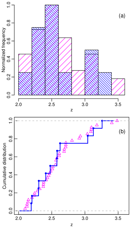
Figure 3.— Comparisons of the redshift distribution of galaxies from our Zpectrometer CO survey and those from the Chapman et al. (2005) optically-derived redshift survey of SMGs that fall within the Zpectrometer’s redshift range. Panel (a) is the binned distribution with Zpectrometer data in close hatch and Chapman et al. (2005) data in coarser hatch. Panel (b) gives the cumulative distribution functions, which do not rely on bin width choices; Zpectrometer data are solid points connected by lines, Chapman et al. (2005) data open triangles. The two distributions are strikingly similar (a Kolmogorov-Smirnov test returns a probability of 0.995 that they are drawn from the same parent population) although the selection criteria are completely different. This suggests a common parent population (and perhaps selection effects) for the SPIRE- and 870 $\mu$m-selected galaxies.

Figure 3b gives the cumulative distribution functions of the Zpectrometer and the Chapman et al. (2005) sample redshifts, allowing a clean comparison free of binning effects. It shows that the distributions are indistinguishable; a Kolmogorov-Smirnov test gives a probability of 0.995 that the two underlying distributions are the same. Such good agreement must in part reflect random chance in a statistically small sample, but nevertheless it is clear that the two distributions are very similar. There is otherwise no a priori reason that the distributions should be so similar: for instance, the Chapman et al. (2005) sample could be concentrated to lower redshifts because of the radio pre-selection, while the Zpectrometer detections could highlight a population of galaxies with strong molecular but very little rest-frame UV line emission.

Another similarity between the Zpectrometer sample and galaxies detected in millimeter-wave CO followup from optical redshift catalogs is the distribution of CO linewidths. Linewidths trace the dynamics, and thus to some extent masses, of the galaxies, and are not strongly affected by lensing. Full width at half maximum (FWHM) linewidths in the Zpectrometer sample range from 210 to 1180 km s^-1, with a median width of $400\pm 100$ km s^-1 (68% confidence levels by bootstrap analysis). In general this is somewhat narrower than the widths of mid-$J$ lines in the millimeter-wave studies of Greve et al. (2005) and Tacconi et al. (2006), but a permutation test shows that the difference in median widths between the studies is significant at only the 70% level, and could easily be from small number statistics. Combining the samples, a characteristic width of about 500 km s^-1 is representative for DSFGs. In absolute terms, the widest $1-0$ lines are very broad, however, including two with FWHM linewidths greater than 1100 km s^-1. If tracing virialized matter, these widths correspond to emission from very massive galaxies or interacting massive galaxies.

3.3. Continuum properties

Spectroscopic redshift measurements unambiguously break the $T_{D}$-$z$ degeneracy (e.g., Blain, 1999) that renders dust temperature estimates uncertain for galaxies without firm redshift measurements. We fit a simple optically thin single-temperature dust model with dust emissivity $\beta=1.5$ to the 250, 350, and 500 $\mu$m SPIRE flux densities. To estimate the observed total infrared (rest-frame 8–1000 $\mu$m) luminosity, we joined the far-infrared fit smoothly in slope to a power-law spectrum with form $S_{\nu}\propto\nu^{-1.4}$ at short wavelengths (Blain et al., 2003). Assuming that the same gravitational magnification $\mu$ applies to emission in all far-IR wavebands, lensing should not affect temperature estimates, but it will scale the intrinsic luminosity $L_{\rm IR}$ so the observed infrared luminosity is $\mu L_{\rm IR}$.

Table 3 contains the model results and Monte-Carlo error estimates for individual galaxies. Excluding the two $z>3.1$ galaxies, the dust temperature is $34\pm 2$ K averaged over all of the detected sources, with a slight dependence on the observed 350 $\mu$m flux density (Fig. 4b) or, equivalently, $\mu L_{\rm IR}$. Little temperature scatter is to be expected among the detected galaxies because the source selection criteria favored similar SPIRE-band SEDs. Temperatures near 35 K are similar to those derived from other surveys of SMGs $35\pm 3$ K, Kovács et al., 2006; $34\pm 5$ K, Chapman et al., 2010; $37\pm 1$ K, Wardlow et al., 2011. The two highest-$z$ galaxies in our sample have temperatures of about 40 K, a temperature higher than scatter alone can explain. Varying the dust emissivity parameter $\beta$ from 1.2 to 1.7 did not change the dust temperatures by more than 3 K. Dust emission models that allow for dust emission optical depths yield temperatures about 15 K higher than those from the optically thin model; we quote the optically thin results to facilitate comparisons with previous work, most of which uses the same formalism.

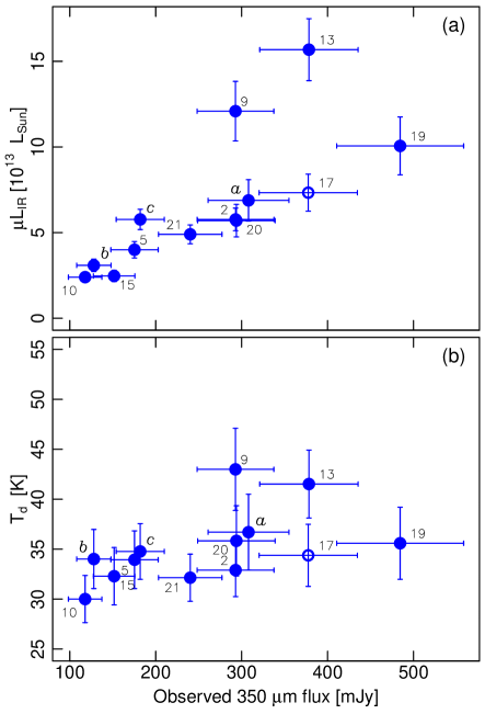
Figure 4.— Panel (a) gives the observed IR luminosity versus observed 350 $\mu$m flux density $S_{\nu}(350)$, showing that the luminosity scales reasonably well with flux density, even in the presence of a range of redshifts and dust temperatures. Panel (b) shows that the derived characteristic dust temperatures are nearly constant with $S_{\nu}(350)$, possibly at least in part from selection effects. The highest two points in both panels are from the two galaxies in our sample with $z\gtrsim 3.1$. Points are labeled by target numbers given in the tables.

Figure 4a shows that the 350 $\mu$m flux density is an excellent proxy for the observed infrared luminosity $\mu L_{\rm IR}$ at $z\sim 2$–3. The two points falling above the general trend are the two galaxies with the highest redshifts, $z>3.1$, in our sample. Excluding these two galaxies, we derive $\mu L_{\rm IR}=(S_{\nu}(350\,\mu{\rm m})/(51\,\rm{mJy})+0.4)\times 10^{13}\,L_{\odot}$. Apart from the two galaxies at $z>3.1$ there is no dependence of $\mu L_{\rm IR}$ on redshift within errors.

3.4. Comparison of photometric and line redshifts

One of the goals of this project was to provide a data set suitable for evaluating the precision of photometric redshifts against spectroscopic measurements. Here we make a first-cut comparison of techniques based on simple SPIRE 3-band colors and on fitting to template galaxy SEDs.

With galaxies chosen as “350 $\mu$m peakers,” the simplest color selection is a flux ratio that estimates the SED’s peak wavelength. Since the 250 $\mu$m and 500 $\mu$m bands straddle the emission peak their ratio provides this estimate, reflecting some combination of temperature and redshift. As section 3.3 shows, our sample of galaxies has a small range of dust temperatures, so we can test whether there is a simple relationship between the observed SED peak wavelength and redshift. Figure 5 shows that there is a relationship between the peak wavelength, as given by the 250 $\mu$m/500 $\mu$m flux density ratio, and spectroscopic redshift for galaxies with CO detections. For these galaxies the 250 $\mu$m/500 $\mu$m flux density ratio predicts redshifts within $\Delta z=0.3$ (standard deviation of the redshift error). Other combinations of continuum flux densities and ratios are less successful at predicting redshifts than the peak wavelength. For example, both the CO-detected and nondetected target galaxies fall along a common locus in a 500 $\mu$m/350 $\mu$m–350 $\mu$m/250 $\mu$m color-color diagram, but the galaxies are well mixed in redshift along that locus.

A more general method of estimating redshifts is to take SEDs of galaxies with known redshift and temperature as templates, then find which redshifted template best matches the observed SED. Template fits are not very tightly constrained by SPIRE data alone because the 250, 350, and 500 $\mu$m bands lie near the peak of the observed-frame SED, however. Flux ratios near the peak have little dynamic range and consequently cannot provide strong constraints: the maximum $S_{\nu}(350)/S_{\nu}(500)$ and $S_{\nu}(350)/S_{\nu}(250)$ ratios are about 1.6.

Figure 6 shows the redshift error $\Delta z$ versus redshift $z$ for the detected galaxies comparing results from the simple $S_{\nu}(250)/S_{\nu}(500)$ ratio and those from independent template fitting codes by co-authors Clements, González-Nuevo, and Wardlow. Each estimates the redshift by minimizing the chi-squared deviation of the data points compared with one or more observed SEDs of galaxies with known redshifts. Minimizing chi-squared by shifting the templates in wavelength gives the redshift, while the widths of the chi-squared values versus shift provide redshift error estimates. Comparing the template fitting with the linear fit between $z$ and $S_{\nu}(250)/S_{\nu}(500)$ shown in Fig. 5, shows that the linear fit gives the lowest dispersion in $\Delta z$ for most of the detected galaxies. Redshifts from an SED corresponding to the Cosmic Eyelash galaxy SMM J2135$-$0102 González-Nuevo et al., 2012, with SED template from Ivison et al., 2010 and Swinbank et al., 2010 are nearly as accurate as those from the linear fit. Comparison with models that choose from libraries of extragalactic SEDs shows these have generally poorer agreement than constrained models for most of the detected galaxies, with $\Delta z\approx 0.5$–1 and internal error estimates smaller than the actual redshift deviation between observation and model. Their errors are lower than those of the $S_{\nu}(250)/S_{\nu}(500)$ ratio or Eyelash fits for the two galaxies at $z>3.1$, however. This result emphasizes the difficulty of fitting curves with only a few samples near the peak; photometric redshifts incorporating substantially longer-wavelength data are substantially more accurate (see, e.g., photometric redshifts including MAMBO 1200 $\mu$m data in Negrello et al., 2010).

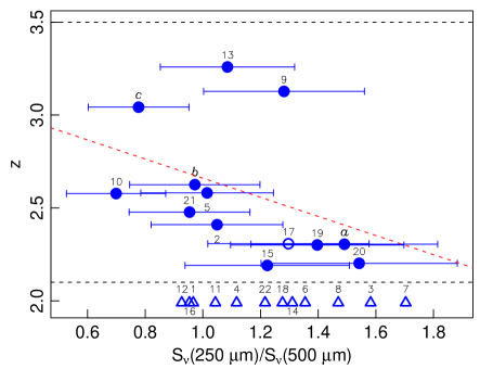
Figure 5.— Galaxy redshift $z$ versus 250 $\mu$m/500 $\mu$m continuum flux density ratio (solid points; open point for a tentative detection). Dashed horizontal lines mark the Zpectrometer’s band edges. CO nondetections (triangles) are plotted outside the band at an arbitrary $z=2$. For galaxies with CO detections, the figure shows that SPIRE colors give $\Delta z\sim 0.3$ for this carefully filtered homogeneous sample. Points are labeled by target numbers given in the tables.

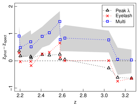
Figure 6.— Photometric redshift errors versus spectroscopic redshift. For the sources with CO $J=1-0$ redshifts, either the linear fit (triangles; Fig. 5) or template fitting against the Eyelash SED (crosses) provides redshift estimates within $\Delta z\approx 0.3$ for $z\leq 3.1$. Dashed lines highlight grouping by method only. Template fits that automatically select from a library of SEDs (squares) generally predict redshift to $\Delta z\approx 0.5$-1; the grey background shows the typical internal uncertainty for the template fits. Models that choose between multiple SEDs predict redshifts outside the Zpectrometer band for several of the nondetected sources, even though the linear and Eyelash templates place them within the band, and have lower errors for the $z>3$ sources. As discussed in the text, this indicates that selection effects are important in the agreement between Eyelash SED and CO detections.

We emphasize that the correspondence between CO $J=1-0$ detections and SPIRE 250 $\mu$m/500 $\mu$m color or Eyelash template redshifts yields no redshift information about the galaxies that we do not detect in the CO $J=1-0$ line. Galaxies with and without detections span nearly the same 250 $\mu$m/500 $\mu$m flux density ratios (Fig. 5), and the success of the Eyelash template may simply arise from its ability to identify the $T\sim 35$ K galaxies we find in CO. As we discussed in section 3.1, some fraction of galaxies with continuum properties similar to galaxies with CO detections very likely fall outside the Zpectrometer’s band.

3.5. Lens magnifications

Lens magnifications ($\mu$) are needed to convert the observed fluxes to intrinsic luminosities. Determining magnification is generally done by constraining a model of the source-lens pair with an image of the gravitationally-distorted source galaxy. Detailed lens models are not yet available for most of our sources. We do have velocity-resolved spectra, however, and can take an alternative approach of comparing observed and intrinsic luminosities established by an empirical luminosity-linewidth relationship similar in spirit to the Tully-Fisher relation (Tully & Fisher, 1977). Without correction for galaxy inclination or dispersion in intrinsic galaxy properties, such a relationship cannot be exact, but it can provide approximate estimates of lensing magnifications.

Since the galaxies with Zpectrometer CO detections seem to be quite typical of the general SMG population, as we discussed above, we assume that only lens magnifications modify the observed typical luminosity distributions of galaxies detected in CO $J=1-0$. Following the method of Bothwell et al. (2012), as outlined below, we find an empirical intrinsic integrated line luminosity-linewidth relationship $L^{\prime}=a\left(\Delta v_{\rm FWHM}\right)^{b}$ from galaxies with published CO $J=1-0$ intensities, widths, and magnifications. This relationship forms the basis to solve for the unknown magnification $\mu$ that scales the true line luminosity $L^{\prime}$ to an apparent luminosity $L^{\prime}_{\rm apparent}=\mu L^{\prime}$, or

$$\mu=\frac{L^{\prime}_{\rm apparent}}{L^{\prime}}=\frac{L^{\prime}_{\rm apparent}}{a\left(\Delta v_{\rm FWHM}\right)^{b}}\;.$$ (1)

Figure 7 shows $L^{\prime}_{{\rm CO}J=1-0}$ for 15 $z=2$–4 SMGs from the literature versus linewidth, with corrections for lens magnification when needed CO data from Harris et al., 2010; Carilli et al., 2010; Ivison et al., 2011; Riechers et al., 2011a; magnifications as needed from Smail et al., 2002. Points for these galaxies fall close to a power law fit with relatively small scatter. Inserting the fit parameters into equation (1), we obtain

$$\mu=3.5\,\frac{L^{\prime}_{\rm apparent}}{10^{11}\,{\rm K\,km\,s}^{-1}{\rm\,pc}^{2}}\left(\frac{400\,{\rm km\,s}^{-1}}{\Delta v_{\rm FWHM}}\right)^{1.7}\;,$$ (2)

with the units for line luminosity $L^{\prime}$ as defined in Solomon et al. (1992). Apparent line luminosities for the H-ATLAS galaxies with Zpectrometer CO measurements, uncorrected for lens magnification, are also plotted in Figure 7 . As expected for a flux-limited sample, these galaxies have a narrower range of luminosities than the comparison sample from the literature. Galaxies with narrower linewidths, which will generally have lower luminosities, require more magnification to reach the observational detection threshold.

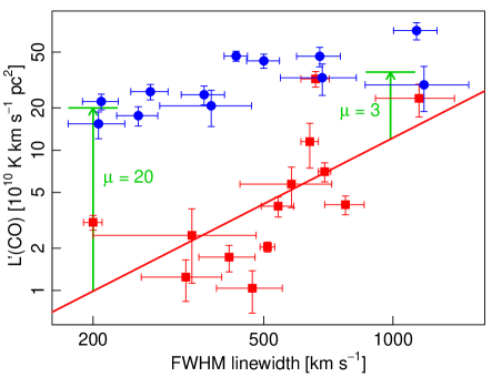
Figure 7.— Square points indicate line luminosities $L^{\prime}_{\rm CO}$ versus CO $J=1-0$ FWHM linewidths for 15 sources with redshifts, fluxes, and magnifications as needed from the literature CO data from Harris et al., 2010; Carilli et al., 2010; Ivison et al., 2011; Riechers et al., 2011a; magnifications as needed from Smail et al., 2002. The solid line shows a power-law fit to these data, representing an estimate of the intrinsic line luminosity versus linewidth for typical galaxies. Round points show the observed line luminosities versus widths for the Zpectrometer sample (values from Table 3), without correction for lens magnifications. The literature sample has a steep power-law relation with modest scatter, while the Zpectrometer sample shows a much flatter trend. Intrinsically weaker sources require higher magnification to rise above the observational detection threshold, which is approximately constant in flux. We scaled the observed line luminosity for each of the Zpectrometer sources by the prediction from the power-law estimate of its likely magnification $\mu$, as given in Table 3. This method yielded a range of $\mu\approx 3$–20 and a median of $\mu=10$ for the Zpectrometer sample.

Table 3 lists the lens magnifications derived from equation (2). The empirical magnification distribution is approximately uniform over its range of 3 to 20, with both median and mean equal to 10. Simple uncertainty estimates for the scaling term and power law index are not available because the two are not independent, but a bootstrap analysis provides $\sim$68% confidence bounds on $\mu$ for each galaxy in Table 3. Fractional uncertainties range from about 30% at a minimum near 500 km s^-1, climbing to about 50% at 300 and 1200 km s^-1, and about 100% at 200 km s^-1. The divergence toward low $\Delta v_{\rm FWHM}$ is also a reminder that the (unknown) inclination corrections become large for galaxies with observed low linewidths. It is possible that some of the sources with broad CO lines and low inferred amplifications from equation (2) are intrinsically hyper-luminous systems which are not significantly magnified at all; the magnification uncertainty encompasses that possibility.

Table 3List of galaxies with observed CO line luminosities and estimates for lens magnifications $\mu$ and corrected (intrinsic) dust luminosities and gas masses. The median value of $\mu=10$. Mass calculations are from $M=\alpha\,L^{\prime}$, with $\alpha=0.8$ $M_{\odot}$ (K km s^-1 pc²)^-1 (Downes & Solomon, 1998) to ease comparisons using this value as a standard. Masses from $J=1-0$ intensities are likely to provide larger masses by a factor between 1.5 and 2 compared with those derived from millimeter-wave observations (discussion and references in Harris et al., 2010). Errors do not include uncertainties in $\alpha$ (see, e.g., Tacconi et al., 2008, for a review). For comparison with other work that assumes $\mu\approx 10$, the last two columns contain luminosity and mass estimates with $\mu=10$, with errors incorporating a nominal $\Delta\mu/\mu=0.5$.

H-ATLAS Name	$L^{\prime}_{\rm obs,CO}\,[10^{10}$ K	$\mu$	$L_{IR}/\mu$	$M_{\rm gas}/\mu$	$L_{IR}/10$	$M_{\rm gas}/10$	Target
	km s-1 pc${}^{2}]$		$[10^{12}\;L_{\odot}$]	$[10^{10}\;M_{\odot}$]	$[10^{12}\;L_{\odot}$]	$[10^{10}\;M_{\odot}$]	No.
J084933.4+021443	$29.2\pm 10.4$	$2\pm 1$	$28.8\pm 19.6$	$11.7\pm 8.0$	$5.8\pm 3.5$	$2.3\pm 1.4$	$2$
J090302.9$-$014127	$26.1\pm 3.3$	$18\pm 8$	$3.8\pm 1.9$	$1.2\pm 0.6$	$6.9\pm 3.5$	$2.1\pm 1.1$	$a$
J090311.6+003906	$46.9\pm 3.8$	$14\pm 4$	$4.1\pm 1.2$	$2.7\pm 0.8$	$5.8\pm 2.9$	$3.8\pm 1.9$	$c$
J091305.0$-$005343	$24.9\pm 3.8$	$10\pm 4$	$3.1\pm 1.2$	$2.0\pm 0.8$	$3.1\pm 1.6$	$2.0\pm 1.0$	$b$
J091840.8+023047	$32.9\pm 8.3$	$5\pm 1$	$8.0\pm 2.9$	$5.3\pm 1.9$	$4.0\pm 2.2$	$2.6\pm 1.5$	$5$
J113243.1$-$005108	$20.7\pm 6.0$	$8\pm 3$	$3.0\pm 1.3$	$2.1\pm 0.9$	$2.4\pm 1.4$	$1.7\pm 1.0$	$10$
J113526.3$-$014605	$15.4\pm 3.3$	$17\pm 11$	$7.1\pm 4.8$	$0.7\pm 0.5$	$12.1\pm 6.6$	$1.2\pm 0.7$	$9$
J114637.9$-$001132	$46.7\pm 7.4$	$7\pm 2$	$22.4\pm 6.9$	$5.3\pm 1.6$	$15.7\pm 8.2$	$3.7\pm 2.0$	$13$
J115820.2$-$013753	$17.6\pm 2.8$	$13\pm 7$	$1.9\pm 1.0$	$1.1\pm 0.6$	$2.5\pm 1.3$	$1.4\pm 0.7$	$15$
J133649.9+291801	$22.2\pm 2.9$	$23\pm 15$	$2.5\pm 1.6$	$0.8\pm 0.5$	$5.7\pm 2.9$	$1.8\pm 0.9$	$20$
J134429.4+303036	$71.2\pm 10.0$	$4\pm 2$	$25.2\pm 14.2$	$14.2\pm 8.0$	$10.1\pm 5.2$	$5.7\pm 3.0$	$19$
J141351.9$-$000026	$43.4\pm 5.0$	$10\pm 3$	$4.9\pm 1.3$	$3.5\pm 0.9$	$4.9\pm 2.5$	$3.5\pm 1.8$	$21$

Magnifications from the luminosity-linewidth relation (2) compare well with values from the two galaxies in the H-ATLAS survey that have both Zpectrometer detections and preliminary lens models from image reconstruction with lens and source galaxies at known redshifts. For J090311.6+003906 (ID.81; CO data from Frayer et al., 2011), the CO linewidth-luminosity relationship in equation (2) predicts $\mu=14\pm 4$, while Negrello et al. (2010) quote $\mu\sim 19$ (range 18–31) from their modeling. For J091305.0$-$005343 (ID.130), equation (2) predicts $\mu=10\pm 4$ while Negrello et al. (2010) quote $\mu\sim 6$ (range 5–7).

Table 3 provides estimates of the intrinsic luminosities and gas masses corrected by the source-specific magnification factors, and also by the median $\mu=10$. Most of the galaxies appear to have intrinsic luminosities typical of ULIRGs, although three are candidate hyper-LIRGs, with luminosities greater than $10^{13}\,L_{\odot}$. Gas mass estimates use the same CO luminosity-to-mass conversion factor as in Greve et al. (2005) and Tacconi et al. (2006) for ease of comparison, $\alpha=0.8$ M_⊙ (K  km s^-1 pc²)^-1 (Downes & Solomon, 1998). Although absolute mass estimates carry double uncertainties from both conversion and magnification factors, they are similar to estimates for SMGs selected from 850 $\mu$m observations that use the same conversion factor.

4. Discussion & Conclusions

Demonstrating an ability to rapidly establish spectroscopic redshifts and molecular line parameters for luminous high-redshift galaxies is a major step forward in exploring the properties of DSFGs. In a single observing season we have added a dozen galaxies with CO $J=1-0$ line detections to the pool of sources for study among the bright “350 $\mu$m peakers” from the Herschel-ATLAS survey.

We established accurate redshifts for sufficient galaxies to compare with an independent survey of SMGs with observed optical redshifts. That survey started with submillimeter source continuum detections in $\sim 15$ arcsecond beams at 850 $\mu$m, associated those with 20 cm radio continuum sources to obtain positions to $\sim 1$ arcsecond, and then used optical spectroscopy to determine redshifts (see e.g., Chapman et al., 2005). Subsequent observations with a millimeter-wave interferometer used the optical redshifts as starting points to determine molecular redshifts from the star-forming gas itself (e.g., Neri et al., 2003; Greve et al., 2005; Tacconi et al., 2006), conclusively connecting the 850 $\mu$m sources with massive molecular clouds in the target galaxies in about half of the attempts. The Zpectrometer CO redshifts, in contrast, started with bright 350 $\mu$m sources with submillimeter photometry indicating rough photometric redshifts, but then made a single step from continuum to molecular line observations with this wideband spectrometer. We find nearly identical redshift distributions for the two surveys, indicating that each sample is representative of a general DSFG population. Coupled with mm-wave molecular spectroscopy of many of the brighter 850 $\mu$m sources (e.g., Neri et al., 2003; Greve et al., 2005; Tacconi et al., 2006), the agreement in distributions between independent samples lays to rest some of the concern that SMG redshift distributions from optical spectroscopy may be influenced by misidentifications between the submillimeter sources and counterpart optical galaxies.

Dust temperatures and linewidths of the galaxies with CO 1–0 detections appear to be similar to SMGs. With spectroscopic redshifts, we are able to break the temperature-redshift degeneracy to find a characteristic temperature of 34 K (in an optically thin formalism), similar to those typically reported for SMGs (Kovács et al., 2006; Chapman et al., 2010; Wardlow et al., 2011). Galaxies with redshifts $z>3$ may be somewhat warmer than those at lower redshift. The CO linewidths have very similar distributions for these H-ATLAS CO $J=1-0$ detections and for SMGs observed in mid-$J$ lines. Both of these comparisons add further to an argument that the bulk of samples selected by bright 850 $\mu$m and SPIRE emission draw from the same parent population.

Most, if not all, of the galaxies we observed appear to be gravitationally lensed. We estimate lens magnifications with an empirical CO linewidth-luminosity relationship made possible with velocity-resolved spectroscopy. We verified magnification agreement within factors close to two for two galaxies with published lens modeling. We find magnifications from 3 to 20, a range matching those for lenses with detailed models, $\mu\approx 5$–30 (Swinbank et al., 2010; Negrello et al., 2010; Gavazzi et al., 2011; Lestrade et al., 2011). In the absence of other information, a typical value of $\mu=10$ is likely to be correct within a factor of two for the bright H-ATLAS galaxies.

With even moderately accurate lens magnification estimates, we can make reasonable estimates of intrinsic luminosities and gas masses of the galaxies in our sample (Table 3). Most have luminosities characteristic of ULIRGs, but there are three targets that could be hyper-LIRGs with luminosities $>10^{13}\,L_{\odot}$. The most luminous of these could well be multiple galaxies within the beam, as their linewidths are broad. Even accounting for lensing magnification, however, the bright H-ATLAS galaxies seem to be drawn from the high-luminosity, high-mass end of the DSFG distribution.

The overall agreement in properties between the Zpectrometer and 850–1200 $\mu$m-selected SMG samples indicates that the two populations are drawn from the same distribution. In principle, the additional selection introduced by lens magnification could have emphasized different properties from the SMG population, but it does not appear to have done so. Lensed sources will be valuable in understanding the properties of the underlying DSFG population, including the SMGs: for observations, magnification by even a factor of a few translates to an order of magnitude reduction in integration time. Detailed studies of the galaxies’ interstellar media in multiple molecular and atomic lines becomes feasible in the bright lensed sample (e.g., Danielson et al., 2011), with magnification also increasing spatial resolution in the source plane (e.g., Swinbank et al., 2010).

Overall, the detection fraction of about half of the targets compares well with other programs that observed molecular lines from high redshift galaxies. A conservative extrapolation of a CO-to-continuum intensity relationship indicates that the nondetection rate is substantially higher than expected from chance alone, evidence that some of the simple photometric redshifts are incorrect. Our selection is from SPIRE photometry identification of “350 $\mu$m peakers.” Comparison of the SPIRE data and CO redshifts indicates that the continuum peak wavelength, deduced from the 250 $\mu$m/500 $\mu$m flux density ratio, predicts the redshift of the galaxies from our carefully-selected sample with $\Delta z\sim 0.3$. The SPIRE colors do not necessarily provide accurate estimates for galaxies we do not detect, however. A simple explanation for some of the nondetections is emission from dust warmer than the $\sim 35$ K characteristic for most of the galaxies with CO detections. The redshift-temperature degeneracy for the observed peak emission wavelength, $\lambda_{\rm peak,obs}\propto T/(1+z)$ (e.g., Blain, 1999) causes problems for photometric selection in the SPIRE bands alone: warmer galaxies with redshift above the Zpectrometer’s upper limit will appear in the target list. It is very likely that this is the reason for the nondetection of the target with third-brightest 350 $\mu$m flux density in this study.

Reasons other than warm galaxies or CO intensities that fall below our observational limit can also contribute to nondetections. Emission from multiple galaxies within the beam at one or more wavelengths can contribute flux to distort the apparent SED, leading to erroneous redshifts from single-component models. This is likely to affect weaker sources preferentially, both because smaller absolute amounts of contaminating flux are increasingly important and because the density of contaminating sources increases with decreasing flux. Multiple distinct temperature components within a source, for instance a central AGN-heated dust region surrounded by less excited material, will also distort the SED. Depending upon the temperature structure within the source and the size and position of the source relative to any lens caustic, differential amplification could distort observed SEDs. SEDs in all these cases will be poorly represented by the simple single-component model we have used in target selection, and photometric redshifts based on SPIRE data alone will fail to some extent.

The observed redshift distribution and the dust SED properties hint at some change in DSFG properties near $z\sim 3$. The redshift cumulative distribution functions for both the Zpectrometer and Chapman et al. (2005) samples show a slope break at $z\sim 2.9$ although they are selected in different ways. This indicates that DSFGs become less common, or are selected less efficiently by continuum properties, above that redshift. An increase in the number of warm galaxies with redshift would both explain the tentative trend in temperature we see and explain the lower CO detection rate. Temperature alone may not suffice to explain the break, and explanations involving more complex SEDs with increasing redshift are attractive as well. Wardlow et al. (2011) use extensive optical and infrared photometry on a sample of 74 870 $\mu$m-selected SMGs, also finding a precipitous drop in submillimeter source counts above $z_{\rm phot}\sim 2.8$ in spite of their sensitivity to emission from warm dust. Increased sample sizes are necessary to establish whether there is a real change in DSFG properties near $z\sim 3$ or not.

The CO data presented here are among the earliest spectroscopic explorations of Herschel-selected galaxies. Continuing observations of the CO $J=1-0$ line by the GBT and Jansky-VLA will provide a more diverse sample of galaxies: some from broadened continuum selection criteria, and some with deeper integrations to reach weaker line emission. Wideband spectrometers now coming on line for the 3 mm band at the LMT and IRAM 30 m will also add to the number of galaxies with known molecular redshifts. An expanded sample will strengthen our understanding of the relationship between molecular and continuum emission in DSFGs.

References

- Alexander et al. (2005) Alexander, D. M., Bauer, F. E., Chapman, S. C., Smail, I., Blain, A. W., Brandt, W. N., & Ivison, R. J. 2005, ApJ, 632, 736
- Alexander et al. (2003) Alexander, D. M., et al. 2003, AJ, 125, 383
- Amblard et al. (2010) Amblard, A., et al. 2010, A&A, 518, L9
- Austermann et al. (2010) Austermann, J. E., et al. 2010, MNRAS, 401, 160
- Baker et al. (2007) Baker, A., Stacey, G., Glenn, J., Erickson, N., Harris, A., & Wootten, A. 2007, in Astronomical Society of the Pacific Conference Series, Vol. 375, From Z-Machines to ALMA: (Sub)Millimeter Spectroscopy of Galaxies, ed. A. J. Baker, J. Glenn, A. I. Harris, J. G. Mangum, & M. S. Yun , 3
- Barger et al. (1998) Barger, A. J., Cowie, L. L., Sanders, D. B., Fulton, E., Taniguchi, Y., Sato, Y., Kawara, K., & Okuda, H. 1998, Nature, 394, 248
- Baugh et al. (2005) Baugh, C. M., Lacey, C. G., Frenk, C. S., Granato, G. L., Silva, L., Bressan, A., Benson, A. J., & Cole, S. 2005, MNRAS, 356, 1191
- Blain (1999) Blain, A. W. 1999, MNRAS, 309, 955
- Blain et al. (2003) Blain, A. W., Barnard, V. E., & Chapman, S. C. 2003, MNRAS, 338, 733
- Blain et al. (2004) Blain, A. W., Chapman, S. C., Smail, I., & Ivison, R. 2004, ApJ, 611, 52
- Blain et al. (2002) Blain, A. W., Smail, I., Ivison, R. J., Kneib, J., & Frayer, D. T. 2002, Phys. Rep., 369, 111
- Bothwell et al. (2012) Bothwell, M. S., et al. 2012, in prep.
- Capak et al. (2008) Capak, P., et al. 2008, ApJ, 681, L53
- Capak et al. (2011) Capak, P. L., et al. 2011, Nature, 470, 233
- Carilli et al. (2010) Carilli, C. L., et al. 2010, ApJ, 714, 1407
- Chapman et al. (2003) Chapman, S. C., Blain, A. W., Ivison, R. J., & Smail, I. R. 2003, Nature, 422, 695
- Chapman et al. (2005) Chapman, S. C., Blain, A. W., Smail, I., & Ivison, R. J. 2005, ApJ, 622, 772
- Chapman et al. (2004) Chapman, S. C., Smail, I., Blain, A. W., & Ivison, R. J. 2004, ApJ, 614, 671
- Chapman et al. (2010) Chapman, S. C., et al. 2010, MNRAS, 409, L13
- Conselice et al. (2003) Conselice, C. J., Chapman, S. C., & Windhorst, R. A. 2003, ApJ, 596, L5
- Coppin et al. (2010a) Coppin, K., et al. 2010a, ApJ, 713, 503
- Coppin et al. (2009) Coppin, K. E. K., et al. 2009, MNRAS, 395, 1905
- Coppin et al. (2010b) —. 2010b, MNRAS, 407, L103
- Daddi et al. (2010) Daddi, E., et al. 2010, ApJ, 714, L118
- Danielson et al. (2011) Danielson, A. L. R., et al. 2011, MNRAS, 410, 1687
- Dannerbauer et al. (2004) Dannerbauer, H., Lehnert, M. D., Lutz, D., Tacconi, L., Bertoldi, F., Carilli, C., Genzel, R., & Menten, K. M. 2004, ApJ, 606, 664
- Davé et al. (2010) Davé, R., Finlator, K., Oppenheimer, B. D., Fardal, M., Katz, N., Kereš, D., & Weinberg, D. H. 2010, MNRAS, 404, 1355
- Downes & Solomon (1998) Downes, D., & Solomon, P. M. 1998, ApJ, 507, 615
- Driver et al. (2009) Driver, S. P., et al. 2009, in IAU Symposium, Vol. 254, IAU Symposium, ed. J. Andersen, J. Bland-Hawthorn, & B. Nordström, 469–474
- Eales et al. (2010) Eales, S., et al. 2010, PASP, 122, 499
- Fixsen et al. (1998) Fixsen, D. J., Dwek, E., Mather, J. C., Bennett, C. L., & Shafer, R. A. 1998, ApJ, 508, 123
- Frayer et al. (1999) Frayer, D. T., Ivison, R. J., Scoville, N. Z., Evans, A. S., Yun, M. S., Smail, I., Barger, A. J., Blain, A. W., & Kneib, J.-P. 1999, ApJ, 514, L13
- Frayer et al. (1998) Frayer, D. T., Ivison, R. J., Scoville, N. Z., Yun, M., Evans, A. S., Smail, I., Blain, A. W., & Kneib, J. 1998, ApJ, 506, L7
- Frayer et al. (2011) Frayer, D. T., et al. 2011, ApJ, 726, L22
- Gavazzi et al. (2011) Gavazzi, R., et al. 2011, ApJ, 738, 125
- Genzel et al. (2003) Genzel, R., Baker, A. J., Tacconi, L. J., Lutz, D., Cox, P., Guilloteau, S., & Omont, A. 2003, ApJ, 584, 633
- Genzel et al. (2010) Genzel, R., et al. 2010, MNRAS, 407, 2091
- González-Nuevo et al. (2012) González-Nuevo, J., et al. 2012, ArXiv e-prints, 1202.0402
- Greve et al. (2005) Greve, T. R., et al. 2005, MNRAS, 359, 1165
- Griffin et al. (2010) Griffin, M. J., et al. 2010, A&A, 518, L3
- Hainline et al. (2011) Hainline, L. J., Blain, A. W., Smail, I., Alexander, D. M., Armus, L., Chapman, S. C., & Ivison, R. J. 2011, ArXiv e-prints, astro-ph/1104.4119
- Harris (2005) Harris, A. I. 2005, Rev. Sci. Inst., 76, 4503
- Harris et al. (2010) Harris, A. I., Baker, A. J., Zonak, S. G., Sharon, C. E., Genzel, R., Rauch, K., Watts, G., & Creager, R. 2010, ApJ, 723, 1139
- Harris et al. (2007) Harris et al., A. I. 2007, in Astronomical Society of the Pacific Conference Series, Vol. 375, From Z-Machines to ALMA: (Sub)Millimeter Spectroscopy of Galaxies, ed. A. J. Baker, J. Glenn, A. I. Harris, J. G. Mangum, & M. S. Yun, 82–92
- Hatsukade et al. (2011) Hatsukade, B., et al. 2011, MNRAS, 411, 102
- Houck et al. (2005) Houck, J. R., et al. 2005, ApJ, 622, L105
- Hughes et al. (1998) Hughes, D. H., et al. 1998, Nature, 394, 241
- Ibar et al. (2010) Ibar, E., et al. 2010, MNRAS, 409, 38
- Ivison et al. (2011) Ivison, R. J., Papadopoulos, P. P., Smail, I., Greve, T. R., Thomson, A. P., Xilouris, E. M., & Chapman, S. C. 2011, MNRAS, 412, 1913
- Ivison et al. (2000) Ivison, R. J., Smail, I., Barger, A. J., Kneib, J.-P., Blain, A. W., Owen, F. N., Kerr, T. H., & Cowie, L. L. 2000, MNRAS, 315, 209
- Ivison et al. (1998) Ivison, R. J., Smail, I., Le Borgne, J.-F., Blain, A. W., Kneib, J.-P., Bezecourt, J., Kerr, T. H., & Davies, J. K. 1998, MNRAS, 298, 583
- Ivison et al. (2010) Ivison, R. J., Smail, I., Papadopoulos, P. P., Wold, I., Richard, J., Swinbank, A. M., Kneib, J., & Owen, F. N. 2010, MNRAS, 261
- Ivison et al. (2005) Ivison, R. J., et al. 2005, MNRAS, 364, 1025
- Kneib et al. (2005) Kneib, J.-P., Neri, R., Smail, I., Blain, A., Sheth, K., van der Werf, P., & Knudsen, K. K. 2005, A&A, 434, 819
- Knudsen et al. (2008) Knudsen, K. K., van der Werf, P. P., & Kneib, J.-P. 2008, MNRAS, 384, 1611
- Kovács et al. (2006) Kovács, A., Chapman, S. C., Dowell, C. D., Blain, A. W., Ivison, R. J., Smail, I., & Phillips, T. G. 2006, ApJ, 650, 592
- Lestrade et al. (2011) Lestrade, J., Carilli, C. L., Thanjavur, K., Kneib, J. ., Riechers, D. A., Bertoldi, F., Walter, F., & Omont, A. 2011, ApJ, 739, L30
- Lindner et al. (2011) Lindner, R. R., et al. 2011, ApJ, 737, 83
- Lupu et al. (2010) Lupu, R. E., et al. 2010, ArXiv e-prints: astro-ph/1009.5983
- Magdis et al. (2010) Magdis, G. E., et al. 2010, MNRAS, 409, 22
- Marriage et al. (2011) Marriage, T. A., et al. 2011, ApJ, 731, 100
- Marsden et al. (2009) Marsden, G., et al. 2009, ApJ, 707, 1729
- Menéndez-Delmestre et al. (2007) Menéndez-Delmestre, K., et al. 2007, ApJ, 655, L65
- Menéndez-Delmestre et al. (2009) —. 2009, ApJ, 699, 667
- Negrello et al. (2007) Negrello, M., Perrotta, F., González-Nuevo, J., Silva, L., de Zotti, G., Granato, G. L., Baccigalupi, C., & Danese, L. 2007, MNRAS, 377, 1557
- Negrello et al. (2010) Negrello, M., et al. 2010, Science, 330, 800
- Neri et al. (2003) Neri, R., et al. 2003, ApJ, 597, L113
- Pascale et al. (2011) Pascale, E., et al. 2011, MNRAS, 415, 911
- Pilbratt et al. (2010) Pilbratt, G. L., et al. 2010, A&A, 518, L1
- Pope et al. (2008) Pope, A., et al. 2008, ApJ, 675, 1171
- Puget et al. (1996) Puget, J.-L., Abergel, A., Bernard, J.-P., Boulanger, F., Burton, W. B., Desert, F.-X., & Hartmann, D. 1996, A&A, 308, L5
- R Development Core Team (2006) R Development Core Team. 2006, R: A Language and Environment for Statistical Computing, R Foundation for Statistical Computing, Vienna, Austria, http://www.R-project.org
- Riechers et al. (2011a) Riechers, D. A., Hodge, J., Walter, F., Carilli, C. L., & Bertoldi, F. 2011a, ApJ, 739, L31
- Riechers et al. (2010) Riechers, D. A., et al. 2010, ApJ, 720, L131
- Riechers et al. (2011b) —. 2011b, ApJ, 739, L32
- Riechers et al. (2011c) —. 2011c, ApJ, 733, L12
- Rigby et al. (2011) Rigby, E. E., et al. 2011, MNRAS, 955
- Scott et al. (2011) Scott, K. S., et al. 2011, ApJ, 733, 29
- Smail et al. (2004) Smail, I., Chapman, S. C., Blain, A. W., & Ivison, R. J. 2004, ApJ, 616, 71
- Smail et al. (1997) Smail, I., Ivison, R. J., & Blain, A. W. 1997, ApJ, 490, L5
- Smail et al. (2002) Smail, I., Ivison, R. J., Blain, A. W., & Kneib, J.-P. 2002, MNRAS, 331, 495
- Smith et al. (2011) Smith, D. J. B., et al. 2011, MNRAS, 416, 857
- Solomon et al. (1992) Solomon, P. M., Downes, D., & Radford, S. J. E. 1992, ApJ, 398, L29
- Somerville et al. (2011) Somerville, R. S., Gilmore, R. C., Primack, J. R., & Dominguez, A. 2011, ArXiv e-prints, astro-ph/1104.0669
- Spergel et al. (2007) Spergel, D. N., et al. 2007, ApJS, 170, 377
- Swinbank et al. (2008) Swinbank, A. M., et al. 2008, MNRAS, 391, 420
- Swinbank et al. (2010) —. 2010, Nature, 464, 733
- Symeonidis et al. (2011) Symeonidis, M., Page, M. J., & Seymour, N. 2011, MNRAS, 411, 983
- Tacconi et al. (2006) Tacconi, L. J., et al. 2006, ApJ, 640, 228
- Tacconi et al. (2008) —. 2008, ApJ, 680, 246
- The Astronomical Almanac (2011) The Astronomical Almanac. 2011, U.S. Naval Observatory and Rutherford Appleton Laboratory
- Tully & Fisher (1977) Tully, R. B., & Fisher, J. R. 1977, A&A, 54, 661
- Valiante et al. (2007) Valiante, E., Lutz, D., Sturm, E., Genzel, R., Tacconi, L. J., Lehnert, M. D., & Baker, A. J. 2007, ApJ, 660, 1060
- Vieira et al. (2010) Vieira, J. D., et al. 2010, ApJ, 719, 763
- Wardlow et al. (2011) Wardlow, J. L., et al. 2011, MNRAS, 414, 917
- Weedman et al. (2006) Weedman, D., et al. 2006, ApJ, 653, 101
- Weiß et al. (2009) Weiß, A., Ivison, R. J., Downes, D., Walter, F., Cirasuolo, M., & Menten, K. M. 2009, ApJ, 705, L45
- Yan et al. (2007) Yan, L., et al. 2007, ApJ, 658, 778