Dynamic Planar Point Location
with Sub-Logarithmic Local Updates

Abstract

We study planar point location in a collection of disjoint fat regions, and investigate the complexity of local updates: replacing any region by a different region that is “similar” to the original region. (i.e., the size differs by at most a constant factor, and distance between the two regions is a constant times that size). We show that it is possible to create a linear size data structure that allows for insertions, deletions, and queries in logarithmic time, and allows for local updates in sub-logarithmic time on a pointer machine. We begin by describing a solution for the $\color[rgb]{0.75,0.30,0.15}1$-dimensional version of the problem, where we can achieve constant time local updates. Then we show how the ideas can be extended to $\color[rgb]{0.75,0.30,0.15}2$ dimensions.

We show that given constant similarity and fatness parameters:

• A set of $\color[rgb]{0.75,0.30,0.15}n$ disjoint intervals in $\color[rgb]{0.75,0.30,0.15}\mathbb{R}^{1}$ can be maintained in an $\color[rgb]{0.75,0.30,0.15}O(n)$ size data structure that supports $\color[rgb]{0.75,0.30,0.15}O(\log n)$ worst-case time insertion, deletion, and point location queries, and $\color[rgb]{0.75,0.30,0.15}O(1)$ worst-case time local updates (Section 3). The data structure can be implemented on a real-valued pointer-machine.

• A set of $\color[rgb]{0.75,0.30,0.15}n$ disjoint fat regions in $\color[rgb]{0.75,0.30,0.15}\mathbb{R}^{2}$ can be maintained in an $\color[rgb]{0.75,0.30,0.15}O(n)$ size data structure that supports $\color[rgb]{0.75,0.30,0.15}O(\log n)$ worst-case time insertion, deletion and point location queries, and $\color[rgb]{0.75,0.30,0.15}O(\log\log n)$ worst-case time local updates (Section 4). The data structure can be implemented on a real-valued pointer-machine.

• We also give bounds that can handle arbitrary similarity and fatness parameters in Theorem 3.3 and Theorem 4.12 for the $\color[rgb]{0.75,0.30,0.15}\mathbb{R}^{1}$ and $\color[rgb]{0.75,0.30,0.15}\mathbb{R}^{2}$ case respectively.

1 Introduction

Planar point location lies at the heart of many geometric problems, and has been a major research topic in computational geometry for the past 40 years. In the static version of the problem, one aims to store a subdivision of the plane such that given a query point $\color[rgb]{0.75,0.30,0.15}q$ in the plane, the cell of the subdivision containing $\color[rgb]{0.75,0.30,0.15}q$ can be retrieved quickly [25, 26, 46, 47, 62]. In the dynamic version of the problem, one also allows changes to the data set, typically adding or removing line segments to the subdivision [5, 9, 34, 35, 53].

The best known dynamic data structures on a real RAM are due to Cheng and Janardan [18], who achieve $\color[rgb]{0.75,0.30,0.15}O(\log^{2}n)$ queries and $\color[rgb]{0.75,0.30,0.15}O(\log n)$ updates where $\color[rgb]{0.75,0.30,0.15}n$ is the size of the subdivision, and Arge et al. [5], who achieve $\color[rgb]{0.75,0.30,0.15}O(\log n)$ queries, $\color[rgb]{0.75,0.30,0.15}O(\log^{1+\varepsilon}n)$ insertions, and $\color[rgb]{0.75,0.30,0.15}O(\log^{2+\varepsilon}n)$ deletions. A central open problem in this area is whether a linear-size data structure exists that can support both queries and updates in logarithmic time, although this is known to be possible in more specific settings such as monotone or rectilinear subdivisions [12, 34, 35]. Husfeldt et al. [41] prove that even in the very strong cell probe model, there are $\color[rgb]{0.75,0.30,0.15}\Omega(\log n/\log\log n)$ lower bounds on both queries and updates.

Despite these theoretical results, practical evidence suggests that updating a data structure should be fast. Intuitively, an update to a data set should not need to depend on $\color[rgb]{0.75,0.30,0.15}n$ at all, unless we need to find the place where the update takes place (i.e., we need to do a point location query). In this paper, we study point location data structures on a collection of fat objects in the plane that support local updates: replace any region by a different region that is similar to the original. We show that the lower bounds on updates can be broken in this setting, while still allowing $\color[rgb]{0.75,0.30,0.15}O(\log n)$ queries and using $\color[rgb]{0.75,0.30,0.15}O(n)$ storage.

The idea of local updates is not new. For example, Nekrich [58] considers (on a word-RAM) the local update operation insert${}_{\Delta}(x,y)$ which inserts a new element $\color[rgb]{0.75,0.30,0.15}x$ into a $\color[rgb]{0.75,0.30,0.15}1$-dimensional sorted list, given a pointer to an existing element $\color[rgb]{0.75,0.30,0.15}y$ that satisfies $\color[rgb]{0.75,0.30,0.15}|x-y|\leq\Delta$ for some distance parameter $\color[rgb]{0.75,0.30,0.15}\Delta$. There is also a related concept called finger updates, where the position of the update is known; see e.g. Fleischer [31]. However, our results are the first in this area that work in a geometric setting, and they can be implemented on a real-valued pointer machine. (See Appendix A for a discussion of computation models.)

In order to obtain our results, we develop several tools which we believe are interesting in their own right, such as a dynamic balanced compressed quadtree with worst-case constant time updates, and a tree decomposition that supports logarithmic searches and constant time local changes (see Section 2.2).

1.1 Problem description

We define the problem in general dimension $\color[rgb]{0.75,0.30,0.15}d$, but restrict our attention to $\color[rgb]{0.75,0.30,0.15}d\in\{1,2\}$ in the remainder of this paper. We use $\color[rgb]{0.75,0.30,0.15}|R|$ to denote the diameter of a region $\color[rgb]{0.75,0.30,0.15}R\subset\mathbb{R}^{d}$, that is, $\color[rgb]{0.75,0.30,0.15}|R|=\max_{p,q\in R}|pq|$. We say two fat regions $\color[rgb]{0.75,0.30,0.15}R_{1},R_{2}\subset\mathbb{R}^{d}$ are $\color[rgb]{0.75,0.30,0.15}\rho$-similar if $\color[rgb]{0.75,0.30,0.15}|R_{1}\cup R_{2}|\leq\rho\min\{|R_{1}|,|R_{2}|\}$, see Figure 1.

Problem 1.1

Given a set $\color[rgb]{0.75,0.30,0.15}\mathcal{R}$ of $\color[rgb]{0.75,0.30,0.15}n$ disjoint fat regions in $\color[rgb]{0.75,0.30,0.15}\mathbb{R}^{d}$, store them in a data structure that allows:

• queries: given a point $\color[rgb]{0.75,0.30,0.15}q\in\mathbb{R}^{d}$, return the region in $\color[rgb]{0.75,0.30,0.15}\mathcal{R}$ that contains $\color[rgb]{0.75,0.30,0.15}q$ (if any) in $\color[rgb]{0.75,0.30,0.15}Q(n)$ time;

• local updates: given a region $\color[rgb]{0.75,0.30,0.15}R\in\mathcal{R}$ and a region $\color[rgb]{0.75,0.30,0.15}R^{\prime}$ that is $\color[rgb]{0.75,0.30,0.15}\rho$-similar to $\color[rgb]{0.75,0.30,0.15}R$, replace $\color[rgb]{0.75,0.30,0.15}R$ by $\color[rgb]{0.75,0.30,0.15}R^{\prime}$ in the data structure in $\color[rgb]{0.75,0.30,0.15}U(n)$ time; and

• global updates: delete an existing region $\color[rgb]{0.75,0.30,0.15}R$ from the data structure or insert a new region $\color[rgb]{0.75,0.30,0.15}R^{\prime}$ into the data structure in $\color[rgb]{0.75,0.30,0.15}Q(n)+U(n)$ time

such that $\color[rgb]{0.75,0.30,0.15}Q(n)=O(\log n)$ but $\color[rgb]{0.75,0.30,0.15}U(n)=o(\log n)$. Note that a local update allows for an arbitrary number of smaller regions to be “between” the old region $\color[rgb]{0.75,0.30,0.15}R$ and the new region $\color[rgb]{0.75,0.30,0.15}R^{\prime}$.

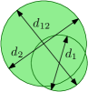
Figure 1: Two $\color[rgb]{0.75,0.30,0.15}\rho$-similar regions for $\color[rgb]{0.75,0.30,0.15}\rho=\frac{d_{12}}{\min\{d_{1},d_{2}\}}$.

1.2 Applications

Tracking moving objects.

A natural application of our data structure is to keep track of moving objects. One may imagine a number of objects of different sizes moving unpredictably in an environment at different speeds. A popular method for dealing with moving objects is to discretize time and process the new locations of the objects at each time step. The naive way to do this is to simply rebuild an entire data structure every time step. Our data structure can be used to process such changes more efficiently.

In computational geometry, there is a large literature on dealing with moving objects (or points). Kinetic data structures are based on the premise that a data structure should not need to be updated each time step, but rather only when some combinatorial feature of a description of objects changes [1, 7, 36, 37]. A fundamental underlying assumption in kinetic data structures is that trajectories of the moving objects are predictable, at least in the short term. However, in many modern real-world scenarios, trajectories are not predetermined, they are discovered in an online and inherently discrete fashion. As a result, several theoretical approaches to deal with unpredictable motion have been suggested recently, in various settings [19, 23, 28, 33, 55, 67]. A common assumption in these works is to bound the maximum displacement after each update (or velocity) of the moving points. An interesting feature of our data structure is that we can simultaneously maintain objects moving at very different scales, with a velocity bound that is dependent on the size of the object.

Data imprecision.

A different motivation for studying this problem comes from the desire to cope with data imprecision. One way to model an imprecise point is to keep track of a region of possible locations of the point [38, 57] (see also [48] and the references therein). Recently, there has been a lot of activity in this area [17, 20, 43, 66]. Although algorithms to deal with imprecise data are beginning to be well understood in a static setting, little effort has been devoted to dealing with dynamic imprecise points. However, in many settings imprecision is inherently dynamic (e.g. time-dependent or “stale” data), or explicitly made dynamic (e.g. updates from new samples of the same point).

One of the simplest geometric queries on a data structure that stores a point set one can imagine is the identity query. Given a query point, is there a point in the data structure that is equal to the query point? When the points in the data structure are imprecise, the answer to this question may have three possible values: “certainly”, “possibly”, or “certainly not.” Distinguishing between the second and last answer comes down to testing whether the query point (which we assume is a precise point) is contained in any of the uncertainty regions of the imprecise points. Therefore, we may view the problem as a dynamic point location problem in a set of changing regions.

If we only wish to support increased precision updates (which would correspond to stationary, but imprecise points), this question is closely related to existing work in the update complexity model [15, 32], in which one attempts to minimize the number (or amount of gained precision) of updates necessary to correctly output some structure; and to work on preprocessing imprecise points [16, 24, 40, 50, 65], in which one tries to prepare a set of imprecise points for faster computation of some structure on the precise points once they become available. While these results do not analyze the time complexity of single updates, they do provide some evidence that sub-logarithmic update time may be possible.

1.3 Solution outline

Geometric data structures are often either based on a recursive decomposition of the data (e.g. a binary search tree) or a recursive decomposition of space (e.g. a quadtree). Neither of those techniques by themselves are strong enough to solve the problem at hand, so our solution combines both techniques. We base our solution on a dynamic balanced compressed quadtree [60], the details of which are covered in Section 2. However, the quadtree is not built on the regions directly. Rather, for each region $\color[rgb]{0.75,0.30,0.15}R\in\cal R$, we store a representative point $\color[rgb]{0.75,0.30,0.15}m$ that lies somehow “in the middle” of $\color[rgb]{0.75,0.30,0.15}R$. We build search structures over the quadtree which allow us to quickly locate the quadtree cells containing relevant data. We answer point-location queries by locating the smallest quadtree cell containing the query point and then searching the quadtree bottom-up for regions which intersect this cell. This approach allows us to handle input described by arbitrary real numbers and to operate mostly on abstract combinatorial objects. We only require basic operations on our input: compare two numbers, and find a bounding box around a small set of points (see Appendix A for more details).

We first illustrate the main ideas of our approach in the simpler one-dimensional version of the problem, in which we do not need any additional search structure once we have located the correct quadtree cell. In Section 3, we show how the dynamic balanced quadtree achieves worst-case constant time local updates and logarithmic point location queries for intervals in $\color[rgb]{0.75,0.30,0.15}\mathbb{R}^{1}$. In Section 4 we solve the more complex two-dimensional problem, in which we require more sophisticated search structures. We “mark” a small number of carefully chosen quadtree cells near the representative point, and show how to adapt a marked-ancestor data structure to find the relevant regions once we have located the correct quadtree cell. By leveraging the marked-ancestor tree and edge-oracle tree described in Section 2, we are able to support queries in $\color[rgb]{0.75,0.30,0.15}O(\log n)$ time and local updates in $\color[rgb]{0.75,0.30,0.15}O(\log\log n)$ time. We can also support insertions and deletions as the composition of a query and local update.

Our search structures require the assumptions made in Section 1.1 when we defined local updates. That is, we assume that the regions are fat and disjoint. Realistic input models are intended for designing algorithms that are provably efficient in practice, and the fat-and-disjoint model is ubiquitous (see e.g. [22, 27, 45] and citations therein). Note that the fat-and-disjoint model is not a direct requirement of the quadtree, as the quadtree only stores the representative points of regions. Rather, we leverage the model in order to bound the number of directions from which a region may overlap the query cell, and thus facilitate fast queries in the marked-ancestor structure.

Thus we achieve our goal of maintaining a data structure with query time $\color[rgb]{0.75,0.30,0.15}Q(n)=\Theta(\log n)$ but local update time $\color[rgb]{0.75,0.30,0.15}U(n)=o(\log n)$. Note that for planar point location in rectilinear subdivisions $\color[rgb]{0.75,0.30,0.15}Q(n)=O(\log n)$ and $\color[rgb]{0.75,0.30,0.15}U(n)=O(\log n)$ can be achieved on a RAM by using the complex data structures of Blelloch [12] or Giora and Kaplan [34] and removing $\color[rgb]{0.75,0.30,0.15}R$ and re-inserting $\color[rgb]{0.75,0.30,0.15}R^{\prime}$. However, we show that changing a region locally is more efficient than naively removing a region and inserting a new one. Iacono and Langerman [42] also give a solution which achieves $\color[rgb]{0.75,0.30,0.15}O(\log N)$ query time and $\color[rgb]{0.75,0.30,0.15}O(1)$ update time if the regions are restricted to be disjoint axis-aligned fat hyper-rectangles with coordinates drawn from a fixed universe $\color[rgb]{0.75,0.30,0.15}[N]$. However, in our solution we are able to achieve sub-logarithmic local updates without requiring that the regions be axis-aligned, rectangular, or limited precision. Moreover, our solution works on a real-valued pointer machine and does not require hashing, bit-level manipulation, or even the floor operation (see Appendix C).

2 Tools

Before attacking the dynamic point location problem, we review several known and new concepts, techniques, data structures and notation that will help us.

2.1 Preliminaries

Quadtrees.

Let $\color[rgb]{0.75,0.30,0.15}B$ be an axis-aligned square. A quadtree $\color[rgb]{0.75,0.30,0.15}T$ on $\color[rgb]{0.75,0.30,0.15}B$ is a hierarchical decomposition of $\color[rgb]{0.75,0.30,0.15}B$ into smaller axis-aligned squares called quadtree cells. Each node $\color[rgb]{0.75,0.30,0.15}v$ of $\color[rgb]{0.75,0.30,0.15}T$ has an associated cell $\color[rgb]{0.75,0.30,0.15}C_{v}\subset\mathbb{R}^{d}$, and $\color[rgb]{0.75,0.30,0.15}v$ is either a leaf or has $\color[rgb]{0.75,0.30,0.15}2^{d}$ equal-sized children whose cells subdivide $\color[rgb]{0.75,0.30,0.15}C_{v}$ [21, 30, 39, 61]. We denote the parent of a node $\color[rgb]{0.75,0.30,0.15}v$ by $\color[rgb]{0.75,0.30,0.15}\bar{v}$. A pair of cells are called neighbors if they are interior disjoint and meet at an edge or corner. A leaf $\color[rgb]{0.75,0.30,0.15}v$ is $\color[rgb]{0.75,0.30,0.15}\alpha$-balanced if $\color[rgb]{0.75,0.30,0.15}\alpha|C_{v}|\geq|C_{u}|$ for every larger neighbor $\color[rgb]{0.75,0.30,0.15}C_{u}$ of $\color[rgb]{0.75,0.30,0.15}C_{v}$. We say $\color[rgb]{0.75,0.30,0.15}T$ is $\color[rgb]{0.75,0.30,0.15}\alpha$-balanced if every leaf in $\color[rgb]{0.75,0.30,0.15}T$ is $\color[rgb]{0.75,0.30,0.15}\alpha$-balanced. If $\color[rgb]{0.75,0.30,0.15}\alpha$ is a small constant (e.g., 2 or 4), then we simply call the quadtree $\color[rgb]{0.75,0.30,0.15}T$ balanced.

Let $\color[rgb]{0.75,0.30,0.15}P\subset\mathbb{R}^{d}$ be a set of $\color[rgb]{0.75,0.30,0.15}n$ points contained in $\color[rgb]{0.75,0.30,0.15}B$. We say $\color[rgb]{0.75,0.30,0.15}T$ is a valid quadtree for $\color[rgb]{0.75,0.30,0.15}P$ if every leaf of $\color[rgb]{0.75,0.30,0.15}T$ contains at most $\color[rgb]{0.75,0.30,0.15}1$ point of $\color[rgb]{0.75,0.30,0.15}P$. We will be maintaining a valid quadtree for a certain set $\color[rgb]{0.75,0.30,0.15}P$, and require that the points and leaves that contain them are always connected by bidirectional pointers. It is known that quadtrees may have unbounded depth if $\color[rgb]{0.75,0.30,0.15}P$ has unbounded spread, so in order to give any theoretical guarantees the concept is usually refined. Given a large constant $\color[rgb]{0.75,0.30,0.15}a$, an $\color[rgb]{0.75,0.30,0.15}a$-compressed quadtree is a quadtree with additional compressed nodes. A compressed node $\color[rgb]{0.75,0.30,0.15}v$ has only one child $\color[rgb]{0.75,0.30,0.15}\tilde{v}$ with $\color[rgb]{0.75,0.30,0.15}|C_{\tilde{v}}|\leq|C_{v}|/a$ and such that $\color[rgb]{0.75,0.30,0.15}C_{v}\setminus C_{\tilde{v}}$ has no points from $\color[rgb]{0.75,0.30,0.15}P$. In the remainder, we assume for simplicity of exposition that $\color[rgb]{0.75,0.30,0.15}\tilde{v}$ is aligned with $\color[rgb]{0.75,0.30,0.15}v$, that is, if we keep subdividing $\color[rgb]{0.75,0.30,0.15}C_{v}$ we will eventually create $\color[rgb]{0.75,0.30,0.15}C_{\tilde{v}}$.

The compressed nodes of a quadtree $\color[rgb]{0.75,0.30,0.15}T$ cut the tree into a number of components that correspond to smaller regular (uncompressed) quadtrees. We say $\color[rgb]{0.75,0.30,0.15}T$ is $\color[rgb]{0.75,0.30,0.15}\alpha$-balanced if all these smaller trees are $\color[rgb]{0.75,0.30,0.15}\alpha$-balanced. It follows directly from Theorem 1 of Bern et al. [10], that a balanced compressed quadtree of linear complexity exists for any set of points $\color[rgb]{0.75,0.30,0.15}P$.

Static edge-oracle trees.

Let $\color[rgb]{0.75,0.30,0.15}T$ be an abstract tree of size $\color[rgb]{0.75,0.30,0.15}|T|$ with constant maximum degree $\color[rgb]{0.75,0.30,0.15}d$. Suppose that the nodes in the tree are given unique labels, and suppose that each edge $\color[rgb]{0.75,0.30,0.15}e\in T$ has an oracle which for any node label $\color[rgb]{0.75,0.30,0.15}x$ can answer the following question: “If we removed $\color[rgb]{0.75,0.30,0.15}e$ such that $\color[rgb]{0.75,0.30,0.15}T$ is split into two components, which component would contain the node labeled $\color[rgb]{0.75,0.30,0.15}x$?” The edge-oracle tree is a search structure built over the edges of $\color[rgb]{0.75,0.30,0.15}T$ which allows us to navigate from any node $\color[rgb]{0.75,0.30,0.15}u\in T$ to any other node $\color[rgb]{0.75,0.30,0.15}v\in T$ in $\color[rgb]{0.75,0.30,0.15}O(\log|T|)$ time and examines only $\color[rgb]{0.75,0.30,0.15}O(\log|T|)$ edges. We can construct an edge-oracle tree for $\color[rgb]{0.75,0.30,0.15}T$ by recursively locating an edge which divides $\color[rgb]{0.75,0.30,0.15}T$ into two components of approximately equal size.

The static version of this structure is similar to the well known centroid-decomposition method for building a logarithmic height search structure over an unbalanced tree. In fact, Arya et al. [6] used a similar technique to support point location in a quadtree, but only considered the static setting.

Local updates.

For a one-dimensional ordered list, data structures that can handle local (finger) updates are well known. One of the simplest implementations on a pointer machine is due to Fleischer [31].

Marked-ancestor problem.

Suppose we are given a simple path where some nodes in the path can be marked, and we want to support the following query for any node $\color[rgb]{0.75,0.30,0.15}x$: “Which is the first marked node which comes after node $\color[rgb]{0.75,0.30,0.15}x$ in the path?” and we also want to support updates where nodes can be marked or unmarked and inserted into or deleted from the path. This is known as the marked successor problem. A natural generalization of this problem is to extend support from paths to any rooted tree. Now the query we must support is “Which is the lowest marked ancestor of $\color[rgb]{0.75,0.30,0.15}x$ in the tree?”. This is known as the marked-ancestor problem. As in the marked successor problem, we also want to support updates, in which nodes are marked or unmarked, and insertions/deletions of nodes to/from the tree. Alstrup et al. [2, 3] gave the following results for the marked-ancestor problem on a word-RAM.

Lemma 2.1

We can maintain a data structure over any rooted tree $\color[rgb]{0.75,0.30,0.15}T$ which supports insertions and deletions of leaves in $\color[rgb]{0.75,0.30,0.15}O(1)$ amortized time, marking and unmarking nodes in $\color[rgb]{0.75,0.30,0.15}O(\log\log n)$ worst-case time, and lowest marked ancestor queries in $\color[rgb]{0.75,0.30,0.15}O(\log n/\log\log n)$ worst-case time.

2.2 New Tools

We show how to maintain a dynamic balanced compressed quadtree and a dynamic edge-oracle tree which supports local updates.

Dynamic balanced quadtrees.

A dynamic quadtree is a data structure that maintains a quadtree $\color[rgb]{0.75,0.30,0.15}Q$ on a point set $\color[rgb]{0.75,0.30,0.15}P$ under insertion and deletion of points. In order to maintain a valid quadtree of linear size, we respond with split and merge operations respectively. A split operation takes a leaf $\color[rgb]{0.75,0.30,0.15}v$ of $\color[rgb]{0.75,0.30,0.15}Q$ and adds $\color[rgb]{0.75,0.30,0.15}2^{d}$ children to it; a merge operation takes $\color[rgb]{0.75,0.30,0.15}2^{d}$ leaves with a common parent and removes them. Clearly, split and merge can be made to run in $\color[rgb]{0.75,0.30,0.15}O(1)$ time for quadtrees, since we are given the location in the quadtree where these operations are applied.

In a dynamic compressed quadtree, we must consider the case where the node $\color[rgb]{0.75,0.30,0.15}v$ being split is a compressed node. In this case, $\color[rgb]{0.75,0.30,0.15}v$ gets $\color[rgb]{0.75,0.30,0.15}2^{d}$ new children, and $\color[rgb]{0.75,0.30,0.15}\tilde{v}$ needs to be connected to the correct child. If the size factor is now less than $\color[rgb]{0.75,0.30,0.15}a$, this child gets further subdivided until the two components are merged. A merge operation does the opposite. These operations can still be implemented in $\color[rgb]{0.75,0.30,0.15}O(1)$ time.

In a balanced quadtree, after a split operation the balance may be disturbed, and we require additional cells to be split to restore the balance. This operation may take $\color[rgb]{0.75,0.30,0.15}O(n)$ time in the worst case, if we want to maintain 2-balance, because the rebalancing operation can “cascade”. However, if we only perform split operations, then we can maintain $\color[rgb]{0.75,0.30,0.15}4$-balance in $\color[rgb]{0.75,0.30,0.15}O(1)$ worst-case time per split.

Lemma 2.2

We can maintain $\color[rgb]{0.75,0.30,0.15}4$-balance in a dynamic compressed quadtree in $\color[rgb]{0.75,0.30,0.15}O(1)$ worst-case time per update.

Proof 2.3.

(sketch) We call a quadtree cell true if its parent contains at least two points of $\color[rgb]{0.75,0.30,0.15}P$ and it would therefore be present in any valid unbalanced quadtree, and we call a quadtree cell a $\color[rgb]{0.75,0.30,0.15}B$-cell otherwise (i.e., it was only added to maintain quadtree balance). Figure 2 shows an example.

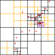
Figure 2: (a) A $\color[rgb]{0.75,0.30,0.15}2$-balanced quadtree on a set of points. True cells are shown in black, $\color[rgb]{0.75,0.30,0.15}B$-cells in yellow. (b) An insertion could cause a linear “cascade” of cells needing to be split if we want to maintain $\color[rgb]{0.75,0.30,0.15}2$-balance. Therefore, we only split the direct neighbors (purple), which may now be only $\color[rgb]{0.75,0.30,0.15}4$-balanced.

We will maintain the property that each true cell is $\color[rgb]{0.75,0.30,0.15}2$-balanced with respect to its larger neighbors, and every $\color[rgb]{0.75,0.30,0.15}B$-cell is $\color[rgb]{0.75,0.30,0.15}4$-balanced with respect to its larger neighbours.

Let $\color[rgb]{0.75,0.30,0.15}C$ be a true quadtree cell which is $\color[rgb]{0.75,0.30,0.15}2$-balanced with respect to its neighbors. When we split $\color[rgb]{0.75,0.30,0.15}C$, we examine the $\color[rgb]{0.75,0.30,0.15}3^{d}-1$ neighbors of $\color[rgb]{0.75,0.30,0.15}C$, and we split a larger neighbor $\color[rgb]{0.75,0.30,0.15}C^{\prime}$ if the children of $\color[rgb]{0.75,0.30,0.15}C$ are not $\color[rgb]{0.75,0.30,0.15}2$-balanced with respect to $\color[rgb]{0.75,0.30,0.15}C^{\prime}$. Thus we restore $\color[rgb]{0.75,0.30,0.15}2$-balance to $\color[rgb]{0.75,0.30,0.15}C$ at the cost of potentially inserting some $\color[rgb]{0.75,0.30,0.15}B$-cells which are only $\color[rgb]{0.75,0.30,0.15}4$-balanced, see Figure 2. However, it takes two operations to split a $\color[rgb]{0.75,0.30,0.15}B$-cell. First, we must insert a point into the $\color[rgb]{0.75,0.30,0.15}B$-cell, which does not require a split since the cell was already split to maintain balance. This changes the cell from a $\color[rgb]{0.75,0.30,0.15}B$-cell to a true cell. We also spend a constant amount of time examining each of the $\color[rgb]{0.75,0.30,0.15}O(1)$ neighbors of the newly true cell, and splitting them if necessary so that the cell is now $\color[rgb]{0.75,0.30,0.15}2$-balanced with respect to its neighbors.

We may be splitting a compressed node. Recall that if the size factor between a compressed node $\color[rgb]{0.75,0.30,0.15}v$ and it’s child $\color[rgb]{0.75,0.30,0.15}\tilde{v}$ is less than $\color[rgb]{0.75,0.30,0.15}a$, then we continue to split $\color[rgb]{0.75,0.30,0.15}v$ a constant number of times until the two components “grow together”. This case only requires a constant number of additional splits, and each split can be handled in worst-case $\color[rgb]{0.75,0.30,0.15}O(1)$ time as before. We maintain balance in the tree rooted at $\color[rgb]{0.75,0.30,0.15}\tilde{v}$ up to the level of $\color[rgb]{0.75,0.30,0.15}\tilde{v}$, which ensures that no nodes more than a constant factor smaller than $\color[rgb]{0.75,0.30,0.15}v$ are on the outside, and only $\color[rgb]{0.75,0.30,0.15}O(1)$ work needs to be done to rebalance the tree.

When we delete a $\color[rgb]{0.75,0.30,0.15}p$ from a cell $\color[rgb]{0.75,0.30,0.15}C$, we restore the quadtree to what it would be had $\color[rgb]{0.75,0.30,0.15}p$ never been inserted, essentially “undoing” the insertion of $\color[rgb]{0.75,0.30,0.15}p$. Since the original splitting and balancing only took $\color[rgb]{0.75,0.30,0.15}O(1)$ time, it clearly only takes $\color[rgb]{0.75,0.30,0.15}O(1)$ to undo that splitting and balancing. If $\color[rgb]{0.75,0.30,0.15}C$ was a $\color[rgb]{0.75,0.30,0.15}B$-cell, there is no change. If $\color[rgb]{0.75,0.30,0.15}C$ was a true cell, and its parent $\color[rgb]{0.75,0.30,0.15}\bar{C}$ has smaller neighbors which would become unbalanced if we merge $\color[rgb]{0.75,0.30,0.15}C$, then $\color[rgb]{0.75,0.30,0.15}\bar{C}$ may remain split and $\color[rgb]{0.75,0.30,0.15}C$ becomes a $\color[rgb]{0.75,0.30,0.15}B$-cell. Otherwise, we merge $\color[rgb]{0.75,0.30,0.15}C$.

Dynamic edge-oracle trees.

There have been several recent results which generalize classic one-dimensional dynamic structures to a multidimensional setting by combining classic techniques with a quadtree-style space decomposition. For example, the skip-quadtree [29] combines the quadtree and a skip-list, the quadtreap [56] combines a quadtree and a treap, and the splay quadtree combines a quadtree with a splay tree [59]. However, surprisingly there are no multidimensional data structures which incorporate finger searching techniques, i.e. structures that are able to support both logarithmic queries and worst-case constant time local updates on a quadtree. In the following we show how to build a dynamic edge-oracle tree which combines tree-decomposition and finger searching techniques with a quadtree to support $\color[rgb]{0.75,0.30,0.15}O(\log n)$ queries and $\color[rgb]{0.75,0.30,0.15}O(1)$ local updates.

Lemma 2.4.

If $\color[rgb]{0.75,0.30,0.15}v$ is a leaf in an unweighted free tree $\color[rgb]{0.75,0.30,0.15}T$, then the edge incident to $\color[rgb]{0.75,0.30,0.15}v$ has height $\color[rgb]{0.75,0.30,0.15}O(1)$ in the corresponding edge-oracle tree.

Proof 2.5.

Recall that we construct the static edge-oracle tree for $\color[rgb]{0.75,0.30,0.15}T$ by recursively locating an edge which divides $\color[rgb]{0.75,0.30,0.15}T$ into two components of approximately equal size. Thus the edges are split in order to maintain a balanced number of edges in each subtree of the edge-oracle tree. Since the edge adjacent to a leaf has 0 edges to one side of the split and at least one edge on the other side of the split, these edges will not be chosen for splitting by the algorithm until there are no other edge choices in the sub-tree.

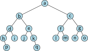
Figure 3: A not necessarily balanced or rooted abstract tree $\color[rgb]{0.75,0.30,0.15}T$ (a) and its corresponding edge-oracle tree (b). Labels on edges of $\color[rgb]{0.75,0.30,0.15}T$ match up with the label of the corresponding node in the edge-oracle tree. In the final structure we maintain the edge-oracle tree as a modified $\color[rgb]{0.75,0.30,0.15}(a,b)$-tree; small subtrees are maintained as buckets (linked-lists) to facilitate fast updates.

Lemma 2.6.

Let $\color[rgb]{0.75,0.30,0.15}T$ be a tree subject to dynamic insertions and deletions of leaves. We can maintain an edge-oracle tree over $\color[rgb]{0.75,0.30,0.15}T$ in $\color[rgb]{0.75,0.30,0.15}O(1)$ worst case time per local update.

Proof 2.7.

An insertion or deletion of a leaf and its associated edge in $\color[rgb]{0.75,0.30,0.15}T$ corresponds to an insertion or deletion of a node in the edge-oracle tree. Since the location of the node is known, and the height of the node is $\color[rgb]{0.75,0.30,0.15}O(1)$, we can borrow techniques from Fleischer [31] to perform updates in $\color[rgb]{0.75,0.30,0.15}O(1)$ time. The techniques are surprisingly simple, and we only sketch them here. We maintain the edge-oracle tree as an $\color[rgb]{0.75,0.30,0.15}(a,b)$-tree. However, we collapse each subtree of size $\color[rgb]{0.75,0.30,0.15}\Theta(\log n)$ into a single pseudo-node called a bucket. The original nodes within the bucket are maintained in a simple linked-list. When performing a query, we locate the correct bucket and iterate through the list for the correct original node in $\color[rgb]{0.75,0.30,0.15}O(\log n)$ time. Given a pointer to an original node, an update is simply a $\color[rgb]{0.75,0.30,0.15}O(1)$ linked-list operation. If many nodes are inserted into the same bucket, then a bucket may become too large. However, Fleischer shows how to distribute the rebuilding of buckets over later updates, only spending $\color[rgb]{0.75,0.30,0.15}O(1)$ time per update, such that the size of each bucket never deviates significantly from $\color[rgb]{0.75,0.30,0.15}\Theta(\log n)$.

Lemma 2.8.

In a quadtree, an edge-oracle can be simulated in $\color[rgb]{0.75,0.30,0.15}O(1)$ time.

Proof 2.9.

In a quadtree, we are searching for the quadtree leaf which contains a query point $\color[rgb]{0.75,0.30,0.15}q$. Each edge in a quadtree goes between a child cell and a parent cell that contains it. If the child cell contains the query point, then the leaf must be the child cell or one of its descendants, and the oracle returns the corresponding component of the quadtree. Otherwise, the oracle returns the other component of a quadtree. Since each quadtree cell is aware of its bounding box, we can compare the query point with the child cell and return our answer in constant time.

Lemma 2.10.

Let $\color[rgb]{0.75,0.30,0.15}P$ be a set of $\color[rgb]{0.75,0.30,0.15}n$ points, and $\color[rgb]{0.75,0.30,0.15}Q$ be a balanced and compressed quadtree on $\color[rgb]{0.75,0.30,0.15}P$. We can maintain $\color[rgb]{0.75,0.30,0.15}P$ and $\color[rgb]{0.75,0.30,0.15}Q$ in a data structure that supports $\color[rgb]{0.75,0.30,0.15}O(\log n)$ point location queries in $\color[rgb]{0.75,0.30,0.15}Q$, and local insertions and deletions of points in $\color[rgb]{0.75,0.30,0.15}P$ (i.e., when given the corresponding cells of $\color[rgb]{0.75,0.30,0.15}Q$) in $\color[rgb]{0.75,0.30,0.15}O(1)$ time.

Proof 2.11.

By Lemmas 2.6 and 2.8, we can maintain an edge-oracle tree over the compressed quadtree which can find the unique quadtree cell containing a query point in $\color[rgb]{0.75,0.30,0.15}O(\log n)$ time and respond to local updates in the quadtree in $\color[rgb]{0.75,0.30,0.15}O(1)$ time.

Marked-ancestor trees.

We show how to answer marked-ancestor queries on a pointer-machine. Details are given in Section C.2.

Lemma 2.12.

We can maintain a data structure over any rooted tree $\color[rgb]{0.75,0.30,0.15}T$ which supports insertions and deletions of leaves in $\color[rgb]{0.75,0.30,0.15}O(1)$ amortized time, marking and unmarking nodes in $\color[rgb]{0.75,0.30,0.15}O(\log\log n)$ worst-case time, and queries for the lowest marked ancestor in $\color[rgb]{0.75,0.30,0.15}O(\log n)$ worst-case time. All operations are supported on a pointer machine.

3 One-Dimensional Case

To aid our exposition, we first present a solution to the one-dimensional version of the problem. Our data structure illustrates the key ideas of our approach while being significantly simpler than the two-dimensional version. Note that in $\color[rgb]{0.75,0.30,0.15}\mathbb{R}^{1}$, our input set $\color[rgb]{0.75,0.30,0.15}\mathcal{R}$ of geometric regions is a set of non-overlapping intervals. The difficulty of the problem comes from the fact that a local update may replace any interval by another interval of similar size at a distance related to that size; hence, it may “jump” over an arbitrary number of smaller intervals. Our solution works on a pure Real-valued pointer machine, and achieves constant time updates.

3.1 Definition of the data structure

Our data structure consists of two trees. The first is designed to facilitate efficient updates and the second is designed to facilitate efficient queries. The update tree is a compressed quadtree on the center points of the intervals; The quadtree stores a pointer to each interval in the leaf that contains its center point. We also augment the tree with level-links, so that each cell has a pointer to its adjacent cells of the same size (if they exist), and maintain balance in the quadtree as described in Lemma 2.2. The leaves of the quadtree induce a linear size subdivision of the real line; the query tree is a search tree over this subdivision that allows for fast point location and constant time local updates. We also maintain pointers between the leaves of the two trees, so that when we perform a point location query in the query tree, we also get a pointer to the corresponding cell in the quadtree, and given any leaf in the quadtree, we have a pointer to the corresponding leaf in the query tree. Figure 4 illustrates the data structure.

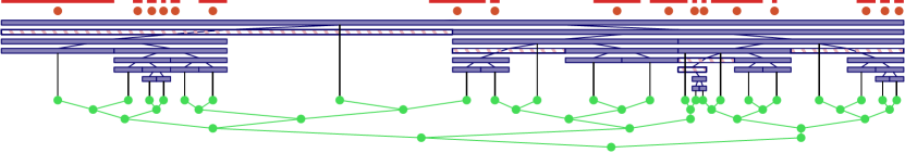
Figure 4: A set of disjoint intervals and their center points (red); a compressed quadtree on the center points (blue); and a search tree on the leaves (or parts of internal cells not covered by children) of the quadtree (green).

Lemma 3.1.

Let $\color[rgb]{0.75,0.30,0.15}I\in\mathcal{R}$ be an interval, and let $\color[rgb]{0.75,0.30,0.15}I^{\prime}$ be another interval that is $\color[rgb]{0.75,0.30,0.15}O(\rho)$-similar to $\color[rgb]{0.75,0.30,0.15}I$. Suppose we are given a quadtree storing the midpoints of the intervals in $\color[rgb]{0.75,0.30,0.15}\mathcal{R}$ and a pointer to the leaf containing the midpoint of $\color[rgb]{0.75,0.30,0.15}I$. Then we can find the leaf which contains the midpoint of $\color[rgb]{0.75,0.30,0.15}I^{\prime}$ in $\color[rgb]{0.75,0.30,0.15}O(\log\rho)$ time.

Proof 3.2.

Let $\color[rgb]{0.75,0.30,0.15}C$ be the quadtree leaf cell which contains the center point of $\color[rgb]{0.75,0.30,0.15}I$, and let $\color[rgb]{0.75,0.30,0.15}C^{\prime}$ be the quadtree cell which contains the center point of $\color[rgb]{0.75,0.30,0.15}I^{\prime}$. Observe that $\color[rgb]{0.75,0.30,0.15}I$ is at most four times as large as $\color[rgb]{0.75,0.30,0.15}C$: otherwise, $\color[rgb]{0.75,0.30,0.15}I$ would completely cover the parent $\color[rgb]{0.75,0.30,0.15}\tilde{C}$ of $\color[rgb]{0.75,0.30,0.15}C$, but then no other intervals could have their center points in $\color[rgb]{0.75,0.30,0.15}\tilde{C}$ to cause $\color[rgb]{0.75,0.30,0.15}\tilde{C}$ to be split. Similarly, $\color[rgb]{0.75,0.30,0.15}I^{\prime}$ is at most four times as large as the new quadtree cell $\color[rgb]{0.75,0.30,0.15}C^{\prime}$. Therefore, the distance between $\color[rgb]{0.75,0.30,0.15}I$ and $\color[rgb]{0.75,0.30,0.15}I^{\prime}$ is proportional to the size of $\color[rgb]{0.75,0.30,0.15}C$ (and $\color[rgb]{0.75,0.30,0.15}C^{\prime}$). Since we maintain balance in the quadtree according to Lemma 2.2, we can find $\color[rgb]{0.75,0.30,0.15}C^{\prime}$ from $\color[rgb]{0.75,0.30,0.15}C$ by following $\color[rgb]{0.75,0.30,0.15}O(1)$ level-link and parent-child pointers in the quadtree.

3.2 Handling queries

In a query, we are given a point $\color[rgb]{0.75,0.30,0.15}q$ and must return the interval in $\color[rgb]{0.75,0.30,0.15}\mathcal{R}$ that contains $\color[rgb]{0.75,0.30,0.15}q$. We search in the query tree to find the quadtree leaf cell which contains $\color[rgb]{0.75,0.30,0.15}q$ and its two neighboring cells in $\color[rgb]{0.75,0.30,0.15}O(\log n)$ time. Any interval $\color[rgb]{0.75,0.30,0.15}I$ which overlaps $\color[rgb]{0.75,0.30,0.15}q$ must have its center point in one of these three cells (otherwise, there would be an empty cell between the cell containing $\color[rgb]{0.75,0.30,0.15}q$ and the cell containing the center point of $\color[rgb]{0.75,0.30,0.15}I$). We compare $\color[rgb]{0.75,0.30,0.15}q$ with the intervals stored at these cells (if any) to find the unique interval that contains $\color[rgb]{0.75,0.30,0.15}q$ or report that there is no containing interval in $\color[rgb]{0.75,0.30,0.15}O(1)$ time. Thus the total time required by a query is $\color[rgb]{0.75,0.30,0.15}O(\log n)$.

3.3 Handling updates

In an update, we are given a pointer to an interval $\color[rgb]{0.75,0.30,0.15}I\in\mathcal{R}$, and a new interval $\color[rgb]{0.75,0.30,0.15}I^{\prime}$ that should replace $\color[rgb]{0.75,0.30,0.15}I$. We follow pointers in the quadtree to find the new cell which contains the center point. If $\color[rgb]{0.75,0.30,0.15}I$ and $\color[rgb]{0.75,0.30,0.15}I^{\prime}$ are $\color[rgb]{0.75,0.30,0.15}O(1)$-similar, Lemma 3.1 implies that the new cell is at most a constant number of cells away, and we find the correct cell in $\color[rgb]{0.75,0.30,0.15}O(1)$ time. Then we remove the center point from the old cell and insert it into the new cell, performing any compression or decompression required in the quadtree. This only requires a constant number of pointer changes in the quadtree and can be done in $\color[rgb]{0.75,0.30,0.15}O(1)$ worst-case time, and we may also need to restore balance to the quadtree, which requires $\color[rgb]{0.75,0.30,0.15}O(1)$ worst-case time by Lemma 2.2. Finally, we follow pointers from the quadtree to the query tree, and perform the corresponding deletion and insertion in that tree, which by Lemma 2.10 takes only constant time. Thus, the entire update can be completed in $\color[rgb]{0.75,0.30,0.15}O(1)$ worst-case time.

Note that we can also insert or delete intervals from the data structure in $\color[rgb]{0.75,0.30,0.15}O(\log n)$ time; we perform a query to locate where the interval belongs and a local update to insert it or remove it.

Theorem 3.3.

We can maintain a linear size data structure over a set of $\color[rgb]{0.75,0.30,0.15}n$ non-overlapping intervals such that we can perform point location queries and insertion and deletion of intervals in $\color[rgb]{0.75,0.30,0.15}O(\log n)$ worst-case time and local updates in $\color[rgb]{0.75,0.30,0.15}O(\log\rho)$ worst-case time.

4 Two-Dimensional Case

We now focus our attention on disjoint fat regions in the plane. Intuitively, a fat region should not have any long skinny pieces. We consider two types of fat regions which precisely capture this intuition: thick convex regions and wide polygons. We say $\color[rgb]{0.75,0.30,0.15}R$ is $\color[rgb]{0.75,0.30,0.15}\beta$-thick if there exists a pair of concentric balls $\color[rgb]{0.75,0.30,0.15}I,O$ with $\color[rgb]{0.75,0.30,0.15}I\subseteq R\subseteq O$ and $\color[rgb]{0.75,0.30,0.15}|O|\leq\beta|I|$, see Figure 5. Let $\color[rgb]{0.75,0.30,0.15}\delta\geq 1$. A $\color[rgb]{0.75,0.30,0.15}\delta$-corridor is a isosceles trapezoid whose slanted edges are at most $\color[rgb]{0.75,0.30,0.15}\delta$ times as long as its base. A simple polygon $\color[rgb]{0.75,0.30,0.15}P$ is $\color[rgb]{0.75,0.30,0.15}\delta$-wide if any isosceles trapezoid $\color[rgb]{0.75,0.30,0.15}T\subset P$ whose slanted edges lie on the boundary of $\color[rgb]{0.75,0.30,0.15}P$ is a $\color[rgb]{0.75,0.30,0.15}\delta$-corridor [64], see Figure 5. Note that any $\color[rgb]{0.75,0.30,0.15}\delta$-wide polygon $\color[rgb]{0.75,0.30,0.15}R$ of constant complexity is also $\color[rgb]{0.75,0.30,0.15}\beta$-thick, with $\color[rgb]{0.75,0.30,0.15}\beta\in\Theta(\delta)$.

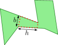
Figure 5: (a) A $\color[rgb]{0.75,0.30,0.15}\beta$-thick region for $\color[rgb]{0.75,0.30,0.15}\beta=\frac{r_{O}}{r_{I}}$. (b) A $\color[rgb]{0.75,0.30,0.15}\delta$-wide region for $\color[rgb]{0.75,0.30,0.15}\delta=h/b$.

We will first solve the problem for convex thick regions, and then extend the result to non-convex wide polygons. Analogously to the 1D case, we will store for each region $\color[rgb]{0.75,0.30,0.15}R\in\cal R$ a representative point $\color[rgb]{0.75,0.30,0.15}p$ that lies somehow “in the middle” of $\color[rgb]{0.75,0.30,0.15}R$. When the regions are $\color[rgb]{0.75,0.30,0.15}\beta$-thick, we will use the center point of the two concentric disks from the thickness definition as representative point. We denote the set of representative points of the regions in $\color[rgb]{0.75,0.30,0.15}\mathcal{R}$ by $\color[rgb]{0.75,0.30,0.15}P$. Let $\color[rgb]{0.75,0.30,0.15}T$ be the quadtree built over $\color[rgb]{0.75,0.30,0.15}P$. We distinguish between true cells, which are necessary in any valid compressed quadtree over $\color[rgb]{0.75,0.30,0.15}P$, and $\color[rgb]{0.75,0.30,0.15}B$-cells, which may further subdivide a true cell and are only added in order to maintain balance. We store each representative point $\color[rgb]{0.75,0.30,0.15}m$ in $\color[rgb]{0.75,0.30,0.15}T$ according to the following rule: Let $\color[rgb]{0.75,0.30,0.15}C_{v}$ be the smallest quadtree cell containing $\color[rgb]{0.75,0.30,0.15}m$. If $\color[rgb]{0.75,0.30,0.15}C_{v}$ is a true cell, then $\color[rgb]{0.75,0.30,0.15}m$ is stored in $\color[rgb]{0.75,0.30,0.15}v$. If $\color[rgb]{0.75,0.30,0.15}C_{v}$ is a $\color[rgb]{0.75,0.30,0.15}B$-cell, then $\color[rgb]{0.75,0.30,0.15}m$ is stored in $\color[rgb]{0.75,0.30,0.15}u$, the lowest (not necessarily proper) ancestor of $\color[rgb]{0.75,0.30,0.15}v$ in $\color[rgb]{0.75,0.30,0.15}T$ such that $\color[rgb]{0.75,0.30,0.15}|C_{u}|\geq|R|/(4\beta)$.

Several new problems are introduced which were not present in the 1D case. We briefly sketch how to address each of these problems, and then present the complete solution.

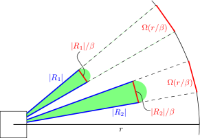
Figure 6: (a) The intersecting region could be stored a linear distance from the query cell (containing the blue point). (b) The number of regions which can intersect quadtree leaf $\color[rgb]{0.75,0.30,0.15}C$ is at most $\color[rgb]{0.75,0.30,0.15}O(\beta)$, since each region blocks a $\color[rgb]{0.75,0.30,0.15}\Omega(1/\beta)$ fraction of a large circle centered at $\color[rgb]{0.75,0.30,0.15}C$, by similar triangles.

Linear distance.

When performing a query in the one-dimensional case, the location in the quadtree of any intersecting region is at most a constant number of cells away. However, in the two-dimensional case, the location of an intersecting region may be up to a linear number of cells away, as shown in Figure 6. We solve this problem with some additional bookkeeping. Given a quadtree cell $\color[rgb]{0.75,0.30,0.15}C_{q}$, we use two different strategies to locate regions intersecting $\color[rgb]{0.75,0.30,0.15}C_{q}$ depending on their size. All regions of size at least $\color[rgb]{0.75,0.30,0.15}2\beta|C_{q}|$ will be located using a marked-ancestor data structure: an additional search structure which we explain in more detail below. All regions of size less than $\color[rgb]{0.75,0.30,0.15}2\beta|C_{q}|$ which intersect $\color[rgb]{0.75,0.30,0.15}C_{q}$ will register a bidirectional pointer with $\color[rgb]{0.75,0.30,0.15}C_{q}$ using the following tagging strategy.

Let $\color[rgb]{0.75,0.30,0.15}d$ be the smallest diameter of a quadtree cell such that $\color[rgb]{0.75,0.30,0.15}d\geq|R|/(4\beta)$. Let $\color[rgb]{0.75,0.30,0.15}S_{R}$ be the set of quadtree cells $\color[rgb]{0.75,0.30,0.15}C$ which intersect $\color[rgb]{0.75,0.30,0.15}R$ and are either a leaf or have size $\color[rgb]{0.75,0.30,0.15}|C|=d$. All cells in $\color[rgb]{0.75,0.30,0.15}S_{R}$ will be tagged with a pointer to $\color[rgb]{0.75,0.30,0.15}R$. Since the quadtree is balanced, given a pointer to any cell in $\color[rgb]{0.75,0.30,0.15}S_{R}$, we can locate all cells in $\color[rgb]{0.75,0.30,0.15}S_{R}$ in $\color[rgb]{0.75,0.30,0.15}O(|S_{R}|)$ time. By the following lemma, $\color[rgb]{0.75,0.30,0.15}S_{R}$ must contain the cell containing the representative point of $\color[rgb]{0.75,0.30,0.15}R$.

Lemma 4.1.

Let $\color[rgb]{0.75,0.30,0.15}R$ be a $\color[rgb]{0.75,0.30,0.15}\beta$-thick region stored by our data structure. If $\color[rgb]{0.75,0.30,0.15}C$ is the quadtree cell which stores the representative point of $\color[rgb]{0.75,0.30,0.15}R$, then $\color[rgb]{0.75,0.30,0.15}C$ has side length at least $\color[rgb]{0.75,0.30,0.15}\frac{|R|}{4\beta}$.

Proof 4.2.

If $\color[rgb]{0.75,0.30,0.15}C$ is a $\color[rgb]{0.75,0.30,0.15}B$-cell, then the claim is true by construction. Suppose $\color[rgb]{0.75,0.30,0.15}C$ is a true cell. Let $\color[rgb]{0.75,0.30,0.15}m$ be the representative point of $\color[rgb]{0.75,0.30,0.15}R$. By the definition of thickness, there exists a disk $\color[rgb]{0.75,0.30,0.15}I\subseteq R$ centered at $\color[rgb]{0.75,0.30,0.15}m$ with $\color[rgb]{0.75,0.30,0.15}|I|\geq|R|/\beta$. $\color[rgb]{0.75,0.30,0.15}I$ contains no representative points of regions other than $\color[rgb]{0.75,0.30,0.15}R$. Let $\color[rgb]{0.75,0.30,0.15}C$ be the cell containing $\color[rgb]{0.75,0.30,0.15}m$. Note that if $\color[rgb]{0.75,0.30,0.15}C$ contains $\color[rgb]{0.75,0.30,0.15}m$ and is significantly smaller than $\color[rgb]{0.75,0.30,0.15}|R|$, then $\color[rgb]{0.75,0.30,0.15}C$ must be completely contained in $\color[rgb]{0.75,0.30,0.15}I$. However, $\color[rgb]{0.75,0.30,0.15}C$ must be the largest quadtree cell completely contained in $\color[rgb]{0.75,0.30,0.15}I$, since if the parent $\color[rgb]{0.75,0.30,0.15}\bar{C}$ of $\color[rgb]{0.75,0.30,0.15}C$ in the quadtree is completely contained in $\color[rgb]{0.75,0.30,0.15}R$, then $\color[rgb]{0.75,0.30,0.15}\bar{C}$ would not have been further subdivided because $\color[rgb]{0.75,0.30,0.15}\bar{C}$ would contain no other points. Therefore, $\color[rgb]{0.75,0.30,0.15}\bar{C}$ must have some portion outside of $\color[rgb]{0.75,0.30,0.15}I$ and must have size larger than $\color[rgb]{0.75,0.30,0.15}|I|/2$. Thus the size of $\color[rgb]{0.75,0.30,0.15}C$ is at least $\color[rgb]{0.75,0.30,0.15}|I|/4\geq|R|/(4\beta)$.

Moreover, by the following lemma $\color[rgb]{0.75,0.30,0.15}|S_{R}|=O(\beta)$, and therefore, given the cell containing the representative point of $\color[rgb]{0.75,0.30,0.15}R$ we can tag all cells in $\color[rgb]{0.75,0.30,0.15}S_{R}$ in $\color[rgb]{0.75,0.30,0.15}O(\beta)$ time.

Lemma 4.3.

Let $\color[rgb]{0.75,0.30,0.15}R$ be a $\color[rgb]{0.75,0.30,0.15}\beta$-thick region stored in our data structure, and let $\color[rgb]{0.75,0.30,0.15}C$ be quadtree cell that stores the representative point of $\color[rgb]{0.75,0.30,0.15}R$. Then there are at most $\color[rgb]{0.75,0.30,0.15}O(\beta)$ quadtree cells of size $\color[rgb]{0.75,0.30,0.15}|C|$ required to cover $\color[rgb]{0.75,0.30,0.15}R$.

Proof 4.4.

Let $\color[rgb]{0.75,0.30,0.15}I$ be the largest inscribed disk of $\color[rgb]{0.75,0.30,0.15}R$. The boundary of $\color[rgb]{0.75,0.30,0.15}I$ touches the boundary of $\color[rgb]{0.75,0.30,0.15}R$ in two or three points. If two points, then these are diametral on $\color[rgb]{0.75,0.30,0.15}I$, so $\color[rgb]{0.75,0.30,0.15}R$ is contained in a strip of width $\color[rgb]{0.75,0.30,0.15}|I|$. If three points, then take the diametral points of these three points and take the strips of width $\color[rgb]{0.75,0.30,0.15}|I|$ of these three pairs; $\color[rgb]{0.75,0.30,0.15}R$ is contained in the union of these three strips. Now, if $\color[rgb]{0.75,0.30,0.15}R$ is beta-thick, the portion of the strips it can be in is at most $\color[rgb]{0.75,0.30,0.15}\beta|I|$ long. So, $\color[rgb]{0.75,0.30,0.15}R$ can be covered by $\color[rgb]{0.75,0.30,0.15}O(\beta)$ disks the size of $\color[rgb]{0.75,0.30,0.15}I$. Each such disk can be covered by at most $\color[rgb]{0.75,0.30,0.15}O(1)$ cells of size $\color[rgb]{0.75,0.30,0.15}|C|$, by Lemma 4.1. Thus, $\color[rgb]{0.75,0.30,0.15}O(\beta)$ cells are required to cover $\color[rgb]{0.75,0.30,0.15}R$.

Linear overlap.

In the one-dimensional case, we store only the center points of our regions, and the number of regions that overlap any quadtree cell is at most three. In two dimensions, it appears that we may have a large number of small regions that intersect a quadtree cell. However, we show in the following lemma that this is not the case.

Lemma 4.5.

The number of $\color[rgb]{0.75,0.30,0.15}\beta$-thick convex regions intersecting any balanced quadtree leaf is $\color[rgb]{0.75,0.30,0.15}O(\beta)$.

Proof 4.6.

Let $\color[rgb]{0.75,0.30,0.15}R_{C}$ be the set of thick convex regions that intersect the boundary of leaf $\color[rgb]{0.75,0.30,0.15}C$, and let $\color[rgb]{0.75,0.30,0.15}r$ be the radius of a large disk $\color[rgb]{0.75,0.30,0.15}D$ containing all regions in $\color[rgb]{0.75,0.30,0.15}R_{C}$. For each region $\color[rgb]{0.75,0.30,0.15}R_{j}\in R_{C}$ there exists a disk $\color[rgb]{0.75,0.30,0.15}I_{j}\subseteq R_{j}$ with center $\color[rgb]{0.75,0.30,0.15}m_{j}$ such that $\color[rgb]{0.75,0.30,0.15}|I_{j}|\geq|R_{j}|/\beta$. Moreover, since each region $\color[rgb]{0.75,0.30,0.15}R_{j}$ is convex, it must contain a triangle consisting of the diameter of $\color[rgb]{0.75,0.30,0.15}I_{j}$ and some point $\color[rgb]{0.75,0.30,0.15}p_{j}\in R_{j}\cap C$. Each of the four sides of $\color[rgb]{0.75,0.30,0.15}C$ can “see” at most $\color[rgb]{0.75,0.30,0.15}\pi r$ of the perimeter of $\color[rgb]{0.75,0.30,0.15}D$. However, by a similar triangles argument each triangle must block the line of sight from one or more sides to at least $\color[rgb]{0.75,0.30,0.15}\Theta(r/\beta)$ of the perimeter (see Figure 6). Thus, since the regions are convex and disjoint, the number of regions in $\color[rgb]{0.75,0.30,0.15}R_{C}$ is at most $\color[rgb]{0.75,0.30,0.15}O(\beta)$.

4.1 Definition of the data structure

At the core, our data structure is similar to the one-dimensional data structure described above: we have a spacial tree, which allows for efficient updates, and a search tree, which allows for efficient searching over the quadtree. However, our data structure is augmented to address the problems introduced by the two-dimensional case. We maintain a dynamic balanced quadtree $\color[rgb]{0.75,0.30,0.15}Q$ over $\color[rgb]{0.75,0.30,0.15}P$, which we augment to support mark and unmark operations and marked-ancestor queries, and we maintain a dynamic edge-oracle tree on the edges of $\color[rgb]{0.75,0.30,0.15}Q$.

Marked-ancestor tree.

Suppose we are given an angle $\color[rgb]{0.75,0.30,0.15}\phi$ which divides $\color[rgb]{0.75,0.30,0.15}2\pi$ (i.e., $\color[rgb]{0.75,0.30,0.15}k\phi=2\pi$), and consider the set of angular intervals $\color[rgb]{0.75,0.30,0.15}\Phi_{i}=[i\phi,(i+1)\phi]$ (modulo $\color[rgb]{0.75,0.30,0.15}2\pi$), for integers $\color[rgb]{0.75,0.30,0.15}1\leq i\leq k$. For each quadtree cell $\color[rgb]{0.75,0.30,0.15}C$ of $\color[rgb]{0.75,0.30,0.15}Q$ with center point $\color[rgb]{0.75,0.30,0.15}c$, we define the wedge $\color[rgb]{0.75,0.30,0.15}W_{C}^{i}$ centered at $\color[rgb]{0.75,0.30,0.15}c$ and with opening angle $\color[rgb]{0.75,0.30,0.15}\phi$ to be the union of all halflines from $\color[rgb]{0.75,0.30,0.15}c$ in a direction in $\color[rgb]{0.75,0.30,0.15}\Phi_{i}$. Let $\color[rgb]{0.75,0.30,0.15}{\cal W}_{C}=\{W_{C}^{i}\mid 1\leq i\leq k\}$; note that $\color[rgb]{0.75,0.30,0.15}{\cal W}_{C}$ partitions $\color[rgb]{0.75,0.30,0.15}\mathbb{R}^{2}$ into $\color[rgb]{0.75,0.30,0.15}k$ wedges.

For each $\color[rgb]{0.75,0.30,0.15}1\leq i\leq k$, let $\color[rgb]{0.75,0.30,0.15}T_{i}$ be a marked-ancestor structure on $\color[rgb]{0.75,0.30,0.15}Q$. We mark a cell $\color[rgb]{0.75,0.30,0.15}C$ in $\color[rgb]{0.75,0.30,0.15}T_{i}$ if and only if there is a region $\color[rgb]{0.75,0.30,0.15}R\in\cal R$ of size $\color[rgb]{0.75,0.30,0.15}2\beta|C|\leq|R|<4\beta|C|$ that intersects $\color[rgb]{0.75,0.30,0.15}C$, and such that the center point of $\color[rgb]{0.75,0.30,0.15}R$ lies in $\color[rgb]{0.75,0.30,0.15}W_{C}^{i}$.

When doing a query, we will only look at the first marked ancestor in each $\color[rgb]{0.75,0.30,0.15}T_{i}$. Lemma 4.8 captures the essential property of the regions which enables this strategy. First, we need the following claim.

Claim 1.

Let $\color[rgb]{0.75,0.30,0.15}\beta$ be given and set $\color[rgb]{0.75,0.30,0.15}\phi=\frac{2\pi}{\lceil 13\beta\rceil}$. Let $\color[rgb]{0.75,0.30,0.15}C$ be a cell that is marked in $\color[rgb]{0.75,0.30,0.15}T_{i}$ by a $\color[rgb]{0.75,0.30,0.15}\beta$-thick region $\color[rgb]{0.75,0.30,0.15}R$. Let $\color[rgb]{0.75,0.30,0.15}L_{C}^{i}$ be the set of lines that start in $\color[rgb]{0.75,0.30,0.15}C$, and have a direction in $\color[rgb]{0.75,0.30,0.15}\Phi_{i}$. Then every line in $\color[rgb]{0.75,0.30,0.15}L_{C}^{i}$ intersects $\color[rgb]{0.75,0.30,0.15}R$.

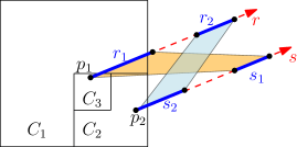
Figure 7: (a) Illustration of Claim 1. (b) Illustration of Lemma 4.8.

Proof 4.7.

Let $\color[rgb]{0.75,0.30,0.15}m$ be the representative point of $\color[rgb]{0.75,0.30,0.15}R$. Since $\color[rgb]{0.75,0.30,0.15}R$ is $\color[rgb]{0.75,0.30,0.15}\beta$-thick, there exist disks $\color[rgb]{0.75,0.30,0.15}I\subseteq R\subseteq O$ centered at $\color[rgb]{0.75,0.30,0.15}m$ with $\color[rgb]{0.75,0.30,0.15}|O|/|I|\leq\beta$. Since $\color[rgb]{0.75,0.30,0.15}R$ caused $\color[rgb]{0.75,0.30,0.15}C$ to be marked, $\color[rgb]{0.75,0.30,0.15}O$, must intersect $\color[rgb]{0.75,0.30,0.15}C$, and $\color[rgb]{0.75,0.30,0.15}m$ must lie in $\color[rgb]{0.75,0.30,0.15}W_{C}^{i}$. See Figure 7.

Now, we need that $\color[rgb]{0.75,0.30,0.15}I$ intersects all lines in $\color[rgb]{0.75,0.30,0.15}L_{C}^{i}$. The distance from $\color[rgb]{0.75,0.30,0.15}m$ to $\color[rgb]{0.75,0.30,0.15}C$ is at most $\color[rgb]{0.75,0.30,0.15}\frac{1}{2}|O|\leq\frac{\beta}{2}|I|$. Then, the distance from $\color[rgb]{0.75,0.30,0.15}m$ to the far edge of $\color[rgb]{0.75,0.30,0.15}W_{C}^{i}$ is at most $\color[rgb]{0.75,0.30,0.15}\frac{\beta}{2}|I|\sin\phi$, and the distance to the far edge of $\color[rgb]{0.75,0.30,0.15}L_{C}^{i}$ is at most $\color[rgb]{0.75,0.30,0.15}\frac{\beta}{2}|I|\sin\phi+\frac{1}{2}|C|$. Since $\color[rgb]{0.75,0.30,0.15}|R|\geq 2\beta|C|$, we know that $\color[rgb]{0.75,0.30,0.15}|C|\leq\frac{1}{2}|I|$. Using $\color[rgb]{0.75,0.30,0.15}\phi=\frac{2\pi}{13\beta}$ implies $\color[rgb]{0.75,0.30,0.15}\beta\sin\phi\leq\frac{2\pi}{13}<\frac{1}{2}$. Combining these, we see that $\color[rgb]{0.75,0.30,0.15}|I|\geq\beta|I|\sin\phi+|C|$, so, $\color[rgb]{0.75,0.30,0.15}I$ blocks all lines in $\color[rgb]{0.75,0.30,0.15}L_{C}^{i}$.

Lemma 4.8.

Let $\color[rgb]{0.75,0.30,0.15}C_{1}$ be a cell that is marked in $\color[rgb]{0.75,0.30,0.15}T_{i}$ by a convex and $\color[rgb]{0.75,0.30,0.15}\beta$-thick region $\color[rgb]{0.75,0.30,0.15}R_{1}$, and let $\color[rgb]{0.75,0.30,0.15}C_{2}$ be a descendant of $\color[rgb]{0.75,0.30,0.15}C_{1}$ that is marked in $\color[rgb]{0.75,0.30,0.15}T_{i}$ by a convex and $\color[rgb]{0.75,0.30,0.15}\beta$-thick region $\color[rgb]{0.75,0.30,0.15}R_{2}$. Then there cannot be a descendant $\color[rgb]{0.75,0.30,0.15}C_{3}$ of $\color[rgb]{0.75,0.30,0.15}C_{2}$ that intersects $\color[rgb]{0.75,0.30,0.15}R_{1}$.

Proof 4.9.

Let $\color[rgb]{0.75,0.30,0.15}R_{2}$ and $\color[rgb]{0.75,0.30,0.15}R_{1}$ be convex fat regions which mark cells $\color[rgb]{0.75,0.30,0.15}C_{2}$ and $\color[rgb]{0.75,0.30,0.15}C_{1}$ respectively. Then there is a point $\color[rgb]{0.75,0.30,0.15}p_{2}\in R_{2}\cap C_{2}$. Suppose for contradiction that $\color[rgb]{0.75,0.30,0.15}R_{1}$ intersects $\color[rgb]{0.75,0.30,0.15}C_{3}$; that is, there exists a point $\color[rgb]{0.75,0.30,0.15}p_{1}\in R_{1}\cap C_{3}$. Let $\color[rgb]{0.75,0.30,0.15}r$ and $\color[rgb]{0.75,0.30,0.15}s$ be two parallel rays from $\color[rgb]{0.75,0.30,0.15}p_{1}$ and $\color[rgb]{0.75,0.30,0.15}p_{2}$ in some direction $\color[rgb]{0.75,0.30,0.15}\phi\in\Phi_{i}$. Note that rays $\color[rgb]{0.75,0.30,0.15}r$ and $\color[rgb]{0.75,0.30,0.15}s$ are both in $\color[rgb]{0.75,0.30,0.15}L_{C_{2}}^{i}$. Therefore each ray must intersect both $\color[rgb]{0.75,0.30,0.15}R_{1}$ and $\color[rgb]{0.75,0.30,0.15}R_{2}$ by Claim 1. Since each region $\color[rgb]{0.75,0.30,0.15}R_{1}$ and $\color[rgb]{0.75,0.30,0.15}R_{2}$ is convex, their intersection with each ray $\color[rgb]{0.75,0.30,0.15}r$ (or $\color[rgb]{0.75,0.30,0.15}s$) is a single line segment, denoted $\color[rgb]{0.75,0.30,0.15}r_{1}$ and $\color[rgb]{0.75,0.30,0.15}r_{2}$ ($\color[rgb]{0.75,0.30,0.15}s_{1}$ and $\color[rgb]{0.75,0.30,0.15}s_{2}$) respectively. Moreover, since $\color[rgb]{0.75,0.30,0.15}R_{1}$ and $\color[rgb]{0.75,0.30,0.15}R_{2}$ are disjoint, the segments $\color[rgb]{0.75,0.30,0.15}r_{1}$ and $\color[rgb]{0.75,0.30,0.15}r_{2}$ ($\color[rgb]{0.75,0.30,0.15}s_{1}$ and $\color[rgb]{0.75,0.30,0.15}s_{2}$) are also disjoint (see Figure 7).

Since $\color[rgb]{0.75,0.30,0.15}p_{1}\in R_{1}$, $\color[rgb]{0.75,0.30,0.15}r_{1}$ must come before $\color[rgb]{0.75,0.30,0.15}r_{2}$ on the ray $\color[rgb]{0.75,0.30,0.15}r$. Similarly, $\color[rgb]{0.75,0.30,0.15}s_{2}$ must come before $\color[rgb]{0.75,0.30,0.15}s_{1}$ on the ray $\color[rgb]{0.75,0.30,0.15}s$. Moreover, $\color[rgb]{0.75,0.30,0.15}R_{1}$ is convex, and thus the convex quadrilateral defined by $\color[rgb]{0.75,0.30,0.15}r_{1},s_{1}$ is completely contained in $\color[rgb]{0.75,0.30,0.15}R_{1}$, and likewise $\color[rgb]{0.75,0.30,0.15}r_{2},s_{2}\subseteq R_{2}$. These two quadrilaterals must intersect, which is a contradiction because $\color[rgb]{0.75,0.30,0.15}R_{1}$ and $\color[rgb]{0.75,0.30,0.15}R_{2}$ are disjoint. Therefore there is no point $\color[rgb]{0.75,0.30,0.15}p_{1}\in R_{1}\cap C_{3}$.

4.2 Handling queries

Given a query point $\color[rgb]{0.75,0.30,0.15}q$, we want to find out which region (if any) contains $\color[rgb]{0.75,0.30,0.15}q$. We begin by performing a point location query for $\color[rgb]{0.75,0.30,0.15}q$ in the quadtree $\color[rgb]{0.75,0.30,0.15}Q$. By Lemma 2.10 we can find the leaf cell $\color[rgb]{0.75,0.30,0.15}C$ in the quadtree which contains $\color[rgb]{0.75,0.30,0.15}q$ in $\color[rgb]{0.75,0.30,0.15}O(\log n)$ time using the edge-oracle tree.

By Lemma 4.5, there can only be $\color[rgb]{0.75,0.30,0.15}O(\beta)$ regions which intersect $\color[rgb]{0.75,0.30,0.15}C$. All regions of size at most $\color[rgb]{0.75,0.30,0.15}2\beta|C|$ will have tagged $\color[rgb]{0.75,0.30,0.15}C$ with a pointer to themselves, and are immediately available from $\color[rgb]{0.75,0.30,0.15}C$. Moreover, we can find all regions of size at least $\color[rgb]{0.75,0.30,0.15}2\beta|C|$ in $\color[rgb]{0.75,0.30,0.15}O(\beta\log n)$ time by querying the marked-ancestor structures. We compare each region to our query point, and determine which region (if any) intersects the query point in $\color[rgb]{0.75,0.30,0.15}O(\beta)$ time. Thus, we can answer the query in total time $\color[rgb]{0.75,0.30,0.15}O(\beta\log n)$.

4.3 Handling updates

We only store the representative points of the regions in the quadtree. Thus, when performing a local update, it is sufficient to find the new location for the region’s representative point, and then update the quadtree, tags, marked-ancestor trees, and edge-oracle trees accordingly.

Locating the new representative point.

Given a pointer to a region $\color[rgb]{0.75,0.30,0.15}R$, we replace it by another region $\color[rgb]{0.75,0.30,0.15}R^{\prime}$ that is $\color[rgb]{0.75,0.30,0.15}\rho$-similar to $\color[rgb]{0.75,0.30,0.15}R$ for any arbitrary parameter $\color[rgb]{0.75,0.30,0.15}\rho\geq 1$. Let $\color[rgb]{0.75,0.30,0.15}p$ and $\color[rgb]{0.75,0.30,0.15}p^{\prime}$ be the representative points of $\color[rgb]{0.75,0.30,0.15}R$ and $\color[rgb]{0.75,0.30,0.15}R^{\prime}$, respectively. We find the leaf cell of $\color[rgb]{0.75,0.30,0.15}Q$ containing $\color[rgb]{0.75,0.30,0.15}p^{\prime}$ by going up in the quadtreee until the size of the cell we are in is similar to the distance to $\color[rgb]{0.75,0.30,0.15}p^{\prime}$, then using level-links to find the ancestor of $\color[rgb]{0.75,0.30,0.15}p^{\prime}$ of similar size, and then going back down.

Lemma 4.10.

The distance in $\color[rgb]{0.75,0.30,0.15}Q$ between the leaf $\color[rgb]{0.75,0.30,0.15}C$ containing $\color[rgb]{0.75,0.30,0.15}p$ and the leaf $\color[rgb]{0.75,0.30,0.15}C^{\prime}$ containing $\color[rgb]{0.75,0.30,0.15}p^{\prime}$ is at most $\color[rgb]{0.75,0.30,0.15}O(\log(\rho\beta))$.

Proof 4.11.

Recall that by definition, $\color[rgb]{0.75,0.30,0.15}|R\cup R^{\prime}|\leq\rho\min\{|R|,|R^{\prime}|\}$, and by Lemma 4.1, each region is stored in a quadtree cell proportional to its size, i.e. $\color[rgb]{0.75,0.30,0.15}|C|\geq\frac{|R|}{4\beta}$. Thus, $\color[rgb]{0.75,0.30,0.15}|C|\geq\frac{|R\cup R^{\prime}|}{4\beta\rho}$, and likewise for $\color[rgb]{0.75,0.30,0.15}|C|^{\prime}$. Hence, to find $\color[rgb]{0.75,0.30,0.15}C^{\prime}$ from $\color[rgb]{0.75,0.30,0.15}C$, we move up at most $\color[rgb]{0.75,0.30,0.15}\log(\beta\rho)$ levels in the quadtree to find a cell of size $\color[rgb]{0.75,0.30,0.15}\Omega(|R\cup R^{\prime}|)$, then follow $\color[rgb]{0.75,0.30,0.15}O(1)$ level-link pointers to find a large cell containing $\color[rgb]{0.75,0.30,0.15}p^{\prime}$. Finally, we move down at most $\color[rgb]{0.75,0.30,0.15}\log(\beta\rho)$ levels to find $\color[rgb]{0.75,0.30,0.15}C^{\prime}$.

Updating the quadtree.

We must also update the quadtree to reflect the new position of the representative point. By Lemma 2.2, we can delete $\color[rgb]{0.75,0.30,0.15}p$, insert $\color[rgb]{0.75,0.30,0.15}p^{\prime}$, and perform the corresponding rebalancing of the quadtree in $\color[rgb]{0.75,0.30,0.15}O(1)$ worst case time.

Updating the auxiliary structures.

A local update replaces an old region $\color[rgb]{0.75,0.30,0.15}R$ by a new region $\color[rgb]{0.75,0.30,0.15}R^{\prime}$ which is $\color[rgb]{0.75,0.30,0.15}\rho$-similar to $\color[rgb]{0.75,0.30,0.15}R$, but may overlap different quadtree cells than $\color[rgb]{0.75,0.30,0.15}R$. Therefore we may require updates to the marked-ancestor structure. Let $\color[rgb]{0.75,0.30,0.15}C$ be the quadtree cell containing $\color[rgb]{0.75,0.30,0.15}R$’s representative point. After the update, $\color[rgb]{0.75,0.30,0.15}R^{\prime}$ must only intersect $\color[rgb]{0.75,0.30,0.15}O(\beta)$ quadtree cells which are similar in size to $\color[rgb]{0.75,0.30,0.15}C$ by Lemma 4.3. For each of these cells, we test the direction of the representative point of $\color[rgb]{0.75,0.30,0.15}R^{\prime}$ and mark it in the corresponding marked-ancestor tree. We also unmark cells which corresponded to the old region $\color[rgb]{0.75,0.30,0.15}R$. These updates can be performed in $\color[rgb]{0.75,0.30,0.15}O(\log\log n)$ time per marked-ancestor structure. We must also remove tags from all cells in $\color[rgb]{0.75,0.30,0.15}S_{R}$ and add tags to cells in $\color[rgb]{0.75,0.30,0.15}S_{R^{\prime}}$. However, given $\color[rgb]{0.75,0.30,0.15}C$ and $\color[rgb]{0.75,0.30,0.15}C^{\prime}$, this takes $\color[rgb]{0.75,0.30,0.15}O(\beta)$ time by Lemma 4.3. By Lemma 2.10 we can also update the edge-oracle tree in $\color[rgb]{0.75,0.30,0.15}O(1)$ time.

Theorem 4.12.

A set of $\color[rgb]{0.75,0.30,0.15}n$ disjoint convex $\color[rgb]{0.75,0.30,0.15}\beta$-thick objects of constant combinatorial complexity in $\color[rgb]{0.75,0.30,0.15}\mathbb{R}^{2}$ can be maintained in a $\color[rgb]{0.75,0.30,0.15}O(\beta n)$ size data structure that supports insertion, deletion and point location queries in $\color[rgb]{0.75,0.30,0.15}O(\beta\log n)$ time, and $\color[rgb]{0.75,0.30,0.15}\rho$-similar updates in $\color[rgb]{0.75,0.30,0.15}O(\beta\log\log n+\log(\beta\rho))$ time. All time bounds are worst-case, and the data structure can be implemented on a real-valued pointer machine.

4.4 Non-convex regions

We can extend the result to non-convex fat regions, by cutting them into convex pieces. This approach only works for polygonal objects, since non-polygonal objects cannot always be partitioned into a finite number of convex pieces. For polygonal objects, we use a theorem by van Kreveld:

Theorem 4.13 (from [64]).

A $\color[rgb]{0.75,0.30,0.15}\delta$-wide simple polygon $\color[rgb]{0.75,0.30,0.15}P$ with $\color[rgb]{0.75,0.30,0.15}n$ vertices can be partitioned in $\color[rgb]{0.75,0.30,0.15}O(n\log^{2}n)$ time into $\color[rgb]{0.75,0.30,0.15}O(n)$ $\color[rgb]{0.75,0.30,0.15}\beta$-wide quadrilaterals and triangles, where $\color[rgb]{0.75,0.30,0.15}\beta=\min\{\delta,1-\frac{1}{2}\sqrt{3}\}$.

We conclude:

Theorem 4.14.

A set of $\color[rgb]{0.75,0.30,0.15}n$ disjoint polygonal $\color[rgb]{0.75,0.30,0.15}\delta$-wide objects of constant combinatorial complexity in $\color[rgb]{0.75,0.30,0.15}\mathbb{R}^{2}$ can be maintained in a $\color[rgb]{0.75,0.30,0.15}O(\delta n)$ size data structure that supports insertion, deletion and point location queries in $\color[rgb]{0.75,0.30,0.15}O(\delta\log n)$ time, and $\color[rgb]{0.75,0.30,0.15}\rho$-similar updates in $\color[rgb]{0.75,0.30,0.15}O(\delta\log\log n+\log(\delta\rho))$ time. All time bounds are worst-case, and the data structure can be implemented on a real-valued pointer machine.

Note that $\color[rgb]{0.75,0.30,0.15}\alpha,\beta$-covered objects are $\color[rgb]{0.75,0.30,0.15}O(\min\{\alpha,\beta\})$-thick and polygonal $\color[rgb]{0.75,0.30,0.15}\alpha,\beta$-covered objects are $\color[rgb]{0.75,0.30,0.15}O(\min\{\alpha,\beta\})$-wide, so our results apply to such objects as well.

5 Discussion

We have shown that we can maintain a set of intervals in $\color[rgb]{0.75,0.30,0.15}\mathbb{R}^{1}$ or disjoint fat regions $\color[rgb]{0.75,0.30,0.15}\mathbb{R}^{2}$ in a data structure that supports $\color[rgb]{0.75,0.30,0.15}O(\log n)$ point location queries, and local updates in $\color[rgb]{0.75,0.30,0.15}\mathbb{R}^{1}$ in $\color[rgb]{0.75,0.30,0.15}O(1)$ time and in $\color[rgb]{0.75,0.30,0.15}\mathbb{R}^{2}$ in $\color[rgb]{0.75,0.30,0.15}O(\log\log n)$ time respectively. These results are the first of their kind in a geometric setting. Still, several gaps remain, and there are many open problems left for future research.

We show that the fatness restriction is necessary given our current definition of locality. However, for non-fat objects, the definition seems to be too powerful: if all regions are skinny but homothetic, for example, we could solve the problem simply by scaling the plane in one direction. As soon as the regions have different orientations, however, this simple solution no longer works. It would be interesting to investigate alternative, more restrictive definitions of similarity that capture this effect, and analyze to what extend local updates on non-fat objects can then be supported.

Also, it is unclear whether the disjointness condition is necessary. While the restriction is very natural in applications where the regions represent physical objects, it would be useful to be able to handle some restricted amount of overlap when the regions represent imprecision. However, it appears to be hard to extend our approach in this setting: even simply keeping a constant number of copies of our data structure does not work, because now one needs to assign regions to layers on the fly, which appears to be non-obvious.

Finally, perhaps the most intriguing question left open regards the update complexity itself. While the $\color[rgb]{0.75,0.30,0.15}O(\log\log n)$ update time in the $\color[rgb]{0.75,0.30,0.15}2$-dimensional case is sublogarithmic, it is not clear whether this is the right bound, or whether constant time updates might be possible, as in the $\color[rgb]{0.75,0.30,0.15}1$-dimensional case.

Appendix A Model of Computation

We wish to store regions described by arbitrary real numbers in our data structure. In computational geometry, the standard model of computation is the real RAM model. A real RAM is a random access machine with additional support for real number arithmetic. In particular, one works with an abstract machine with an array of memory cells, each of which can either store a single real number, or an integer. One is allowed to perform basic algebraic operations on real numbers in constant time, and to do integer arithmetic and use integers as address pointers as on a standard random access machine. Additionally, one sometimes allows conversion from real numbers to integers (e.g., using a floor operation): this is justified by the fact that in practice, real numbers are approximated by floating-point numbers on which the floor operation is trivial to execute, but controversial because it breaks the internal consistency of the computation model. Similar to the real RAM, we may consider a real-valued pointer machine, which is a pointer machine with additional support for real number arithmetic. Like the real RAM, it has memory cells which store real numbers or integers; however, here the integers cannot be manipulated at all, they only function as abstract “pointers” to other memory cells.

In our data structure and the associated algorithms, we need to be able to compare real numbers to integers. Furthermore, to build a quadtree, we need an operation that, given a set of real numbers, provides us with an interval that contains all numbers in the set, and whose length is approximately the difference between the largest and smallest numbers in the set. On limited-precision machines supplied with a floor operation, we can easily find the smallest interval containing the numbers whose length and end points are powers of $\color[rgb]{0.75,0.30,0.15}2$, and use this to keep the quadtree aligned with the number system of the machine. In the description of our results, we assume that this is the case. However, if we are not able to convert real numbers to integers, as we would not be on a pure real RAM or real-valued pointer machine, we can also simply return the interval spanned by the smallest and largest element of such a set, and use real arithmetic to subdivide the interval and construct a quadtree. For this, we additionally need to be able to compare real numbers to each other, to add and subtract them, and to divide them by $\color[rgb]{0.75,0.30,0.15}2$. In Appendix C.1 we describe how to deal with compressed quadtrees on a pure real-valued pointer machine, in which no floor operation is available. All other machinery operates on the combinatorial tree. We do need to manipulate integers (i.e., pointers) in order to use the marked-ancestor data structure by Alstrup et al. [2]. In Appendix C.2 we describe how to adapt this structure to a pointer machine, at the cost of an increase in query time (but since our queries are dominated by point location anyway, this does not affect our final result).

Appendix B Lower Bounds

In this section, we will investigate lower bounds on updates. Clearly, there cannot be any non-trivial lower bounds if we do not restrict the time we allow to spend on queries, so we will restrict our attention to data structures that support $\color[rgb]{0.75,0.30,0.15}O(\log n)$ queries. We will first argue that insertions must take $\color[rgb]{0.75,0.30,0.15}\Omega(\log n)$ time, and then extend the argument to show that updates cannot be implemented any faster unless they are local. Finally, we show that some of the restricted settings we use are necessary.

B.1 Insertions and deletions

The relationship between preprocessing time, insertion time, and query time in dynamic data structures is well-studied. Borodin et al. [13] first showed that if membership queries in an ordered set need to be supported in sublinear time, then insertions must necessarily take $\color[rgb]{0.75,0.30,0.15}\Omega(\log n)$ comparisons. The seminal paper by Ben-Or [8], relating the height of a computation tree to the connected components in the space of possible inputs to a problem, made it possible to make the same argument in algebraic computation trees. We base our lower bounds on a reduction to the semi-dynamic membership problem, which was shown by Brodal and Jacob [14] to have a $\color[rgb]{0.75,0.30,0.15}\Omega(\log n)$ lower bound for queries and insertions on a Real RAM.

Theorem B.1 (from [14]).

Let $\color[rgb]{0.75,0.30,0.15}\mathcal{D}$ be a data structure that maintains a set $\color[rgb]{0.75,0.30,0.15}S$ of $\color[rgb]{0.75,0.30,0.15}n$ real numbers that supports insertions in $\color[rgb]{0.75,0.30,0.15}I(n)$ time and membership queries in $\color[rgb]{0.75,0.30,0.15}Q(n)$ time. Then we have $\color[rgb]{0.75,0.30,0.15}I(n)=\Omega\left(\log{\frac{n}{Q(n)}}\right)$.

From this result, we easily obtain a $\color[rgb]{0.75,0.30,0.15}\Omega(\log n)$ lower bound on insertions for our problem.

Corollary B.2.

Let $\color[rgb]{0.75,0.30,0.15}D$ be a data structure that stores a set $\color[rgb]{0.75,0.30,0.15}\mathcal{R}$ of $\color[rgb]{0.75,0.30,0.15}n$ regions in $\color[rgb]{0.75,0.30,0.15}\mathbb{R}^{d}$, and allows for point location queries in $\color[rgb]{0.75,0.30,0.15}Q(n)$ time and insertions/deletions in $\color[rgb]{0.75,0.30,0.15}I(n)$ time. If $\color[rgb]{0.75,0.30,0.15}Q(n)=o(n)$, then $\color[rgb]{0.75,0.30,0.15}I(n)=\Omega(\log n)$.

B.2 Local updates

To obtain lower bounds on the complexity of local updates, the standard approach does not work directly. After all, every element that gets moved locally must have been inserted before, so in any static argument involving $\color[rgb]{0.75,0.30,0.15}n$ elements we already need to spend $\color[rgb]{0.75,0.30,0.15}\Omega(n\log n)$ time just to initialize the structure. Instead, we will argue that when the local updates are sufficiently powerful, we may start with a data structure that already contains $\color[rgb]{0.75,0.30,0.15}n$ elements, and use the local updates to simulate insertions. If we identify an invariant on the elements and show that it is maintained after the updates, we can simulate arbitrarily many rounds of insertions, and their processing time can no longer be charged to the initial (true) insertions into our data structure.

Lemma B.3.

Let $\color[rgb]{0.75,0.30,0.15}D$ be a data structure that stores a set $\color[rgb]{0.75,0.30,0.15}\mathcal{R}$ of $\color[rgb]{0.75,0.30,0.15}n$ regions in $\color[rgb]{0.75,0.30,0.15}\mathbb{R}^{d}$, and allows for point location queries in $\color[rgb]{0.75,0.30,0.15}Q(n)$ time and updates in $\color[rgb]{0.75,0.30,0.15}U(n)$ time. Let $\color[rgb]{0.75,0.30,0.15}\mathcal{R}$ be a set of regions on which there exists some order $\color[rgb]{0.75,0.30,0.15}\mathcal{O}:\mathcal{R}\to\mathbb{N}$. Suppose that for any permutation $\color[rgb]{0.75,0.30,0.15}\pi$ of $\color[rgb]{0.75,0.30,0.15}n$ elements, there exists a sequence of $\color[rgb]{0.75,0.30,0.15}O(n)$ updates $\color[rgb]{0.75,0.30,0.15}S_{\pi}$ that turns $\color[rgb]{0.75,0.30,0.15}\mathcal{R}$ into $\color[rgb]{0.75,0.30,0.15}\mathcal{R}^{\prime}$ such that $\color[rgb]{0.75,0.30,0.15}\mathcal{O}(\mathcal{R})=\pi(\mathcal{O}(\mathcal{R}^{\prime}))$. Then if $\color[rgb]{0.75,0.30,0.15}Q(n)=o(n)$, $\color[rgb]{0.75,0.30,0.15}U(n)=\Omega(\log n)$.

The above lemma is a fairly straightforward consequence of [13].

Unbounded moving.

We first show that if we only allow to move regions (not scale them), but have no bound on the distance they may move, we still have a $\color[rgb]{0.75,0.30,0.15}\Omega(\log n)$ lower bound.

Lemma B.4.

Let $\color[rgb]{0.75,0.30,0.15}D$ be a data structure that stores a set $\color[rgb]{0.75,0.30,0.15}\mathcal{R}$ of $\color[rgb]{0.75,0.30,0.15}n$ disjoint regions in $\color[rgb]{0.75,0.30,0.15}\mathbb{R}^{d}$, and allows for point location queries in $\color[rgb]{0.75,0.30,0.15}Q(n)$ time, insertions in $\color[rgb]{0.75,0.30,0.15}I(n)$ time, and move updates in $\color[rgb]{0.75,0.30,0.15}U(n)$ time. If $\color[rgb]{0.75,0.30,0.15}Q(n)=o(n)$, then $\color[rgb]{0.75,0.30,0.15}U(n)=\Omega(\log n)$.

Proof B.5.

Let $\color[rgb]{0.75,0.30,0.15}\mathcal{I}$ be the set of intervals $\color[rgb]{0.75,0.30,0.15}\{I_{i}=[i,i+1)\mid i=1,\ldots,n\}$, and let $\color[rgb]{0.75,0.30,0.15}\mathcal{I}_{j}$ be $\color[rgb]{0.75,0.30,0.15}\mathcal{I}$ translated by $\color[rgb]{0.75,0.30,0.15}jn$. Given any permutation $\color[rgb]{0.75,0.30,0.15}\pi$ on $\color[rgb]{0.75,0.30,0.15}n$ elements, there is clearly a sequence of $\color[rgb]{0.75,0.30,0.15}n$ move updates that takes the elements of $\color[rgb]{0.75,0.30,0.15}\mathcal{I}_{j}$ and turns them into $\color[rgb]{0.75,0.30,0.15}\pi(\mathcal{I}_{j+1})$: every element can move directly to its new location. Therefore, by Lemma B.3, we must have $\color[rgb]{0.75,0.30,0.15}U(n)=\Omega(\log n)$. Since all intervals of $\color[rgb]{0.75,0.30,0.15}\mathcal{I}_{j}\cup\mathcal{I}_{j+1}$ are disjoint, no interval will overlap any other interval during the execution of the updates, and we maintain a ply of $\color[rgb]{0.75,0.30,0.15}1$.

Unbounded scaling.

If we restrict moving distances but allow full freedom in the precision changes, and allow the ply to become $\color[rgb]{0.75,0.30,0.15}2$, then the above argument can be trivially adapted: We can permute the set of intervals by first grow each interval large enough to contain the whole domain of interest, and then shrink it to its new location. We now show that even if we insist on disjoint intervals, there is still a $\color[rgb]{0.75,0.30,0.15}\Omega(\log n)$ lower bound on unrestricted scaling, even if we only either grow or shrink the intervals.

Lemma B.6.

Let $\color[rgb]{0.75,0.30,0.15}D$ be a data structure that stores a set $\color[rgb]{0.75,0.30,0.15}\mathcal{I}$ of $\color[rgb]{0.75,0.30,0.15}n$ intervals in $\color[rgb]{0.75,0.30,0.15}\mathbb{R}^{1}$ and allows for point location queries in $\color[rgb]{0.75,0.30,0.15}Q(n)$ time and updates in $\color[rgb]{0.75,0.30,0.15}U(n)$ time subject to the following restrictions: No more than one interval is allowed to overlap any point; An update may replace interval $\color[rgb]{0.75,0.30,0.15}I$ by interval $\color[rgb]{0.75,0.30,0.15}I^{\prime}$ that is within distance $\color[rgb]{0.75,0.30,0.15}2|I|$, and has size $\color[rgb]{0.75,0.30,0.15}0<|I^{\prime}|\leq 2|I|$ (i.e. the interval can shrink arbitrarily). Then, if $\color[rgb]{0.75,0.30,0.15}Q(n)=o(n)$, $\color[rgb]{0.75,0.30,0.15}U(n)=\Omega(\log n)$.

Proof B.7.

Let $\color[rgb]{0.75,0.30,0.15}\mathcal{I}=\{I_{i}=[2^{i},2^{i+1})\mid i=1,\ldots,n\}$. That is, the intervals have their left endpoints aligned on powers of 2, have exponentially increasing size, and do not intersect each other. Let $\color[rgb]{0.75,0.30,0.15}\mathcal{I}_{j}$ be $\color[rgb]{0.75,0.30,0.15}\mathcal{I}$, scaled down by a factor $\color[rgb]{0.75,0.30,0.15}2^{jn}$. Then in a local update any interval from $\color[rgb]{0.75,0.30,0.15}\mathcal{I}_{j}$ can be mapped to any interval in $\color[rgb]{0.75,0.30,0.15}\mathcal{I}_{j+1}$. Therefore, in $\color[rgb]{0.75,0.30,0.15}n$ updates which never cause the ply to exceed one, the order of the intervals can be permuted arbitrarily. Thus, by Lemma B.3 if $\color[rgb]{0.75,0.30,0.15}Q(n)=o(n)$, then $\color[rgb]{0.75,0.30,0.15}U(n)=\Omega(\log n)$.

Note that by reversing the direction of the updates, the same argument holds for arbitrary growing without shrinking.

Unbounded skinniness.

When $\color[rgb]{0.75,0.30,0.15}d>1$, we additionally require the regions to be fat. Without this requirement, it is not obvious how one should define similarity of regions. Using the definition from Section 1.1, we can easily adapt the above interval constructions to skinny rectangles.

Lemma B.8.

Let $\color[rgb]{0.75,0.30,0.15}D$ be a data structure that stores a set $\color[rgb]{0.75,0.30,0.15}\mathcal{R}$ of $\color[rgb]{0.75,0.30,0.15}n$ disjoint regions in $\color[rgb]{0.75,0.30,0.15}\mathbb{R}^{d}$, $\color[rgb]{0.75,0.30,0.15}d\geq 2$, and allows for point location queries in $\color[rgb]{0.75,0.30,0.15}Q(n)$ time, insertions in $\color[rgb]{0.75,0.30,0.15}I(n)$ time, and similar updates in $\color[rgb]{0.75,0.30,0.15}U(n)$ time. If $\color[rgb]{0.75,0.30,0.15}Q(n)=o(n)$, then $\color[rgb]{0.75,0.30,0.15}U(n)=\Omega(\log n)$.

Proof B.9.

Let $\color[rgb]{0.75,0.30,0.15}\mathcal{I}$ be the set of intervals as constructed in Lemma B.4. Extend the intervals to a set of rectangles $\color[rgb]{0.75,0.30,0.15}\mathcal{R}=\mathcal{I}\times[0,n]$. Now all elements in $\color[rgb]{0.75,0.30,0.15}\mathcal{R}$ have diameter bigger than $\color[rgb]{0.75,0.30,0.15}n$. Every update in the proof of Lemma B.4 moves an interval over a distance of at most $\color[rgb]{0.75,0.30,0.15}2n$; clearly, the corresponding update of the rectangle is $\color[rgb]{0.75,0.30,0.15}3$-similar.

On the other hand, if all regions are convex and homothetic as in the proof above, then they can be made fat by simply scaling the plane. It would be interesting to investigate alternative, more restrictive definitions of similarity that capture this effect, and analyze to what extent On the other hand, if all regions are convex and homothetic as in the proof above, then they can be made fat by simply scaling the plane. It would be interesting to investigate alternative, more restrictive definitions of similarity that capture this effect, and analyze to what extend local updates on non-fat objects can then be supported.

Unbounded ply.

If we allow the regions to overlap arbitrarily, then clearly a single update can cause a linear number of changes to a subdivision in the plane. Thus, no method which explicitly maintains the regions will be able to handle such updates. Moreover, it seems impossible to maintain the set of regions implicitly without requiring some sort of hierarchical subdivision of the regions, which would then require updates to take at least $\color[rgb]{0.75,0.30,0.15}\Omega(\log n)$ time.

Similarly, the update complexity may depend on the current ply of the regions (that is, the number of regions which intersect a common sub-region.) If all regions contain a common interior, then in $\color[rgb]{0.75,0.30,0.15}O(n)$ shrink operations we can permute them arbitrarily within the common region, which again implies a $\color[rgb]{0.75,0.30,0.15}\Omega(\log n)$ lower bound. However, even if we restrict the ply, and even in the one-dimensional case, we have a $\color[rgb]{0.75,0.30,0.15}\Omega(\log n)$ lower bound for updates if we want to allow arbitrary shrinking.

Appendix C Extensions

We show how to extend our data structure so that

• Our compressed quadtree does not require the floor operation.

• The marked-ancestor component can be implemented on a pointer machine.

C.1 Arbitrary scales and compressed quadtrees

In this paper, we assumed that compressed nodes in a quadtree are aligned with their parents. However, aligning a node at an arbitrary scale is not supported in constant time on a Real RAM, unless we can use the floor operation (or a different non-standard operation [39, Chapter 2]). While this is a very natural assumption in practice and does not hinder the implementation of our algorithms, it also is “unreasonably powerful” in theory, so we would like to avoid its use to strengthen our theoretical bounds.

A standard way to avoid this problem in the literature is to allow compressed nodes to be associated with any square that is contained in the parent square and sufficiently small [16, 39, 49]. This is fine in a static context, but in our dynamic quadtrees we have to be more careful: after a number of merge operations the size difference between a compressed node and its parent may become less than a factor $\color[rgb]{0.75,0.30,0.15}a$, and then we cannot simply connect the two trees since they are not aligned.

However, in a compressed quadtree with non-aligned compressed nodes we can still align nodes when necessary in $\color[rgb]{0.75,0.30,0.15}O(1)$ amortized time, which we now show. We will view each compressed node as a cut, which divides its ancestors and descendants into different components which may not be aligned with each other. Let $\color[rgb]{0.75,0.30,0.15}n$ be the number of nodes in the quadtree and let $\color[rgb]{0.75,0.30,0.15}N_{i}$ be the number of nodes in component $\color[rgb]{0.75,0.30,0.15}i$. We define our potential function for each component as

$$\color[rgb]{0.75,0.30,0.15}\Phi_{i}=N_{i}(\log n-\log N_{i})$$

and the total potential function as $\color[rgb]{0.75,0.30,0.15}\sum_{i}\Phi_{i}$.

We now analyze the cost of local or global update operation.

• insert into existing component:
  The insertion takes $\color[rgb]{0.75,0.30,0.15}O(\log n)$, and adds $\color[rgb]{0.75,0.30,0.15}O(1)$ nodes to this component of the quadtree. For each node we add, we increment $\color[rgb]{0.75,0.30,0.15}n$ and $\color[rgb]{0.75,0.30,0.15}N$ by 1. Therefore the change in potential of the component is

  $$\color[rgb]{0.75,0.30,0.15}\displaystyle\Delta\Phi \color[rgb]{0.75,0.30,0.15}\displaystyle=-N_{i}(\log n-\log N_{i})+(N_{i}+1)(\log(n+1)-\log(N_{i}+1))$$

  $$\color[rgb]{0.75,0.30,0.15}\displaystyle=N_{i}(\log\frac{n+1}{n}-\log\frac{N_{i}+1}{N_{i}})+(\log(n+1)-\log(N_{i}+1))$$

  $$\color[rgb]{0.75,0.30,0.15}\displaystyle=\log(n+1)+\mbox{ negative terms}$$

  $$\color[rgb]{0.75,0.30,0.15}\displaystyle=O(\log n)$$

  Therefore, the total amortized cost is $\color[rgb]{0.75,0.30,0.15}O(\log n+\Delta\Phi)=O(\log n)$.

• insert into new component:
  An insertion may create a new compressed node. In this case, we create the corresponding component, and for each of the $\color[rgb]{0.75,0.30,0.15}O(1)$ nodes created in the new component, we have the following change in potential:

  $$\color[rgb]{0.75,0.30,0.15}\displaystyle\Delta\Phi \color[rgb]{0.75,0.30,0.15}\displaystyle=1\cdot(\log n-\log 1)=O(\log n)$$

  Therefore the total amortized cost in this case is also $\color[rgb]{0.75,0.30,0.15}O(\log n)$.

• merge 2 components:
  If the size difference between the two components becomes less than a factor of $\color[rgb]{0.75,0.30,0.15}a$, then they must be merged. We must make sure that the two components are aligned, and so we spend $\color[rgb]{0.75,0.30,0.15}O(1)$ time for each node in the smaller component to align them with the larger component. Let $\color[rgb]{0.75,0.30,0.15}N_{s}$ be the number of nodes in the smaller component, $\color[rgb]{0.75,0.30,0.15}N_{L}$ be the number of nodes in the larger component and $\color[rgb]{0.75,0.30,0.15}N=N_{s}+N_{L}$ be the total number of nodes in both components. Note that $\color[rgb]{0.75,0.30,0.15}N\geq 2N_{s}$. The change in potential for these two components is

  $$\color[rgb]{0.75,0.30,0.15}\displaystyle\Delta\Phi \color[rgb]{0.75,0.30,0.15}\displaystyle=-N_{s}(\log n-\log N_{s})-N_{L}(\log n-\log N_{L})+N(\log n-\log N)$$

  $$\color[rgb]{0.75,0.30,0.15}\displaystyle=N_{s}\log N_{s}+N_{L}\log N_{L}-N\log N$$

  $$\color[rgb]{0.75,0.30,0.15}\displaystyle=N_{s}(\log N_{s}-\log N)+N_{L}(\log N_{L}-\log N)$$

  $$\color[rgb]{0.75,0.30,0.15}\displaystyle<N_{s}(-\log 2)+N_{L}(-\log\frac{N}{N_{L}})$$

  $$\color[rgb]{0.75,0.30,0.15}\displaystyle<-N_{s}$$

  Therefore the amortized cost of merging the two components is $\color[rgb]{0.75,0.30,0.15}O(N_{s}-N_{s})=O(0)$.

• deletion:
  If we delete a node out of a component containing $\color[rgb]{0.75,0.30,0.15}N$ nodes, then the change in potential is

  $$\color[rgb]{0.75,0.30,0.15}\displaystyle\Delta\Phi \color[rgb]{0.75,0.30,0.15}\displaystyle=-N(\log n-\log N)+(N-1)(\log(n-1)-\log(N-1))$$

  $$\color[rgb]{0.75,0.30,0.15}\displaystyle=N\log\frac{N}{N-1}-N\log\frac{n}{n-1}-(\log(n-1)-\log(N-1))$$

  $$\color[rgb]{0.75,0.30,0.15}\displaystyle<O(1)$$

  Therefore the amortized cost of a deletion is $\color[rgb]{0.75,0.30,0.15}O(\log n+1)=O(\log n)$.

• local updates:
  Local updates do not change the total number of nodes, and move at most $\color[rgb]{0.75,0.30,0.15}O(1)$ nodes from 1 component to another. Therefore, the change in potential of a local update is $\color[rgb]{0.75,0.30,0.15}O(1)$, and the amortized cost is $\color[rgb]{0.75,0.30,0.15}O(\log\log n+1)=O(\log\log n)$.

Lemma C.1.

We can align compressed subtrees by the time they are connected in $\color[rgb]{0.75,0.30,0.15}O(1)$ amortized time per split or merge operation.

C.2 Marked-ancestor queries on a pointer machine

We now show how to adapt the marked-ancestor structure of Alstrup et al. [2, 3] so that it works on a pointer machine.

Suppose that we are given a tree $\color[rgb]{0.75,0.30,0.15}T$ over which we want to support marked ancestor queries. Recall that a heavy node is a node with at least two children. Alstrup et al. maintain what they call an ART-universe. That is, they partition the nodes of $\color[rgb]{0.75,0.30,0.15}T$ into micro-trees such that each micro tree has at most $\color[rgb]{0.75,0.30,0.15}O(\log n)$ heavy nodes, and any leaf to root path passes through at most $\color[rgb]{0.75,0.30,0.15}O(\log n/\log\log n)$ micro trees. Thus, they reduce any marked-ancestor query in $\color[rgb]{0.75,0.30,0.15}T$ to at most $\color[rgb]{0.75,0.30,0.15}O(\log n/\log\log n)$ exists queries on the micro trees which determine if each micro tree on the path to the root contains a marked ancestor and one marked-ancestor query in the first micro-tree which contains a marked ancestor. The final marked-ancestor query in the micro tree is answered by determining which of the at most $\color[rgb]{0.75,0.30,0.15}O(\log n)$ paths in the micro tree contains a marked ancestor, and then performing a marked successor query on that path.

The reduction from queries in $\color[rgb]{0.75,0.30,0.15}T$ to queries in micro-trees only requires a pointer machine. However, they require a word-RAM to support their queries within micro-trees in two places. First, they maintain connectivity between the $\color[rgb]{0.75,0.30,0.15}O(\log n)$ paths within a micro-tree using the bit-manipulation techniques of [4]. Second, they use a RAM based implementation to support their marked successor queries on the marked path. Thus, if we replace these two data structures, we will support all operations on a pointer machine.

The latter data structure is easy to replace. We just use a pointer-machine based implementation of a Union-Split-Find data structure [44, 51, 52, 54] to support the marked successor queries on a path. We now describe how to replace the former data structure.

We keep the same subdivision of a micro-tree into $\color[rgb]{0.75,0.30,0.15}O(\log n)$ paths, but instead of using bit-manipulations to keep track of the $\color[rgb]{0.75,0.30,0.15}O(\log n)$ paths, we build a tree on the paths. By construction, each path does not contain any heavy nodes in its interior. Therefore, we can compress each path in the micro-tree to a single node representing the path, where each compressed-path-node is marked if and only if at least one node on the corresponding path is marked. The result is a tree with a logarithmic number of nodes. Over our path-node-tree, we build the Link-Cut data structure of Sleater and Tarjan [63], which maintains a dynamic forest and supports operations link, cut, and find-root in $\color[rgb]{0.75,0.30,0.15}O(\log N)$ time, where $\color[rgb]{0.75,0.30,0.15}N$ is the number of nodes in the forest. Just as Union-Split-Find is equivalent to the marked successor problem, the link-cut trees support all the operations required for the marked-ancestor problem. The Link operation corresponds to unmark, and the Cut operation corresponds to the mark operation. Likewise, the find-root operation, which returns the root of the current tree corresponds to the marked-ancestor query. Since the number of nodes in our path-node-tree is $\color[rgb]{0.75,0.30,0.15}N=O(\log n)$, this data structure supports all marked-ancestor operations on the path-node-tree in $\color[rgb]{0.75,0.30,0.15}O(\log\log n)$ time.

Thus, all of the components of the data structure are now supported on a pointer machine. To perform a query in $\color[rgb]{0.75,0.30,0.15}T$, we perform at most $\color[rgb]{0.75,0.30,0.15}O(\log n/\log\log n)$ marked ancestor queries in the micro-trees. When we reach the first marked path-node in a micro-tree, we also perform a marked successor query on this path, and the returned node is the first marked ancestor in $\color[rgb]{0.75,0.30,0.15}T$. Since the time spent in each micro-tree is at most $\color[rgb]{0.75,0.30,0.15}O(\log\log n)$, the total time required for a query in $\color[rgb]{0.75,0.30,0.15}O(\log n)$.

To perform a mark/unmark update of a node $\color[rgb]{0.75,0.30,0.15}v\in T$, we perform the corresponding update on the path $\color[rgb]{0.75,0.30,0.15}P$ containing $\color[rgb]{0.75,0.30,0.15}v$. If this is/was the only marked node in $\color[rgb]{0.75,0.30,0.15}P$, then we also update the corresponding path node $\color[rgb]{0.75,0.30,0.15}u_{P}$ in the link-cut data structure containing $\color[rgb]{0.75,0.30,0.15}u_{P}$. Thus we update a constant number of data structures, and each update takes $\color[rgb]{0.75,0.30,0.15}O(\log\log n)$ time.

Lemma C.2.

We can maintain a data structure over any rooted tree $\color[rgb]{0.75,0.30,0.15}T$ which supports insertions and deletions of leaves in $\color[rgb]{0.75,0.30,0.15}O(1)$ amortized time, marking and unmarking nodes in $\color[rgb]{0.75,0.30,0.15}O(\log\log n)$ worst-case time, and queries for the lowest marked ancestor in $\color[rgb]{0.75,0.30,0.15}O(\log n)$ worst-case time. All operations are supported on a pointer machine.

References

- [1] P. K. Agarwal, J. Erickson, and L. J. Guibas. Kinetic BSPs for intersecting segments and disjoint triangles. In Proc. 9th ACM-SIAM Sympos. Discrete Algorithms, pages 107–116, 1998.
- [2] S. Alstrup, T. Husfeldt, and T. Rauhe. Marked ancestor problems. Technical Report DIKU-TR-98/9, Department of Computer Science, University of Copenhagen, April 1998.
- [3] S. Alstrup, T. Husfeldt, and T. Rauhe. Marked ancestor problems. In 39th Annual Symposium on Foundations of Computer Science, 1998.
- [4] S. Alstrup, J. P. Secher, and M. Spork. Optimal on-line decremental connectivity in trees. Inform. Process. Lett., 64(4):161–164, 1997.
- [5] L. Arge, G. S. Brodal, and L. Georgiadis. Improved dynamic planar point location. In Proc. 47th Symp. on Foundations of Computer Science, pages 305–314, 2006.
- [6] S. Arya, D. M. Mount, N. S. Netanyahu, R. Silverman, and A. Y. Wu. An optimal algorithm for approximate nearest neighbor searching. In D. D. Sleator, editor, SODA, pages 573–582. ACM/SIAM, 1994.
- [7] J. Basch, L. J. Guibas, C. Silverstein, and L. Zhang. A practical evaluation of kinetic data structures. In Proc. 13th Symp. Comput. Geom., pages 388–390, 1997.
- [8] M. Ben-Or. Lower bounds for algebraic computation trees (preliminary report). In STOC, pages 80–86, 1983.
- [9] J. L. Bentley. Solutions to Klee’s rectangle problems. Technical report, Carnegie-Mellon Univ., Pittsburgh, PA, 1977.
- [10] M. Bern, D. Eppstein, and J. Gilbert. Provably good mesh generation. J. Comput. Syst. Sci., 48(3):384–409, 1994.
- [11] M. Bern, D. Eppstein, and S.-H. Teng. Parallel construction of quadtrees and quality triangulations. Internat. J. Comput. Geom. Appl., 9(6):517–532, 1999.
- [12] G. E. Blelloch. Space-efficient dynamic orthogonal point location, segment intersection, and range reporting. In Proc. 19th S. Disc. Alg., pages 894–903, 2008.
- [13] A. Borodin, L. Guibas, N.A.Lynch, and A.C.Yao. Efficient searching using partial ordering. Information Processing Letters, 12(2):71, 1981.
- [14] G. S. Brodal and R. Jacob. Dynamic planar convex hull. In FOCS, pages 617–626, 2002.
- [15] R. Bruce, M. Hoffmann, D. Krizanc, and R. Raman. Efficient update strategies for geometric computing with uncertainty. Theory of Computing Systems, 38(4):411–423, 2005.
- [16] K. Buchin, M. Löffler, P. Morin, and W. Mulzer. Delaunay triangulation of imprecise points simplified and extended. Algorithmica, 61(3):674–693, 2011.
- [17] E. W. Chambers, A. Erickson, S. P. Fekete, J. Lenchner, J. Sember, V. Srinivasan, U. Stege, S. Stolpner, C. Weibel, and S. Whitesides. Connectivity graphs of uncertainty regions. In ISAAC (2), pages 434–445, 2010.
- [18] S. W. Cheng and R. Janardan. New results on dynamic planar point location. SIAM J. Comput., 21:972–999, 1992.
- [19] M. Cho, D. M. Mount, and E. Park. Maintaining nets and net trees under incremental motion. In Proceedings of the 20th International Symposium on Algorithms and Computation, ISAAC ’09, pages 1134–1143, Berlin, Heidelberg, 2009. Springer-Verlag.
- [20] O. Daescu, W. Ju, J. Luo, and B. Zhu. Largest area convex hull of axis-aligned squares based on imprecise data. In COCOON, pages 192–203, 2011.
- [21] M. de Berg, O. Cheong, M. van Kreveld, and M. Overmars. Computational geometry: algorithms and applications. Springer-Verlag, Berlin, third edition, 2008.
- [22] M. de Berg and C. Gray. Vertical ray shooting and computing depth orders for fat objects. In SODA, pages 494–503. ACM Press, 2006.
- [23] M. de Berg, M. Roeloffzen, and B. Speckmann. Kinetic convex hulls and Delaunay triangulations in the black-box model. In S. Comp. Geom., pages 244–253, 2011.
- [24] O. Devillers. Delaunay triangulation of imprecise points, preprocess and actually get a fast query time. Technical Report 7299, INRIA, 2010. http:// hal.archives-ouvertes.fr/ docs/ 00/ 48/ 59/ 15/PDF/RR-7299.pdf.
- [25] D. P. Dobkin and R. J. Lipton. Multidimensional searching problems. SIAM J. Comput., 5:181–186, 1976.
- [26] H. Edelsbrunner, L. J. Guibas, and J. Stolfi. Optimal point location in a monotone subdivision. SIAM J. Comput., 15(2):317–340, 1986.
- [27] A. Efrat, M. J. Katz, F. Nielsen, and M. Sharir. Dynamic data structures for fat objects and their applications. Comput. Geom., 15(4):215–227, 2000.
- [28] D. Eppstein, M. T. Goodrich, and M. Löffler. Tracking moving objects with few handovers. In Proc. 12th Algorithms and Data Structures Symposium, pages 362–373, 2011.
- [29] D. Eppstein, M. T. Goodrich, and J. Z. Sun. Skip quadtrees: Dynamic data structures for multidimensional point sets. Int. J. Comput. Geometry Appl., 18(1/2):131–160, 2008.
- [30] R. A. Finkel and J. L. Bentley. Quad trees: A data structure for retrieval on composite keys. Acta Inform., 4:1–9, 1974.
- [31] R. Fleischer. A simple balanced search tree with o(1) worst-case update time. In K.-W. Ng, P. Raghavan, N. V. Balasubramanian, and F. Y. L. Chin, editors, ISAAC, volume 762 of Lecture Notes in Computer Science, pages 138–146. Springer, 1993.
- [32] P. G. Franciosa, C. Gaibisso, G. Gambosi, and M. Talamo. A convex hull algorithm for points with approximately known positions. International Journal of Computational Geometry and Applications, 4(2):153–163, 1994.
- [33] J. Gao, L. Guibas, and A. Nguyen. Deformable spanners and their applications. Computational Geometry: Theory and Applications, 35:2–19, 2006.
- [34] Y. Giora and H. Kaplan. Optimal dynamic vertical ray shooting in rectilinear planar subdivisions. ACM Trans. Algorithms, 5:28:1–28:51, July 2009.
- [35] M. T. Goodrich and R. Tamassia. Dynamic trees and dynamic point location. SIAM J. Comput., 28:612–636, 1998.
- [36] L. Guibas, J. Hershberger, S. Suri, and L. Zhang. Kinetic connectivity for unit disks. In Proc. 16th Annu. ACM Sympos. Comput. Geom., pages 331–340, 2000.
- [37] L. J. Guibas. Kinetic data structures — a state of the art report. In P. K. Agarwal, L. E. Kavraki, and M. Mason, editors, Proc. Workshop Algorithmic Found. Robot., pages 191–209. A. K. Peters, Wellesley, MA, 1998.
- [38] L. J. Guibas, D. Salesin, and J. Stolfi. Constructing strongly convex approximate hulls with inaccurate primitives. Algorithmica, 9:534–560, 1993.
- [39] S. Har-Peled. Geometric Approximation Algorithms. 2011. AMS Press.
- [40] M. Held and J. S. B. Mitchell. Triangulating input-constrained planar point sets. Information Processing Letters, 109(1):54–56, 2008.
- [41] T. Husfeldt, T. Rauhe, and S. Skyum. Lower bounds for dynamic transitive closure, planar point location, and parentheses matching. Nordic J. Computing, 3, 1996.
- [42] J. Iacono and S. Langerman. Dynamic point location in fat hyperrectangles with integer coordinates. In CCCG, 2000.
- [43] A. Jørgensen, M. Löffler, and J. Phillips. Geometric computations on indecisive points. In Proc. 12th Algorithms and Data Structures Symposium, pages 536–547, 2011.
- [44] R. Karlsson. Algorithms in a restricted universe. Technical Report Report CS-84-50, Department of Computer Science, University of Waterloo, Waterloo, Ontario, Canada, 1984.
- [45] M. J. Katz, M. H. Overmars, and M. Sharir. Efficient hidden surface removal for objects with small union size. Comput. Geom., 2:223–234, 1992.
- [46] D. G. Kirkpatrick. Optimal search in planar subdivisions. SIAM J. Comput., 12(1):28–35, 1983.
- [47] D. T. Lee and F. P. Preparata. Location of a point in a planar subdivision and its applications. SIAM J. Comput., 6(3):594–606, 1977.
- [48] M. Löffler. Data Imprecision in Computational Geometry. PhD thesis, Utrecht University, Utrecht,The Netherlands, 2009.
- [49] M. Löffler and W. Mulzer. Triangulating the square: Quadtrees and Delaunay triangulations are equivalent. In Proc. 22nd Symposium on Discrete Algorithms, pages 1759–1777, 2011.
- [50] M. Löffler and J. Snoeyink. Delaunay triangulations of imprecise points in linear time after preprocessing. Computational Geometry: Theory and Applications, 43(3):234–242, 2010.
- [51] K. Mehlhorn. Data structures and efficient algorithms, chapter 3, pp. 125-137. Unpublished revision of Springer Verlag, EATCS Monographs, 1984. http://www.mpi-inf.mpg.de/mehlhorn/DatAlgbooks.html, 2011.
- [52] K. Mehlhorn and S. Näher. Dynamic fractional cascading. Technical Report TR 06/1986, FB10, Universität des Saarlandes, Saarbrücken, Federal Republic of Germany, 1986.
- [53] K. Mehlhorn and S. Näher. Dynamic fractional cascading. Algorithmica, 5:215–241, 1990.
- [54] K. Mehlhorn, S. Näher, and H. Alt. A lower bound on the complexity of the union-split-find problem. SIAM J. Comput., 17(6):1093–1102, 1988.
- [55] D. M. Mount, N. S. Netanyahu, C. D. Piatko, R. Silverman, and A. Y. Wu. A computational framework for incremental motion. In Proc. 20th Symp. on Comput. Geom., pages 200–209, 2004.
- [56] D. M. Mount and E. Park. A dynamic data structure for approximate range searching. In J. Snoeyink, M. de Berg, J. S. B. Mitchell, G. Rote, and M. Teillaud, editors, Symposium on Computational Geometry, pages 247–256. ACM, 2010.
- [57] T. Nagai and N. Tokura. Tight error bounds of geometric problems on convex objects with imprecise coordinates. In Jap. Conf. on Discrete and Comput. Geom., LNCS 2098, pages 252–263, 2000.
- [58] Y. Nekrich. Data structures with local update operations. In Proc. Algorithm Theory, volume 5124 of LNCS, pages 138–147. 2008.
- [59] E. Park and D. M. Mount. A self-adjusting data structure for multidimensional point sets. In L. Epstein and P. Ferragina, editors, ESA, volume 7501 of Lecture Notes in Computer Science, pages 778–789. Springer, 2012.
- [60] F. P. Preparata and M. I. Shamos. Computational geometry. An Introduction. Springer-Verlag, New York, 1985.
- [61] H. Samet. The design and analysis of spatial data structures. Addison-Wesley, Boston, MA, USA, 1990.
- [62] N. Sarnak and R. E. Tarjan. Planar point location using persistent search trees. Commun. ACM, 29:669–679, July 1986.
- [63] D. D. Sleator and R. E. Tarjan. A data structure for dynamic trees. J. Comput. System Sci., 26(3):362–391, 1983.
- [64] M. van Kreveld. On fat partitioning, fat covering, and the union size of polygons. Comput. Geom. Theory Appl., 9(4):197–210, 1998.
- [65] M. van Kreveld, M. Löffler, and J. Mitchell. Preprocessing imprecise points and splitting triangulations. SIAM Journal on Computing, 39(7):2990–3000, 2010.
- [66] C. Weibel and L. Zhang. Minimum perimeter convex hull of imprecise points in convex regions. In Proc. 27th Symp. on Comput. Geom., pages 293–294, 2011.
- [67] K. Yi and Q. Zhang. Multi-dimensional online tracking. In Proc. of the 20th ACM-SIAM Symposium on Discrete Algorithms (SODA), pages 1098–1107. SIAM, 2009.