Thermohaline instability and rotation-induced mixing

Abstract

Context. The availability of asteroseismic constraints for a large sample of stars from the missions CoRoT and Kepler paves the way for various statistical studies of the seismic properties of stellar populations.

Aims. In this paper, we evaluate the impact of rotation-induced mixing and thermohaline instability on the global asteroseismic parameters at different stages of the stellar evolution from the Zero Age Main Sequence to theThermally Pulsating Asymptotic Giant Branch to distinguish stellar populations.

Methods. We present a grid of stellar evolutionary models for four metallicities ($Z=0.0001$, $0.002$, $0.004$, and $0.014$) in the mass range between 0.85 to 6.0 $M_{\odot}$. The models are computed either with standard prescriptions or including both thermohaline convection and rotation-induced mixing. For the whole grid we provide the usual stellar parameters (luminosity, effective temperature, lifetimes, … ), together with the global seismic parameters, i.e. the large frequency separation and asymptotic relations, the frequency corresponding to the maximum oscillation power $\nu_{\mathrm{max}}$, the maximal amplitude $A_{\mathrm{max}}$, the asymptotic period spacing of g-modes, and different acoustic radii.

Results. We discuss the signature of rotation-induced mixing on the global asteroseismic quantities, that can be detected observationally. Thermohaline mixing whose effects can be identified by spectroscopic studies cannot be caracterized with the global seismic parameters studied here. But it is not excluded that individual mode frequencies or other well chosen asteroseismic quantities might help constraining this mixing.

1 Introduction

In the recent years important efforts were devoted to improve our understanding of the physics of low- and intermediate-mass stars, and in particular to explain the abundance anomalies they exhibit along their lifetime. Rotation was shown to change their internal dynamics due to the transport of angular momentum and chemical species through the action of meridional circulation and shear turbulence, combined possibly with other processes induced by internal gravity waves or magnetic fields (see e.g. Zahn 1992; Zahn et al. 1997; Maeder & Zahn 1998; Talon & Charbonnel 1998; Eggenberger et al. 2005; Charbonnel & Talon 2005, 2008). Rotation-induced mixing results in variations of the stellar chemical properties that successfully explain many of the abundance patterns observed at the surface of these stars (Palacios et al. 2003; Charbonnel & Talon 2008; Smiljanic et al. 2010; Charbonnel & Lagarde 2010). Additionally thermohaline mixing driven by ³He-burning was proposed to be the dominant process that further modifies the photospheric composition of bright low-mass red giant stars (Charbonnel & Zahn 2007b; for references on the abundance anomalies at that evolution phase see Charbonnel & Lagarde (2010) hereafter Paper I, and Lagarde et al. (2011), hereafter Paper II). During the thermal-pulse phase on the asymptotic giant branch (TP-AGB), thermohaline mixing was found to lead to lithium production (Paper I ; Stancliffe 2010), accounting for Li abundances observed in oxygen-rich AGB variables of the Galactic disk (Uttenthaler & Lebzelter 2010). In summary and as discussed in Papers I and II of this series (see also Charbonnel & Zahn 2007b), the effects of both rotation-induced mixing and thermohaline instability as described presently do account very nicely for most of the spectroscopic observations of low- and intermediate-mass stars at various metallicities.

This has crucial consequences for the chemical evolution of the Galaxy (Paper II, and Lagarde et al., in preparation), and should also be taken into account in the other topical astrophysical domains that use stellar models as input physics. This is particuliarly true at the moment where asteroseismic probes bloom across the Hertzsprung-Russel (HR) diagram. Thanks to the recent development of dedicated satellites as Corot and Kepler, the internal properties of stars both on the main sequence (e.g. Michel et al. 2008; Chaplin et al. 2010) and the giant branches (e.g. De Ridder et al. 2009; Bedding et al. 2010) are revealed. Furthermore due to the high number of stars observed by these missions, statistical studies are possible through the determination of global pulsation properties like the frequency of maximum oscillation power and the large frequency separation (see e.g. Miglio et al. 2009; Chaplin et al. 2011a).

In this broad context the aim of the present paper is to provide the relevant classical stellar parameters together with the global asteroseismic properties of low- and intermediate-mass stars all along their evolution. This is done from the pre-main sequence (along the Hayashi track) to the early-asymptotic giant branch (and along the TP-AGB for selected cases) for the grid of models computed in Papers I and II for four metallicities spanning the range between $Z=0.0001$ and $Z=0.014$ and with initial masses between 0.85 M_⊙  and 6.0 M_⊙. This grid contains models computed with rotation-induced mixing and thermohaline instability, along with standard models without mixing outside convective regions for comparison purposes. The present work is a prerequisite to validate further the current theoretical prescriptions for the non-standard mechanisms before we test them through detailed seismic dissections of individual stars.

Such a grid of stellar models at different metallicities is obviously a key tool for various important astrophysical topics related to e.g., stellar evolution in clusters, stellar nucleosynthesis, chemical evolution, etc. They are available since a long time for standard stellar models (e.g. Schaller et al. 1992; Forestini & Charbonnel 1997; Yi et al. 2003; Cassisi et al. 2006), and have recently appeared in the literature for rotation-induced models (Brott et al. 2011, Ekström et al. (2012)). However these latest studies focus more on the evolution of massive stars, and do not include thermohaline mixing nor study the TP-AGB phase for low- and intermediate-mass stars as do those we present here.

The paper is organized as follows. In Sect. 2 we describe the physical inputs of the stellar evolution models. The table content of our grids is presented in Sect. 3. Sect. 4 includes a short discussion on the main properties of the models and a comparison with the solar metallicity models of Ekström et al. (2012). In Sect. 5 we present the asteroseismic parameters of models with and without rotation. Finally our main results are summarized in Sect. 6.

2 Physical inputs

The models are computed with the lagrangian implicit stellar evolution code STAREVOL (v3.00. See Siess et al. 2000; Palacios et al. 2003, 2006; Decressin et al. 2009). In this section we summarize the main physical ingredients used for the present grid.

2.1 Basic inputs

The description of the stellar structure rests on the hydrostatic and the continuity equations, and the equations for energy conservation and energy transport. To solve this system, the following physical ingredients are required :

• Nuclear reaction rates are needed to follow the chemical changes inside burning sites, and to determine the production of energy by the nuclear reaction, $\epsilon_{nuc}$, and the energy loss by neutrino, $\epsilon_{\nu}$. We follow stellar nucleosynthesis with a network including 185 nuclear reactions involving 54 stable and unstable species from ¹H to ³⁷Cl. Numerical tables for the nuclear reaction rates were generated from NACRE compilation (Arnould et al. 1999; Aikawa et al. 2005) with the NetGen web interface.

  We mainly use reactions rates from NACRE or from Caughlan & Fowler (1988) when NACRE rates are not available. For proton captures on elements higher then Ne we follow rates from Iliadis et al. (2001) otherwise from Bao et al. (2000). The following reactions rates are computed by:

  • ³He(D,p)⁴He (Descouvemont et al. 2004)

  • ³He$(\alpha\alpha,\gamma)^{12}$C (Fynbo et al. 2005)

  • ⁸B($\beta,\nu$)2⁴He ; ¹³N($\beta,\nu)^{13}$C ; ²²Na($\beta,\nu$)²²Ne ; ²⁶Alm($\beta,\nu)^{26}$Mg ; ²⁶Alg($\beta,\nu)^{26}$Mg (Horiguchi et al. 1996)

  • ¹⁴C(p,$\gamma)^{15}$N (Wiescher et al. 1990)

  • ¹⁴C(p,n)¹⁴N (Koehler & O’brien 1989a)

  • ¹⁴C($\alpha$,n)¹⁷O ; ¹⁷O(n,⁴He)¹⁴C (Schatz et al. 1993)

  • ¹⁴C($\alpha,\gamma)^{18}$O (Funck & Langanke 1989)

  • ¹⁴N(n,p)¹⁴C (Koehler & O’brien 1989b)

  • ¹⁴N(p,$\gamma)^{15}$O (Mukhamedzhanov et al. 2003)

  • ¹⁷O(n,$\gamma)^{18}$O (Wagoner 1969)

  • ²²Ne(p,$\gamma)^{23}$Na (Hale et al. 2002)

  • ²²Ne(n,$\gamma)^{23}$Na (Beer et al. 2002)

  • ²²Na(n,$\gamma)^{23}$Na ; ²³Na($\alpha$,p)²⁶Mg ; ²⁵Mg($\alpha$,p)²⁸Si ; ²⁶Mg($\alpha$,p)²⁹Si ; ²⁷Al($\alpha$,p)³⁰Si (Hauser & Feshbach 1952)

  • ²⁶Alm(n,$\gamma)^{27}$Al ; ²⁶Alg(n,$\gamma)^{27}$Al (Woosley et al. 1978)

• The screening factors are calculated with the formalism of Mitler (1977) for weak and intermediate screening conditions and of Graboske et al. (1973) for strong screening conditions.
  

• Opacities are required to compute the radiative gradient $\nabla_{rad}$ and the energy transport by radiative transfer. We generate opacity tables according to Iglesias & Rogers (1996) using the OPAL website for $T>8000K$ that account for C and O enrichments. At lower temperature ($T<8000K$), we use the atomic and molecular opacities given by Ferguson et al. (2005).
  

• The equation of state relates the temperature, pressure, and density and thus provides different thermodynamic quantities ($\nabla_{\mathrm{ad}}$, $c_{\mathrm{P}}$,…). In STAREVOL we follow the formalism developed by Eggleton et al. (1973) and extended by Pols et al. (1995) that is based on the principle of Helmholtz free energy minimization (see Dufour 1999, and Siess et al. 2000 for detailed description and numerical implementation). It accounts for the non-ideal effects due to Coulomb interactions and pressure ionization.
  

• The treatment of convection is needed to compute the temperature gradient inside a convective zone. It is based on classical mixing length formalism with $\alpha_{MLT}=1.6$, from solar-calibrated models without atomic diffusion nor rotation computed by Geneva models (see Ekström et al. 2012). We assume instantaneous convective mixing, except when hot-bottom burning occurs on the TP-AGB, which requires a time-dependent convective diffusion algorithm as developed in Forestini & Charbonnel (1997). The boundary between convective and radiative layers is defined with the Schwarzschild criterion. An overshoot parameter $d_{\mathrm{over}}/H_{\mathrm{p}}$ is taken into account for the convective core. This parameter is set to 0.05 or to 0.10 respectively for stars with masses below or above 2.0 $M_{\odot}$.
  

• We use a grey atmosphere where the photosphere is defined as the layer for which the optical depth $\tau$ is between 0.005 and 10. We define the effective temperature and radius at the layer where $\tau=2/3$.
  

• For mass loss we use Reimers (1975) formula (with $\eta_{R}=0.5$) from the ZAMS up to central helium exhaustion

  $$\dot{M}=-3.98\leavevmode\nobreak\ 10^{-13}\eta_{R}\frac{LR}{M}\leavevmode\nobreak\ M_{\odot}\mathrm{.yr^{-1}}.$$ (1)

  On AGB we shift to the mass loss prescription by Vassiliadis & Wood (1993).
  

2.2 Transport processes in radiative zones

2.2.1 Thermohaline mixing

Thermohaline instability develops along the Red Giant Branch (RGB) at the bump luminosity in low-mass stars and on the early-AGB in intermediate-mass stars, when the gradient of molecular weight becomes negative ($\nabla_{\mu}=\frac{d\ln\mu}{d\ln P}<0$) in the external wing of the thin hydrogen-burning shell surrounding the degenerate stellar core (Charbonnel & Zahn 2007b, a; Siess 2009; Stancliffe et al. 2009; Charbonnel & Lagarde 2010). This inversion of molecular weight is created by the $\rm{}^{3}\kern-0.8pt\rm{He}(\rm{}^{3}\kern-0.8pt\rm{He},2{\rm p})\rm{}^{4}\kern-0.8pt\rm{He}$ reaction (Ulrich 1971; Eggleton et al. 2006, 2008).

The present grid of models is computed using the prescription advocated by Charbonnel & Zahn (2007b) and Paper I, II. It is based on Ulrich (1972) with an aspect ratio of instability fingers $\alpha=6$, in agreement with laboratory experiments (Krishnamurti 2003). It includes the correction for non-perfect gas (including radiation pressure, degeneracy) in the diffusion coefficient for thermohaline mixing that writes:

$$D_{t}={C_{t}}\,{K}\left({\varphi\over\delta}\right){-\nabla_{\mu}\over(\nabla_{\rm ad}-\nabla)}\quad\hbox{for}\;\nabla_{\mu}<0,$$ (2)

with $K$ the thermal diffusivity ; $\varphi=(\partial\ln\rho/\partial\ln\mu)_{P,T}$ ; $\delta=-(\partial\ln\rho/\partial\ln\nu)_{P,\mu}$ ; and with the non-dimensional coefficient

$${C_{t}}={8\over 3}\pi^{2}\alpha^{2}.$$ (3)

The value of $\alpha$ in actual stellar conditions was recently questionned by the results of 2D and 3D hydrodynamical simulations of thermohaline convection that favour $\alpha$ close to unity (Denissenkov 2010; Denissenkov & Merryfield 2011; Rosenblum et al. 2011; Traxler et al. 2011). However these simulations are still far from the stellar regime; therefore we decided to use in this Series the prescription described above since it successfully reproduces the abundance data for evolved stars of various masses and metallicities (see Papers I and II for a more detailed discussion).

2.2.2 Rotation-induced mixing

Pre-main sequence evolution along the Hayashi track is computed in a standard way (i.e., without accounting for rotation-induced mixing), and solid-body rotation is assumed on the Zero Age Main Sequence (ZAMS). On the main sequence, the evolution of the internal angular momentum profile is accounted with the complete formalism developed by Zahn (1992), Maeder & Zahn (1998), and Mathis & Zahn (2004) that takes into account advection by meridional circulation and diffusion by shear turbulence (see Palacios et al. 2003, 2006; Decressin et al. 2009 for a description of the implementation in STAREVOL). We do not take into account the inhibitory effects of $\mu$ gradients in the treatement of rotation.

We assume solid-body rotation in the convective regions as done in Paper I and Paper II, considering that the transport of angular momentum is dominated by the large turbulence in these regions that instantaneously flattens out the angular velocity profile as for the abundance profiles. This hypothesis leads to a minimum shear mixing approach in the underlying radiative layers as discussed in Palacios et al. (2006), and Brun & Palacios (2009).
On the other hand the transport of angular momentum in stellar radiative layers obeys an advection/diffusion equation :

$$\rho\frac{{\rm d}(r^{2}\Omega)}{{\rm d}t}=\frac{1}{5r^{2}}\frac{\partial}{\partial r}(\rho r^{4}\Omega U_{r})+\frac{1}{r}\frac{\partial}{\partial r}\left(r^{4}\rho\nu_{\nu}\frac{\partial\Omega}{\partial r}\right)$$ (4)

where $\rho,r$, and $\Omega$ have their usual meaning. $U_{r}$ is the vertical component of meridional circulation velocity, and $\nu_{\nu}$ is the vertical component of the turbulence viscosity.

The transport of chemical species resulting from meridional circulation and both vertical and horizontal turbulence is computed as a diffusive process (Chaboyer & Zahn 1992). The vertical transport of a chemical species i of concentration $c_{i}$ is described by a pure diffusion equation :

$$\frac{{\rm d}c_{i}}{{\rm d}t}=\underbrace{\dot{c_{i}}}_{\text{nuclear}}+\underbrace{\frac{1}{\rho r^{2}}\frac{\partial}{\partial r}\left(r^{2}\rho D_{\text{tot}}\frac{\partial c_{i}}{\partial r}\right)}_{\text{diffusion processes}}$$ (5)

where $\dot{c_{i}}$ represents the variations of chemical composition due to nuclear reactions. The total diffusion coefficient $D_{\text{tot}}$ for chemicals can be written as the sum of three coefficients:

$$D_{\text{tot}}=D_{\text{th}}+D_{\text{eff}}+D_{\text{v}}$$ (6)

with $D_{\text{th}}$ the thermohaline coefficient (Sect. 2.2.1), $D_{\text{eff}}$ the effective diffusion coefficient ($\propto 1/D_{\text{h}}$), and $D_{\text{v}}$ the vertical turbulent diffusion coefficient (Talon & Zahn 1997) that is proportional to the horizontal diffusion coefficient Chaboyer & Zahn 1992). The expression of the horizontal diffusion coefficient is taken from Zahn (1992), with its expression that prevents numerical diverge :

$$D_{h}=\frac{r}{C_{h}}(|2V-\alpha U|^{2}+U^{2})^{1/2}$$ (7)

We do not consider possible interactions between thermohaline and rotation-induced mixing, nor magnetic diffusion. Under the present assumptions the thermohaline diffusion coefficient is several orders of magnitude higher than the total diffusion coefficient related to rotation and than magnetic diffusivity in the advanced phases where the thermohaline instability develops (see e.g., Charbonnel & Lagarde 2010; Cantiello & Langer 2010, and Paper II).

The complete treatment is aplied up to the RGB tip or up to the second dredge-up for star undergoing the He-flash episode.

2.3 Initial rotation velocity

The initial rotation velocity of our models on the ZAMS is chosen at $45\%$ of the critical velocity at that point, with $V_{\text{crit}}=\left(\frac{2}{3}\right)^{\frac{3}{2}}\left(\frac{GM}{R}\right)^{\frac{1}{2}}$. Here we take R the stellar radius computed without considering the stellar deformation due to rotation ; if we were to take into account the deformation of the stellar radius as in Ekström et al. (2012), then our initial velocities would correspond to $30\%$ of critical velocity. This choice of $V_{\text{ini}}/V_{\text{crit}}=0.45$ fits well the mean value in the observed velocity distribution of low- and intermediate-mass stars in young open clusters. This initial rotation rate leads to mean velocities on the main sequence between 90 and 137 km.s^-1.

We apply magnetic braking only to [1.25 M_⊙ ; Z_⊙] and [0.85 M_⊙  ; $Z=0.0001$] following the description of Kawaler (1988) according to Talon & Charbonnel (1998) and Charbonnel & Talon (1999).

The transport by internal gravity waves, which is efficient only in main sequence stars with effective temperatures on the ZAMS lower than 6500 K (see Talon & Charbonnel 2003), is neglected. We do not account either for dynamo processes nor for the presence of fossil magnetic fields.

2.4 Initial abundances

Table 1: Initial abundances in mass fraction for the models at different metallicities

[Fe/H]	0	-0.56	-0.86	-2.16
Element	Z = 0.014	Z = 0.004	Z = 0.002	Z = 0.0001
$\rm{}^{1}\kern-0.6ptH$	$7.20\cdot 10^{-01}$	$7.42\cdot 10^{-01}$	$7.47\cdot 10^{-01}$	$7.52\cdot 10^{-01}$
$\rm{}^{2}\kern-0.6ptH$	$3.74\cdot 10^{-05}$	$3.86\cdot 10^{-05}$	$3.89\cdot 10^{-05}$	$3.91\cdot 10^{-05}$
$\rm{}^{3}\kern-0.6ptHe$	$2.83\cdot 10^{-05}$	$2.69\cdot 10^{-05}$	$2.67\cdot 10^{-05}$	$2.64\cdot 10^{-05}$
$\rm{}^{4}\kern-0.6ptHe$	$2.66\cdot 10^{-01}$	$2.53\cdot 10^{-01}$	$2.50\cdot 10^{-01}$	$2.48\cdot 10^{-01}$
$\rm{}^{6}\kern-0.6ptLi$	$6.35\cdot 10^{-10}$	$1.81\cdot 10^{-10}$	$9.07\cdot 10^{-11}$	$4.53\cdot 10^{-12}$
$\rm{}^{7}\kern-0.6ptLi$	$9.00\cdot 10^{-09}$	$2.16\cdot 10^{-09}$	$2.17\cdot 10^{-09}$	$2.18\cdot 10^{-09}$
$\rm{}^{9}\kern-0.6ptBe$	$1.69\cdot 10^{-10}$	$4.82\cdot 10^{-11}$	$2.41\cdot 10^{-11}$	$1.21\cdot 10^{-12}$
$\rm{}^{10}\kern-0.6ptB$	$8.09\cdot 10^{-10}$	$2.31\cdot 10^{-10}$	$1.16\cdot 10^{-10}$	$5.78\cdot 10^{-12}$
$\rm{}^{11}\kern-0.6ptB$	$3.94\cdot 10^{-09}$	$1.13\cdot 10^{-09}$	$5.63\cdot 10^{-10}$	$2.82\cdot 10^{-11}$
$\rm{}^{12}\kern-0.6ptC$	$2.27\cdot 10^{-03}$	$6.47\cdot 10^{-04}$	$3.24\cdot 10^{-04}$	$1.62\cdot 10^{-05}$
$\rm{}^{13}\kern-0.6ptC$	$3.63\cdot 10^{-05}$	$1.04\cdot 10^{-05}$	$5.19\cdot 10^{-06}$	$2.59\cdot 10^{-07}$
$\rm{}^{14}\kern-0.6ptN$	$6.56\cdot 10^{-04}$	$1.87\cdot 10^{-04}$	$9.38\cdot 10^{-05}$	$4.69\cdot 10^{-06}$
$\rm{}^{15}\kern-0.6ptN$	$2.34\cdot 10^{-06}$	$6.69\cdot 10^{-07}$	$3.35\cdot 10^{-07}$	$1.67\cdot 10^{-08}$
$\rm{}^{16}\kern-0.6ptO$	$5.69\cdot 10^{-03}$	$1.62\cdot 10^{-03}$	$8.13\cdot 10^{-04}$	$4.06\cdot 10^{-05}$
$\rm{}^{17}\kern-0.6ptO$	$3.82\cdot 10^{-06}$	$1.09\cdot 10^{-06}$	$5.46\cdot 10^{-07}$	$2.73\cdot 10^{-08}$
$\rm{}^{18}\kern-0.6ptO$	$1.28\cdot 10^{-05}$	$3.67\cdot 10^{-06}$	$1.83\cdot 10^{-06}$	$9.17\cdot 10^{-08}$
$\rm{}^{19}\kern-0.6ptF$	$5.38\cdot 10^{-07}$	$1.54\cdot 10^{-07}$	$7.69\cdot 10^{-08}$	$3.85\cdot 10^{-09}$
$\rm{}^{20}\kern-0.6ptNe$	$1.79\cdot 10^{-03}$	$5.10\cdot 10^{-04}$	$2.55\cdot 10^{-04}$	$1.28\cdot 10^{-05}$
$\rm{}^{21}\kern-0.6ptNe$	$5.70\cdot 10^{-06}$	$1.63\cdot 10^{-06}$	$8.14\cdot 10^{-07}$	$4.07\cdot 10^{-08}$
$\rm{}^{22}\kern-0.6ptNe$	$2.40\cdot 10^{-04}$	$6.85\cdot 10^{-05}$	$3.42\cdot 10^{-05}$	$1.71\cdot 10^{-06}$
$\rm{}^{23}\kern-0.6ptNa$	$2.65\cdot 10^{-05}$	$7.58\cdot 10^{-06}$	$3.79\cdot 10^{-06}$	$1.89\cdot 10^{-07}$
$\rm{}^{24}\kern-0.6ptMg$	$4.99\cdot 10^{-04}$	$1.42\cdot 10^{-04}$	$7.13\cdot 10^{-05}$	$3.57\cdot 10^{-06}$
$\rm{}^{25}\kern-0.6ptMg$	$6.69\cdot 10^{-05}$	$1.91\cdot 10^{-05}$	$9.56\cdot 10^{-06}$	$4.78\cdot 10^{-07}$
$\rm{}^{26}\kern-0.6ptMg$	$7.67\cdot 10^{-05}$	$2.19\cdot 10^{-05}$	$1.10\cdot 10^{-05}$	$5.48\cdot 10^{-07}$
$\rm{}^{27}\kern-0.6ptAl$	$4.94\cdot 10^{-05}$	$1.41\cdot 10^{-05}$	$7.05\cdot 10^{-06}$	$3.52\cdot 10^{-07}$
$\rm{}^{28}\kern-0.6ptSi$	$5.97\cdot 10^{-04}$	$1.71\cdot 10^{-04}$	$8.53\cdot 10^{-05}$	$4.27\cdot 10^{-06}$
$\rm{}^{29}\kern-0.6ptSi$	$6.65\cdot 10^{-05}$	$1.90\cdot 10^{-05}$	$9.50\cdot 10^{-06}$	$4.75\cdot 10^{-07}$
$\rm{}^{30}\kern-0.6ptSi$	$4.81\cdot 10^{-05}$	$1.38\cdot 10^{-05}$	$6.87\cdot 10^{-06}$	$3.44\cdot 10^{-07}$
$\rm{}^{31}\kern-0.6ptP$	$5.54\cdot 10^{-06}$	$1.58\cdot 10^{-06}$	$7.91\cdot 10^{-07}$	$3.96\cdot 10^{-08}$
$\rm{}^{32}\kern-0.6ptS$	$3.24\cdot 10^{-04}$	$9.26\cdot 10^{-05}$	$4.63\cdot 10^{-05}$	$2.31\cdot 10^{-06}$
$\rm{}^{33}\kern-0.6ptS$	$3.48\cdot 10^{-06}$	$9.95\cdot 10^{-07}$	$4.97\cdot 10^{-07}$	$2.49\cdot 10^{-08}$
$\rm{}^{34}\kern-0.6ptS$	$1.80\cdot 10^{-05}$	$5.15\cdot 10^{-06}$	$2.58\cdot 10^{-06}$	$1.29\cdot 10^{-07}$
$\rm{}^{35}\kern-0.6ptCl$	$6.54\cdot 10^{-06}$	$1.87\cdot 10^{-06}$	$9.34\cdot 10^{-07}$	$4.67\cdot 10^{-08}$
$\rm{}^{37}\kern-0.6ptCl$	$2.15\cdot 10^{-06}$	$6.14\cdot 10^{-07}$	$3.07\cdot 10^{-07}$	$1.53\cdot 10^{-08}$
Others	$1.47\cdot 10^{-03}$	$4.19\cdot 10^{-04}$	$2.09\cdot 10^{-04}$	$1.05\cdot 10^{-05}$

Table 1 presents the initial abundances in mass fraction that we assume at different metallicities. We adopt the solar mixture of Asplund et al. (2009), except for Ne for which we use value derived by Cunha et al. (2006). We use the ratio $\Delta Y/\Delta Z=1.29$ derived by Ekström et al. (2012) to account for the enrichment in helium reported to enrichment in heavy elements in the Galaxy until the birth of the Sun. For the primordial abundances we take the WMAP-SBBN value from Coc et al. (2004). To determine the initial composition of our models at a given metallicity Z we use the scaling ($X_{i}=X_{i,\odot}\cdot\frac{Z}{Z_{\odot}}$) for all elements except for ${}^{7}Li$ which is taken constant (Li/H = 4.15.10^-10) for $\frac{Z}{X}<7.8.10^{-3}$. We assume $[\alpha/\text{Fe}]=0$ at all metallicities, which has a negligible impact in the present context.

3 Description of grids

3.1 Content of electronic tables

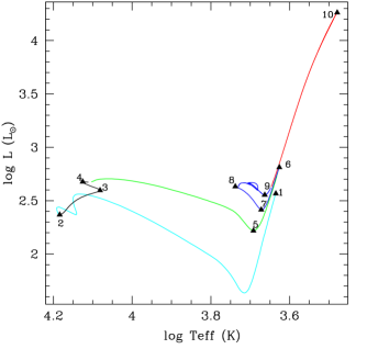
Figure 1: Evolution track in the Hertzsprung-Russell diagram of the standard 4.0 $M_{\odot}$  model at solar metallicity. Each phase is indicated by a different color : pre-main sequence (cyan), main sequence (black), Hertzsprung gap and red giant branch (green), core helium-burning phase (blue), and asymptotic giant branch (red). Black triangles show the points that we have selected to describe the tracks (see Sect.3.1)

We provide files containing sets of relevant physical quantities as a function of time that characterize our models computed in the initial mass range between 0.85 M_⊙  and 6.0 M_⊙  with four metallicities $Z=0.0001$, 0.002, 0.004 and 0.014 ([Fe/H]= -2.16, -0.86, -0.56, and 0 respectively). For each mass and metallicity, models are computed with standard prescriptions (no mixing other than convection process), and with both thermohaline instability and rotational transport. For all masses the evolution is followed from the beginning of the pre-main sequence (along the Hayashi track) up to the early-AGB phase. For each model, we have selected 500 points to allow a good description of the full raw tracks. First, key evolutionary points are determined (see Fig. 1):

1. beginning of the pre-main sequence;

2. ZAMS defined as the time when the central hydrogen abundance $X_{c}$ has decreased by 0.003 in mass fraction compared to its initial value.

3. turning point with the lowest $T_{\text{eff}}$ on the main sequence;

4. end of core H-burning defined as the point beyond which $X_{c}$ is smaller than $10^{-7}$ ;

5. bottom of the Red Giant Branch (RGB);

6. RGB-tip;

7. local minimum of luminosity during central He-burning;

8. local maximum of $T_{\text{eff}}$ during central He-burning;

9. bottom of AGB : point with local minimum of luminosity after the loop on HB ;

10. end of core He-burning defined as the point beyond which $Y_{c}$ is smaller than $10^{-4}$.

Table 2: Description of table containing result of our evolution models, both standard case and including rotation and thermohaline mixing.

Stellar parameters	Surface abundances	Central abundances
- Model number	1H 2H	1H
- Maximum of temperature $T_{\mathrm{max}}$ (K)	3He 4He	3He 4He
- Mass coordinate of $T_{\mathrm{max}}$ ($M_{\odot}$)	6Li 7Li
- Effective temperature Teff (K)	7Be 9Be
- Surface luminosity L (L⊙)	10B 11B
- Photospheric radius radius Reff (R⊙)	12C 13C 14C	12C 13C 14C
- Photospheric density $\rho_{eff}$ (g.$\mathrm{cm^{-3}}$)	14N 15N	14N
- Density at the location of $T_{max}$, $\rho_{max}$ (g.$\mathrm{cm^{-3}}$)	16O 17O 18O	16O 17O 18O
- Stellar mass M ($M_{\odot}$)	19F	19F
- Mass loss rate ($\mathrm{M_{\odot}.yr^{-1}}$)	20Ne 21Ne 22Ne	20Ne 21Ne 22Ne
- Age t (yr)	23Na	23Na
- Photospheric gravity $log(g_{\mathrm{eff}})$ (log(cgs))	24Mg 25Mg 26Mg	24Mg 25Mg 26Mg
- Central temperature $T_{c}$ (K)	26Al 27Al	26Al 27Al
- Central pressure $P_{c}$	28Si	28Si
- Surface velocity $v_{surf}$ ($\mathrm{km.s^{-1}}$)
- Mass at the base of convective envelope ($M_{\odot}$)
- The large separation from scaling relation $\Delta\nu_{\mathrm{scale}}$ ($\mathrm{\nu Hz}$)
- The large separation from asymptotic relation $\Delta\nu_{\mathrm{asymp}}$ ($\mathrm{\nu Hz}$)
- The frequency with the maximum amplitude $\nu_{\mathrm{max}}$
- The maximum amplitude $A_{\mathrm{max}}$
- The asymptotic period spacing of g-modes $\Delta\mathrm{\Pi}$ (s)
- The total acoustic radius T (s)
- The acoustic radius at the base of convective evelope tBCE (s)
- The acoustic radius at the location of helium second-ionisation region tHe (s)

The data in the tables are linearly interpolated within the results of each evolutionary model. We perform the interpolation as a function of time, central mass fraction of hydrogen or helium, or luminosity according to the evolutionary phase, and the final interpolated values are given at 499 points that we distribute as follows:

• 99 points evenly distributed in time sample the pre-main sequence between points 1 and 2.

• 110 points evenly distributed in terms of the central hydrogen mass fraction $X_{C}$ sample the main sequence with 85 points distributed between points 2 and 3, and 25 points distributed between points 3 and 4.

• 60 points evenly spaced in time sample the Herzsprung gap between points 4 and 5.

• 80 points evenly distributed in terms of $\log L$ sample the RGB between points 5 and 6.

• 20, 70 and 70 points evenly distributed in terms of $Y_{C}$ respectively sample the central He burning phase between points 6 and 7 , 7 and 8 and, 8 and 9.

• Finally, 50 points evenly spaced in $\log L$ are selected between points 9 and 10

For each model, we store the quantities given in table 2 in a file that can be retrieved from http://obswww.unige.ch/Recherche/evol/-Database- .

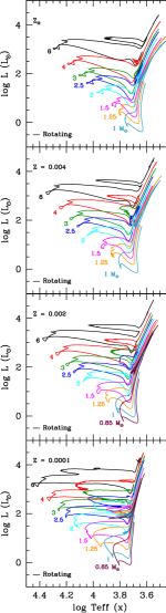
Figure 2: Theoretical evolution tracks in the HR diagram for the ensemble of calculated models for all metallicities ($Z_{\odot}$, Z=0.004, Z=0.002, and Z=0.0001, from top to bottom). On left panels the tracks are shown for the rotating models from the pre-main sequence on. On the right panels, both standard and rotating predictions are shown (dashed and solid lines respectively) from the ZAMS and beyond.

3.2 Comparisons between models from Ekström et al. (2012, Geneva code) and our models (STAREVOL)

Ekström et al. (2012) computed a large grid of models with rotation from 0.8 to 120 M_⊙ at solar metallicity with the Geneva stellar evolution code. The present grid is complementary since the low-mass star models of Ekström et al. (2012) are computed only to the helium flash at the RGB tip and do not include thermohaline mixing. Also, we presently explore asterosismic diagnostics during the TP-AGB.

In order to offer this complementarity between the 2 sets of giants, we were careful in choosing the same input physics and assumptions, although some differences remain that we describe below. Both codes use the same physical inputs for convection (Schwarzschild criterion and overshoot), opacities, mass loss, and nuclear reaction rates, and for the mass domain explored the different equations of state have a negligible impact on the stellar structures. Besides, the initial abundances of our models are similar apart from the larger number of species followed in STAREVOL. STAREVOL has indeed a more extended network of nuclear reactions than the Geneva code, which allows to follow in particular the evolution of unstable elements such as ${}^{13}N$, ${}^{15}O$, and ${}^{7}Be$. As a consequence, the convective cores are smaller on the main sequence in STAREVOL models (by $\sim$7% for the [4.0 M_⊙, Z_⊙] model), and the tracks in the HR-diagram are slightly less luminous ($L_{\text{TO}}$ is $\sim$10% lower for the [4.0 M_⊙, Z_⊙] model). This results in a difference in the lifetime on the main sequence 4% for the [4.0 M_⊙, Z_⊙] model. This is the main difference we could identify when comparing standard models computed with the two codes.

For the rotational transport both codes follow the advection by meridional circulation and the diffusion by shear turbulence. We carefully checked that the use of a different prescription for the turbulent diffusion coefficient $D_{v}$ (Talon & Zahn (1997) in STAREVOL and Maeder (1997) in Geneva code) has no impact in the mass domain we explore as the mixing above the convective core is dominated by $D_{\text{eff}}$. Both codes use prescriptions from Zahn (1992) for the horizontal diffusion coefficient, $D_{h}$. However in STAREVOL we always use Eq.7 that is given by Zahn (1992) to avoid the divergence of effective diffusion coefficient ($\propto$ $\frac{1}{D_{h}}$), while in Geneva the original Eq.2.29 of Zahn (1992) is used. Surprisingly Eq.7 implies higher values of $D_{h}$ at the edge of the convective core (by about a factor of 4 in the [4.0 M_⊙, Z_⊙] model on the main sequence), which leads to less mixing in these central regions. Combined with the fact that STAREVOL models have a lower initial rotation velocity on the zero age main sequence, this results in a lower lifetime and lower luminosity (the maximum difference being of 15% for the [4.0 M_⊙, Z_⊙] model).

4 Global properties of the models

The effects of rotation-induced mixing and thermohaline instability on the surface chemical properties of the grid stars were extensively discussed in Papers I and II. Here we focus on the global properties of the models

4.1 Hertzsprung-Russell diagrams and logTc vs log$\rho_{c}$

The evolutionary tracks in the HR diagram are shown in Fig.2 for all the models computed in this study, with and without rotation. We also present the evolution of the central temperature and density in Fig.3 for the solar-metallicity case.

4.1.1 Metallicity effects

Let us first recall the impact of metallicity as already reported in the literature (e.g. Schaller et al. 1992; Schaerer et al. 1993; Charbonnel 1994; Heger & Langer 2000; Maeder 2009). For a given stellar mass one notes the following effects when metallicity decreases, due to the lowering of the radiative opacity:

• The ZAMS is shifted to the blue, and both the stellar luminosity and effective temperature are higher at that phase compared to solar metalicity models.

• The positions of the RGB and of the AGB are shifted to the blue, and the ignition of helium (in degenerate conditions or not) occurs at lower luminosity at the tip of the RGB (L=21308 L_⊙ and 21252 L_⊙ for models [1.5M_⊙, Z=0.014 and Z=0.002] respectively).

• Central helium burning occurs at a higher effective temperature, and more extended blue loops are obtained.

4.1.2 Impact of rotation-induced mixing and thermohaline instability

• As known for a long time (see e.g. Maeder & Meynet 2000) and as shown in Fig.2, rotation-induced mixing affects the evolution tracks in HR diagram. On the main sequence, rotational mixing brings fresh hydrogen fuel into the longer lasting convective core, and transports H-burning products outwards. This results in more massive helium cores at the turnoff than in the standard case and shifts the tracks towards higher effective temperatures and luminosities all along the evolution (Ekström et al. 2012; Heger & Langer 2000; Maeder & Meynet 2000; Meynet & Maeder 2000). The right panel of Fig.3 shows the central conditions in standard and rotating models for selected masses at solar metallicity. Rotating models behave as star with higher mass during all of their evolution.

• Thermohaline mixing induced by ³He-burning becomes efficient only on the RGB at the bump luminosity (Charbonnel & Zahn 2007b; Charbonnel & Lagarde 2010). Beyond this point the double-diffusive instability develops in a very thin region located between the hydrogen-burning shell and the convective envelope, and has negligible effect on the stellar structure. It does not modify the evolution tracks in the HR diagram nor in the log T_c vs log $\rho_{C}$ diagram.

4.2 Lifetimes

The theoretical lifetimes are shown in Fig.4 for the main phases of evolution as a function of the initial stellar mass and for the four metallicities considered, with the effects of rotation being presented. Let us recall the main points:

• The duration of all the evolutionary phases decreases when the initial stellar mass increases and when the metallicity decreases (Schaller et al. 1992; Schaerer et al. 1993; Charbonnel 1994), which is consistent with the above-mentioned luminosity and effective-temperature differences.

• After the bump luminosity the thermohaline mixing does not affect the lifetimes on the RGB and on the early-AGB phases.

• The lifetimes of rotating models on the main sequence are increased compared to those of the standard models. Indeed rotation-induced mixing brings fresh hydrogen fuel in the stellar core during that phase. As a consequence, the exhaustion of hydrogen in the central region is delayed and the lifetime on the main sequence increases; additionally the mass of the He-core is larger at the end of main sequence when rotation is accounted for (Ekström et al. 2012; Heger & Langer 2000; Maeder & Meynet 2000; Meynet & Maeder 2000).

• As a consequence of having a more massive core at the end of the main sequence due to rotation, the models that undergo the He-Flash spend a shorter time on the RGB (see Fig. 4). Similarly to the MS, all rotating models have a longer lifetime during the quiescent central He burning phase.

• Lifetimes on the early-AGB are longer in rotating models than in standard models, due to their more massive core. This remains unchanged if we add the lifetime on the TP-AGB (1.1.10⁶ yr for [1.5 M_⊙, Z_⊙] and 2.10⁶ yr for [3 M_⊙, Z_⊙] ) to the early-AGB as the total lifetime on the AGB is only increased by a few percent.

• As seen in previous subsections thermohaline mixing has a negligible impact on the stellar structure, and does not modify the stellar evolutionary tracks. Similarly it does not impact on lifetimes.

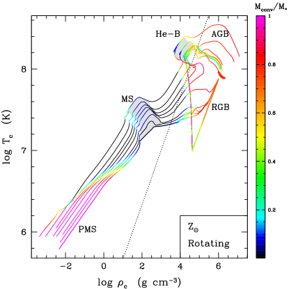
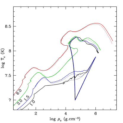
Figure 3: Left panel Central density as a function of central temperature for the rotating $Z_{\odot}$ models. Colours indicate the mass of convective regions (convective core and convective envelope) over the total stellar mass. Shaded regions indicate the phases of central hydrogen-burning (MS) and helium-burning (He-B). Right panel Central density as a function of central temperature for standard and rotating models (dashed and solid lines respectively) for four initial stellar masses from the ZAMS beyond.

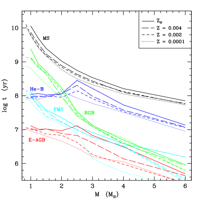
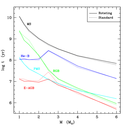
Figure 4: Duration of the different evolution phases as a function of the initial stellar mass. (left) Effects of metallicity for the standard models. (right) Effects of rotation at solar metallicity.

5 Global asteroseismic quantities

In recent years, a large number of asteroseismic observations have been obtained for different kinds of stars. In particular, the detection and characterization of solar-like oscillations in a large number of red giants by space missions (e.g. De Ridder et al. 2009) promises to add valuable and independent constraints to current stellar models. The confrontation between models including a detailed description of transport processes in stellar interiors and these asteroseismic constraints opens a new promising path for our understanding of stars.

Rotation is one of the key processes that change all outputs of stellar models (see Sect. 4) with a significant impact on asteroseismic observables. In the case of main-sequence solar-type stars, rotation is found to shift the evolutionary tracks to the blue part of the HR diagram resulting in higher values of the large frequency separation for rotating models than for non-rotating ones at a given evolutionary stage Eggenberger et al. (2010a). For red giants, rotating models are found to decrease the determined value of the stellar mass of a star located at a given luminosity in the HR diagram and to increase the value of its age. Consequently, the inclusion of rotation significantly changes the fundamental parameters determined for a star by performing an asteroseismic calibration Eggenberger et al. (2010b).

5.1 Scaling relations and asymptotic quantities provided for the present grid

Z=0.014 M=2.0 $M_{\odot}$  

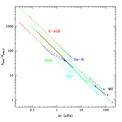
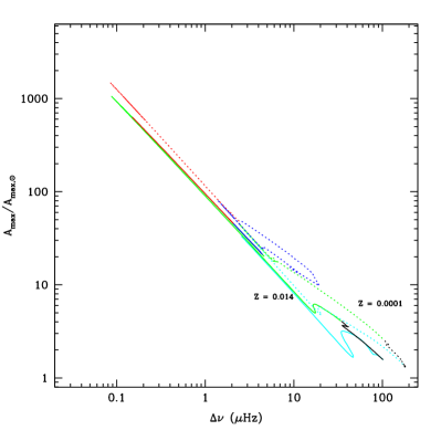
Figure 5: Maximal amplitude compared to solar as a function of the large separation: (left panel) at solar metallicity for 1.25 $M_{\odot}$, 2.0 $M_{\odot}$, and 6.0 $M_{\odot}$ rotating models, and (right panel ) at two metallicities Z=0.014 (solid lines) and Z=0.0001 (dotted-lines) for a 2.0 $M_{\odot}$  rotating model. Evolutionary phases are color-labeled: pre-main sequence (cyan), main sequence (black), RGB (green), He-burning (blue), and AGB (red)

For this new grid of standard and rotating models, we now provide the values of different asteroseismic parameters (see Table 2) that can be directly computed from global stellar properties using scaling relations. We also use the information on the internal structure of models to compute asymptotic relations. These scaling relations are particularly useful to constrain stellar parameters and to obtain new information about stellar evolution without the need to perform a full asteroseismic analysis (see e.g. Stello et al. 2009; Miglio et al. 2009; Hekker et al. 2009; Mosser et al. 2010; Chaplin et al. 2011b; Beck et al. 2011; Bedding et al. 2011). Although solar-like oscillations are expected to be excited in relatively cool stars (main-sequence as well as red giant stars), these global asteroseismic quantities are provided for all models of our grid and not only for models with a significant convective envelope.

The first global asteroseismic quantity we provide is the large frequency separation $\Delta\nu$, which is expected to be proportional to the square root of the mean stellar density (e.g. Ulrich 1986):

$$\Delta\nu_{\mathrm{scale}}=\Delta\nu_{\odot}\left(\frac{M}{M_{\odot}}\right)^{0.5}\left(\frac{R}{R_{\odot}}\right)^{-1.5},$$ (8)

with the solar large frequency separation $\Delta\nu_{\odot}=134.9\mathrm{\mu Hz}$.

Belkacem et al. (2011) have proven that the frequency $\nu_{\mathrm{max}}$ at which the oscillation modes reach their strongest amplitudes is approximatively proportional to the acoustic cut-off frequency, as suspected by Brown et al. (1991) and Kjeldsen & Bedding (1995).

$$\nu_{\mathrm{max}}=\nu_{\mathrm{max},\odot}\left(\frac{M}{M_{\odot}}\right)\left(\frac{R}{R_{\odot}}\right)^{-2}\left(\frac{T_{\mathrm{eff}}}{T_{\mathrm{eff,\odot}}}\right)^{-0.5},$$ (9)

with the solar value $\nu_{\mathrm{max,}\odot}=3150\mathrm{\mu Hz}$.

Finally, the value of maximum oscillation amplitude relative to that of the Sun ($A_{\mathrm{max}}/A_{\mathrm{max,}\odot}$) is computed using the following relation (e.g. Huber et al. 2011) :

$$A_{\mathrm{max}}/A_{\mathrm{max,}\odot}=\frac{(L/L_{\odot})^{s}}{(M/M_{\odot})^{t}}\left(\frac{T_{\mathrm{eff}}}{T_{\mathrm{eff,\odot}}}\right)^{-r},$$ (10)

with the solar value from Kepler $A_{max,\odot}=2.5\mathrm{ppm}$.
Following Huber and collaborators we adopt s=0.838 and t=1.32. A value of $r=2$ is adopted as advocated by Kjeldsen & Bedding (1995). Note that we simply assume that these relations hold for the different models computed here and we do not test the validity of the scaling relations. Preliminary studies suggest that these simple scaling relations hold reasonnably well for main sequence and RGB stars (e.g. Stello et al. 2009; White et al. 2011).
In addition to the asteroseismic observables deduced from scaling relations, asymptotic asteroseismic quantities are also provided.

The asymptotic large frequency separation is given by :

$$\Delta\nu_{\mathrm{asymp}}=\left(2\int_{0}^{R}\frac{dr}{c_{s}}\right)^{-1},$$ (11)

where R is the stellar radius, and c_s is the sound speed.

The total acoustic radius T is provided using the following relation, which is directly related to the large frequency separation :

$$T=\int_{0}^{R}\frac{dr}{c_{s}}=\frac{1}{2\cdot\Delta\nu_{\mathrm{asymp}}},$$ (12)

The acoustic radius at the base of convective envelope (t_BCE) and at the location of helium second-ionisation region (t_He) are determined with following relations :

$$t_{\mathrm{BCE}}=\int_{0}^{r_{\mathrm{BCE}}}\frac{dr}{c_{s}}\hfill,\hfill t_{\mathrm{He}}=\int_{0}^{r_{\mathrm{He}}}\frac{dr}{c_{s}},$$ (13)

where r_BCE and r_He represent the stellar radius at the base of convective envelope and at the location ofhelium second-ionization zone.

The period spacing of gravity modes for $\ell$=1 and different acoustic radii can be determined with the following asymptotic relation :

$$\Delta\mathrm{\Pi}(\ell=1)=\frac{2^{\frac{1}{2}}\cdot\pi^{2}}{\int_{r_{1}}^{r_{2}}N\cdot\frac{dr}{r}},$$ (14)

where N is the Brunt-Väisälä frequency. r₁ and r₂ define the domain (in radius) where the g modes are trapped. Within this region, the mode frequency ($\omega$) must satisfy the following conditions :

$$\omega^{2}<N^{2}$$ (15)

and

$$\omega^{2}<S_{\mathrm{l}}^{2}=\frac{l(l+1)c_{s}^{2}}{r^{2}}$$ (16)

with S_l the lamb frequency.

In the following discussions, we use the large separation determined with the scaling relation $\Delta\nu_{\rm scale}$(noted $\Delta\nu$ in the following sections). We have compared the large separation estimates $\Delta\nu_{\mathrm{scale}}$ (Eq. 8) and $\Delta\nu_{\mathrm{asymp}}$ (Eq. 11) to evaluate the difference between both expressions. On the main sequence, this difference varies between 3 and 5% for 1.0 M_⊙ model at solar metallicity. We find that the relative error obtained when using Eq. 8 or Eq. 11 depends on the stellar mass (i.e. 3-8% for [2.0 M_⊙, Z_⊙] MS model), the metallicity (i.e. 10-12% for the [2.0 M_⊙, Z=10^-4] MS model), and the evolutionnary phase (i.e. $<$15% on RGB, $<$10% on He-B both for [1.0 M_⊙, Z_⊙] model). A forthcoming work, out of the scope of the paper, is necessary to interpret these differences and to see how they compare to White et al. (2011)

5.2 Evolution of the asteroseismic observables

We now describe the global asteroseismic properties of low- and intermediate-mass stars along their evolution, and discuss the impacts of stellar mass, metallicity, and of non-standard mixing mechanisms. We illustrate our discussion with Fig. 5 to 10. In Fig.5 we present the maximal oscillation amplitude as a function of the large frequency separation all along the evolution from the pre-main sequence to the AGB phase for three different initial stellar masses at solar metallicity (left panel) and for a 2 $M_{\odot}$ star for the lowest (Z=0.0001) and the highest (Z=0.014) metallicities explored here (right panel). The line colors change with the stellar evolution phases: cyan corresponds to the pre-main sequence, black to the main sequence, green to the red giant branch, blue to core helium-burning, and red to the asymptotic giant branch. Fig. 6 presents the same quantities for all the stellar masses considered at solar metallicity, for both the standard and the rotating cases (dashed and solid lines respectively), each evolutionary phase being presented singly.

Pre-Main sequence Main Sequence  


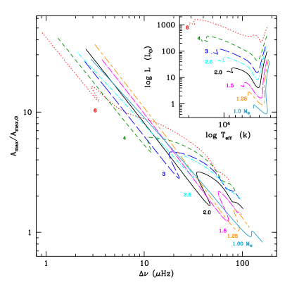
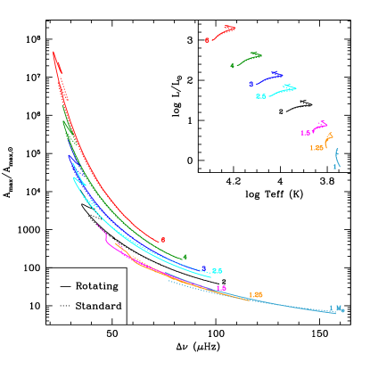
                                 Red Giant Branch                               He-Burning  

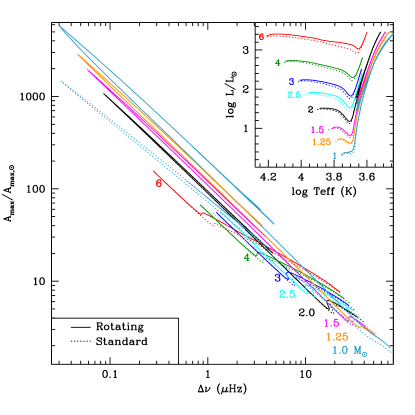
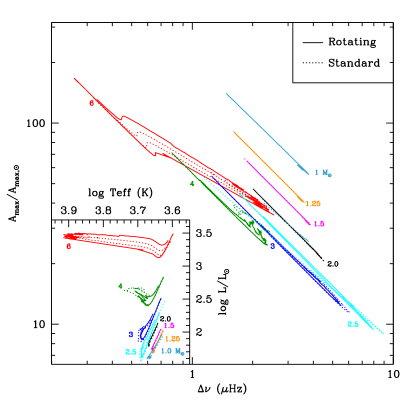
Figure 6: Maximal amplitude compared to solar as a function of the larger separation for models at $Z_{\odot}$. Top-left panel: on the pre-main sequence ; top-right panel: on the main sequence ; bottom-left panel: on the red giant branch ; bottom-right panel: on He-burning phase. Standard models and rotating models are shown with dashed and solid lines respectively except for pre-main sequence. The corresponding evolution in the Hertzsprung-Russell diagram is shown on the right corner of each panel

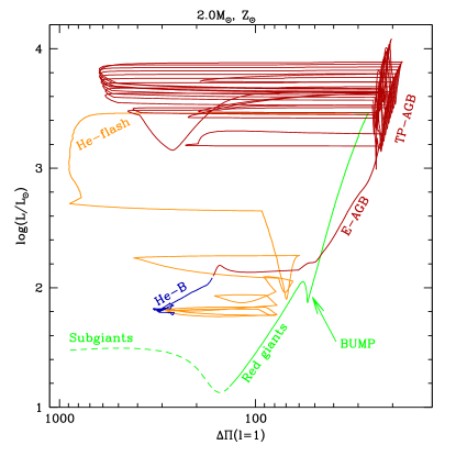
Figure 7: The stellar luminosity as a function of the asymptotic period spacing of g-modes for the standard 2.0 M_⊙ model at solar metallicity. Evolutionary phases are color-labeled: subgiant (green dashed), red giant (green solid), He-flash episod (orange), He-burning (blue), and asymptotic giant branch (red)

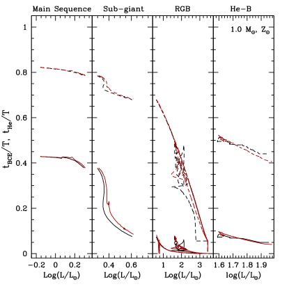
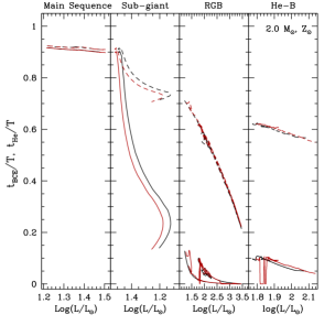
Figure 8: Acoustic radius at the base of the convective envelope (t_BCE, solid line) and at the base of He-ionization zone (t_He, dashed line) compared to total acoustic radius T as a function of the stellar luminosity for (left panel) 1.0 and (right panel) 2.0 M_⊙ models at solar metallicity following standard (black line) and rotating prescriptions (red line) ; (from left to right) on the main sequence, the sub-giant branch, red giant branch, and He-burning phase.

5.2.1 Trends for a given stellar mass and metallicity - the case of the 2.0 $M_{\odot}$,  $Z_{\odot}$models

In the following we describe the evolution of the seismic properties of a star of 2.0 $M_{\odot}$ at solar metallicity as depicted by the solid line in Fig.5 and the black line in Fig.6. Although this 2 M_⊙ star is not expected to show solar-like oscillations during the main sequence due to its too large surface temperature, it represents a typical model for a red giant exhibiting solar-like oscillations. Moreover, the discussion of the changes of the asteroseismic quantities during the main sequence remains globally valid for less massive main-sequence stars (the main difference being the value of the ratio between the acoustic radius at the base of the convective envelope and the total acoustic radius, see Fig. 8).

The large separation $\Delta\nu$ increases along the pre-main sequence because of its inverse dependence in stellar radius, which decreases during that phase (see Eq.14). On the other hand, the simultaneous decrease of maximal amplitude $A_{\mathrm{max}}/A_{\mathrm{max,}\odot}$ results from the decrease of luminosity and from the rise of effective temperature (see Eq.10).

On the main sequence, $A_{\mathrm{max}}/A_{\mathrm{max,}\odot}$ rises because of its dependence with luminosity and with the inverse of the effective temperature. In addition, the expansion of the stellar radius causes $\Delta\nu$ to increase. The radius increase also causes the large separation to drop significantly as the model evolves on the RGB, while the maximum amplitude increases during this phase as a result of the luminosity increase and the effective temperature decrease.

After the He-flash at the tip of the RGB, the luminosity and the stellar radius dwindle with a rise of effective temperature, implying that the maximum of amplitude wanes while the large separation increases. Throughout the helium burning phase, the luminosity and stellar radius increase while the effective temperature and stellar mass decrease. Consequently, a gain of $A_{\mathrm{max}}$ is obtained while the large separation reduces.

Figure 7 presents the asymptotic period spacing of gravity modes $\Delta\mathrm{\Pi}$($\ell$=1) for the standard model of 2.0 M_⊙ at solar metallicity. As proposed by Bedding et al. (2011) and Mosser et al. (2011), this quantity allows to distinguish two stars that have the same luminosity, one being at the RGB bump and the other one being at the clump undergoing central He burning. Indeed, at log(L/L_⊙) $\sim$ 2.0, $\Delta\Pi$($\ell$=1)=55 s at the RGB bump, and $\Delta\mathrm{\Pi}$($\ell$=1)=190 s in the clump. As the stellar structure, and more particularly the presence of the convective core affects the domain where the g-modes are trapped, $\Delta\mathrm{\Pi}$($\ell$=1) is larger in clump stars than in RGB stars (Christensen-Dalsgaard 2011). Large variations of $\Delta\mathrm{\Pi}$($\ell$=1) are observed during the thermal pulses and He-flash phase because of the formation of an intermediate convective zone during the He-flashes and thermal pulses. We consider that the modes are trapped in the outermost radiative zone leading to a large value of $\Delta\mathrm{\Pi}$($\ell$=1) (Bildsten et al. 2012).

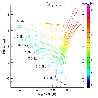
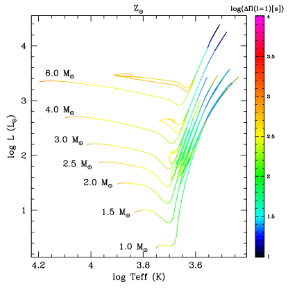
Figure 9: Color-coded HR diagram for all the masses in the grid at solar metallicity. The color code represents the values (in seconds) of the acoustic radius at the base of the ionization of He II $t_{\rm He}$ (left panel) and of the asymptotic period spacing of g-modes $\Delta\mathrm{\Pi}(\ell=1)$ (right panel). The values increase from blue to red in both cases as shown on the scales on the right of the plots.

Figure 8 shows the acoustic radius at the base of convective envelope (t_BCE) and at the base of He-ionization zone (t_He), both over the total acoustic radius as a function of luminosity, for the standard (black line) 1.0 M_⊙ (left panel) and 2.0 M_⊙ (right panel) models at solar metallicity from the main sequence to He-burning phase. As the extent (in radius) of the convective envelope decreases with increasing stellar mass on the main sequence, the difference between t_He and t_BCE becomes smaller.

As the convective envelope deepens inside the star with the first dredge-up, the acoustic radius t_BCE decreases during the subgiant branch. During this phase, the acoustic radius at the base of He II ionization zone follows the variation of effective temperature and t_He increases while T_eff decreases. In addition the total acoustic radius increases because of its dependence with the stellar radius that increases during this phase. Consequently, t_He/T decreases from 0.8 to 0.68 and from 0.9 to 0.7 for [1.0 M_⊙, Z_⊙] and [2.0 M_⊙, Z_⊙] models respectively . While the star ascends the RGB, t_BCE follows the convective envelope and the acoustic radius t_He/T decreases to 0.2 for 2.0 M_⊙ model until the RGB tip is reached (at log L/L${}_{\odot}\sim$ 3.5). When the stellar luminosity decreases after the RGB tip the convective envelope retracts in radius, and the effective temperature increases while the star contracts. Therefore t_BCE/T and t_He/T increase until the central temperature is sufficient to ignite helium. At the end of He burning phase, the surface layers expand and the convective envelope deepens while the effective temperature decreases. During this phase t_BCE/T and t_He/T in 2.0 M_⊙ model decrease slowly from $\sim$0.62 and $\sim$0.1 to $\sim$0.55 and $\sim$0.05 respectively.

Although we do not include this phase in the files presented in Sect.3.1, we discuss the evolution of the asteroseismic parameters during the TP-AGB. Figure 10 shows the evolution of stellar parameters ($L$,$T$_eff, and $M$), and asteroseismic parameters ($\Delta\nu$, $\nu_{\mathrm{max}}$, and $A_{\mathrm{max}}$) as a function of time from the first thermal pulse for 2.0 $M_{\odot}$  model at $Z_{\odot}$.

Between each thermal pulse, the stellar radius increases. The mass slowly decreases by steps at this phase, remaining almost constant during the inter-pulses. Then, the large separation decreases between each thermal pulse as well as $\nu_{\mathrm{max}}$ despite the slight decrease of effective temperature. The maximal amplitude increases as a result of the luminosity increase and the decrease of the effective temperature and total stellar mass. The strong increase of $A_{\mathrm{max}}$ during the interpulses is due to the large mass loss at this phase, better seen in the last pulse shown in Fig. 10.

5.2.2 Effects of metallicity

Although the current asteroseismic missions focus on solar metallicity stars, we present the effects of metallicity on the global asteroseismic parameters; they are depicted in Fig.5 (right panel) for a 2.0 $M_{\odot}$  model.

As discussed in 4.1.1, at lower metallicity the main sequence is shifted to the blue and to higher luminosity on HR diagram. Therefore, the track in the $A_{\mathrm{max}}$ vs $\Delta\nu$ plot is moved to lower $A_{\mathrm{max}}/A_{max,\odot}$ values. In addition, the luminosity of He-ignition at the RGB tip occurs at lower $A_{\mathrm{max}}/A_{max,\odot}$ when the metallicity is lower. The track all along the evolution in the $A_{\mathrm{max}}$ vs $\Delta\nu$ plot is shifted to the right (toward higher $\Delta\nu$ values) when the metallicity decreases. This is a direct consequence of a more metal-poor star behaving as a more massive star.

5.2.3 Effects of stellar mass

When the mass increases, the ZAMS (point at higher $\Delta\nu$ and lower $A_{\mathrm{max}}$) is shifted to lower $\Delta\nu$ and higher $A_{\mathrm{max}}$ (see Fig. 5 and top panels of Fig.6). Indeed, the large frequency separation at the point of ZAMS decreases because of its dependence with the mean stellar density. Similarly to the Hayashi tracks during the pre-main sequence, stars with different masses tend to join together in the $A_{\mathrm{max}}$ vs $\Delta\nu$ plot during the RGB and early-AGB phase (see green and red lines respectively in Fig. 5). When stellar mass increases stars follow more extended blue loops during the central He-burning phase. As shown in Fig. 6 (bottom right panel), blue loops range over high $\Delta\nu$ and low $A_{\mathrm{max}}$/A_max,⊙.

Figure 9 shows the theoretical evolution of the stellar acoustic radius at the base of He-ionization zone and of the asymptotic period spacing of g-modes along the evolutionary tracks in the HR diagram for models of different masses at solar metallicity. Both quantities variations are expressed in seconds. Evolution is shown from the pre-main sequence to the early-AGB phase and from the subgiant branch to the early-AGB phase for t_He and $\Delta\Pi$ respectively. At a given evolutionary phase, the larger the stellar mass, the larger also the acoustic radius at the base of He-ionization zone. The same is true for $\Delta\Pi$.

5.2.4 Impact of rotation on the evolution along the amplitude vs $\Delta\nu$ diagram

In this section, we focus on the effect of accounting for rotational mixing on the global asteroseismic parameters. As thermohaline mixing solely affects the abundance at the surface and at the external layers of HBS pattern during the giant phase, without modifying the temperature, radius, luminosity or mass of the models, this process has no impact on the global asteroseismic parameters. It is nevertheless not excluded that well chosen asteroseismic parameters might help constraining the thermohaline mixing.

As discussed in Sect. 4, rotation modifies the position of the evolution tracks in the HR diagram (see Fig. 2). Consequently, differences appear on the maximal amplitude and the large separation, between standard and rotating models. This effect clearly shows up at the end of the main sequence due to the increased width of the main sequence in rotating models.
Then on the subgiant branch rotating models evolve at higher luminosities than their standard counterparts, which implies higher maximal amplitude. Rotation has no impact on the ratios t_BCE/T and t_He/T as seen in Fig. 8. In this figure, the effect of rotation on the stellar luminosity during the subgiant phase is also shown.
When the stars reach the RGB, the differences in effective temperature and luminosity between standard and rotating models become marginal; therefore the tracks are almost identical in the Figure 6 (bottom left panel).
Rotation affects the extension and width of the blue loops. As a consequence, the differences in asteroseismic parameters appear during the combustion phase of He, as illustrated in Fig. 6 (bottom right panel).

Figure 10: From top to bottom: Evolution of global stellar properties (luminosity L, effective temperature T_eff and total stellar mass M) and asteroseismic parameters ($\Delta\nu$, and $\nu_{\mathrm{max}}$,A_max/A_max,⊙) on the TP-AGB of the [2.0 M_⊙, Z_⊙] model computed with rotation up to the RGB tip and thermohaline mixing all along the evolution. The abscissa is the time since the first thermal pulse.

5.3 Same point on HR-diagram, same asteroseismic parameters ?

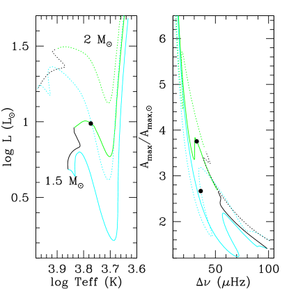
Figure 11: Left panel : Evolution tracks in Hertzsprung-Russel diagram of 1.5 and 2.0 $Z_{\odot}$(solid and dotted lines respectively) stars at solar metallicity. Right panel : Maximal amplitude over sun value as a function of the large separation for the same models. As in figure 5, the lines color indicates the evolutionary phase

Figure 11 shows how asteroseismic parameters can help to distinguish two stars with the same effective temperature and luminosity. On the left panel we show the 1.5 $M_{\odot}$ and 2.0 $M_{\odot}$ tracks in the HR diagram with the intersection indicated by the black dot. At this point, the 1.5 $M_{\odot}$ star is evolving on the HR gap and has the same effective temperature and luminosity as the 2.0 $M_{\odot}$ star evolving on the pre-main sequence. This black dot corresponds to two different points in the $A_{\mathrm{max}}$ vs $\Delta\nu$ plot shown on the right panel. As we can see, the larger separation of the 1.5 $M_{\odot}$  model is lower that of the 2.0 $M_{\odot}$, while the maximal amplitude is higher. These stars do not have the same mean stellar density, and therefore the same $\Delta\nu$. On the other hand, the total stellar mass is different at this point, and hence the maximal amplitude.

6 Conclusions

In this study we present a grid of single star evolution models in the mass range between 0.85 $M_{\odot}$  and 6.0 $M_{\odot}$, for four metallicities, including the impact of rotation and thermohaline mixing, along with standard models. All data detailed in Table 2 are available on the website http://obswww.unige.ch/Recherche/evol/-Database- for all the models computed (i.e., standard on one hand, and with rotation-induced mixing and thermohaline instability on the other hand) .

We recall the various impacts of metallicity variations and rotation-induced mixing on the stellar properties that were already discussed in literature. Thermohaline mixing does not change the stellar parameters like luminosity and effective temperature. As such this process does not affect the seismic properties as analyzed here. However and as discussed in Paper I and II, it changes the surface abundances from the bump luminosity on, and has to be taken into account to explain the observed chemical properties of bright giant stars.

Last but not least we also present the evolution of global asteroseismic parameters for all the models in our grid. The large frequency separation $\Delta\nu$, the frequency $\nu_{\mathrm{max}}$, and the maximum oscillation amplitude $A_{\mathrm{max}}$, are computed using scaling relations. Asymptotic asteroseismic quantities are also computed : $\Delta\nu_{\rm asympt}$, another estimate or the large frequency separation; $t_{\rm BCE}$, the acoustic radius at the base of convective envelope; $t_{\rm He}$, the acoustic radius at the base of the HeII ionization zone ; $T$, the total acoustic radius; and $\Delta\mathrm{\Pi}$($\ell$=1) , the period spacing of gravity modes.

We show that rotation-induced mixing has an impact on these quantities, contrary to thermohaline mixing. While rotation changes the global properties of main sequence stars and has an impact on the global asteroseismic properties, thermohaline mixing is negligible on these aspects although it changes the surface abundances in the red giants. In addition to spectrophotometric studies, seismic studies allow to distinguish two stars with approximatively the same luminosity and effective temperature but with different evolutionary stages.