Magnetic buoyancy instabilities in the presence of magnetic flux pumping at the base of the solar convection zone

Abstract

We perform idealised numerical simulations of magnetic buoyancy instabilities in three dimensions, solving the equations of compressible magnetohydrodynamics in a model of the solar tachocline. In particular, we study the effects of including a highly simplified model of magnetic flux pumping in an upper layer (“the convection zone”) on magnetic buoyancy instabilities in a lower layer (“the upper parts of the radiative interior – including the tachocline”), to study these competing flux transport mechanisms at the base of the convection zone. The results of the inclusion of this effect in numerical simulations of the buoyancy instability of both a preconceived magnetic slab and of a shear-generated magnetic layer are presented. In the former, we find that if we are in the regime that the downward pumping velocity is comparable with the Alfvén speed of the magnetic layer, magnetic flux pumping is able to hold back the bulk of the magnetic field, with only small pockets of strong field able to rise into the upper layer.

In simulations in which the magnetic layer is generated by shear, we find that the shear velocity is not necessarily required to exceed that of the pumping (therefore the kinetic energy of the shear is not required to exceed that of the overlying convection), for strong localised pockets of magnetic field to be produced which can rise into the upper layer. This is because magnetic flux pumping acts to store the field below the interface, allowing it to be amplified both by the shear, and by vortical fluid motions, until pockets of field can achieve sufficient strength to rise into the upper layer. In addition, we find that the interface between the two layers is a natural location for the production of strong vertical gradients in the magnetic field. If these gradients are sufficiently strong to allow the development of magnetic buoyancy instabilities, strong shear is not necessarily required to drive them (c.f. previous work by Vasil & Brummell). We find that the addition of magnetic flux pumping appears to be able to assist shear-driven magnetic buoyancy in producing strong flux concentrations that can rise up into the convection zone from the radiative interior.

1 Introduction

The Sun is observed to possess a large-scale predominantly toroidal field at the surface, which exhibits cyclic magnetic activity, as manifested by the sunspot cycle. Since the period of these cycles (approximately $11$ yr) is much shorter than the ohmic diffusion time for a primordial solar magnetic field ($10$ Gyr), it seems inescapable that we require the action of a dynamo which can generate magnetic fields to explain this behaviour. Since dynamos are generally assisted by differential rotation, it is believed that the tachocline, a region of strong radial (and somewhat weaker latitudinal) shear at the base of the convection zone of the Sun, plays an important role in this process, by generating toroidal field from poloidal field (Tobias & Weiss, 2007). The bulk of the solar toroidal field is likely to be stored just below the convection zone, both because the action of convective turbulence has been found to rapidly pump magnetic field into the nonturbulent regions beneath (e.g. Spiegel & Weiss 1980; Tobias et al. 2001), and also because the short rise time of buoyant magnetic flux tubes would pose problems for the storage of toroidal field at any depth in the convection zone (Parker, 1975).

Sunspots and other intense flux elements comprising active regions on the solar surface are thought to be produced by the instability of this large-scale toroidal field stored beneath the convection zone. A prime candidate for the instability mechanism is magnetic buoyancy. This can be explained in brief as the idea that a horizontal magnetic field $\mathbf{B}$ can support heavy gas above by virtue of the pressure ($|\mathbf{B}|^{2}/2\mu_{o}$) that it exerts. If it is in thermal equilibrium, the gas in the region of the field will therefore rise, since it is lighter than its surroundings. A horizontal magnetic field that decreases with height can render the fluid top-heavy, which is liable to instability.

Previous work has studied the instability of a field that decreases smoothly with height, in which case the unstable modes can be either two-dimensional “interchange modes” or three-dimensional “undular modes”, of which the latter are usually dominant (see, for example, the following review articles: Hughes & Proctor 1988; Hughes 2007). If the field is discontinuous and consists of a slab of horizontal magnetic field sandwiched by nonmagnetic gas in a convectively stable atmosphere, then the instability is of Rayleigh-Taylor type, and occurs for any strength of magnetic field (in the absence of diffusion). In this case the instability is a two-dimensional interchange mode, which involves no bending of the field lines (Cattaneo & Hughes, 1988). However, the nonlinear evolution of the instability can generate three-dimensional arched structures that qualitatively resemble those observed at the surface. These arise through the interactions between vortices, which are primarily generated by Kelvin-Helmholtz instabilities (vorticity is also produced by baroclinicity, a linear effect associated with the initial instability) driven by the rising magnetic “mushrooms” (Matthews, Hughes & Proctor 1995; Wissink et al. 2000). An important question concerns the scales of the rising magnetic structures. In the absence of diffusion the instability occurs at very small scales, and it is hard to see how such modes can lead to the large coherent structures seen at the surface. Larger length scales can be obtained either by using enhanced turbulent diffusion (and numerical computations are inevitably diffusive and show the same effect), or as a result of helicity in the magnetic field structures, for example through rotation.

In reality, the predominant source of the solar toroidal field is likely to be the strong radial (and somewhat weaker latitudinal) shear in the tachocline. This effect results from the variation in the angular velocity in the solar interior, which can stretch any poloidal field to produce toroidal field. While any poloidal field is unlikely to be coherent in the tachocline, it is certainly likely to be present to some degree. Recent work has therefore begun to address the problem of the generation of a toroidal magnetic layer through shear, together with the resulting magnetic buoyancy instabilities of this layer (e.g. Brummell et al. 2002; Cline et al. 2003; Vasil & Brummell 2008, hereafter VB08; Vasil & Brummell 2009, hereafter VB09; Silvers, Vasil, Brummell & Proctor 2009; Silvers, Bushby & Proctor 2009, hereafter SBP09).

Of most relevance to this work, VB08 and SBP09 used numerical simulations in Cartesian geometry to study the generation and subsequent instability of a horizontal magnetic layer from an initially uniform vertical field. They found that strong velocity shear, which is hydrodynamically unstable to Kelvin-Helmholtz type shear instabilities, is required for magnetic gradients to be sufficient for magnetic buoyancy instabilities to develop. Since the shear in the tachocline is believed to be much weaker, and hydrodynamically stable, this result appeared to provide a problem for the efficacy of this mechanism in producing buoyant flux structures. However, it is known that radiative diffusion (with diffusivity $\kappa$) below the convection zone is much more efficient at transporting heat than ohmic diffusion (with diffusivity $\eta$) is at transporting magnetic flux. In the regime that $\kappa\gg\eta$, it has long been known that double-diffusive effects could allow magnetic buoyancy instabilities (Gilman 1970; Acheson 1979; Schmitt & Rosner 1983) by mitigating the stabilising stratification through the action of radiative diffusion. It is therefore possible that a hydrodynamically stable tachocline shear can produce a magnetic layer that is unstable to a double-diffusive magnetic buoyancy instability. This was first confirmed by the simulations of Silvers, Vasil, Brummell & Proctor (2009), who used a similar setup to VB08, except in a parameter regime which favoured double-diffusive instabilities (see also Silvers et al. 2010). They showed that magnetic buoyancy instabilities of a shear-generated magnetic layer are possible in the double-diffusive regime, which is relevant for the Sun. In this paper we use the simplest model in which to investigate magnetic buoyancy instabilities, and do not study double diffusive effects, while recognising that a more complicated model should be considered in due course.

Whatever the mechanism by which these structures are produced, they then rise into the solar convection zone. The earlier calculations on shear-induced buoyancy did not in general include the action of the turbulent convection in this region. It is likely that the convection zone plays a crucial role in the solar dynamo process by helping to return flux of an appropriate orientation to the shear region so that the dynamo cycle can be completed. The effect of anisotropic and inhomogeneous turbulence on flux transport has been known for some time (Drobyshevski & Yuferev 1974; Arter et al. 1982; Arter 1983; Galloway & Proctor 1983; Tao et al. 1998). The principal effect is to transport horizontal magnetic flux down the gradient of turbulent intensity (Zeldovich 1957; Moffatt 1983). In the presence of a stable layer beneath, which is absent in convective turbulence, magnetic flux can be transported and stored in this layer (Tobias et al. 1998; Tobias et al. 2001; Dorch & Nordlund 2001; Ossendrijver et al. 2002; Kitchatinov & Rüdiger 2008). Numerical simulations of turbulent penetrative compressible convection show that magnetic flux is rapidly transported into the underlying stable layer on a convective (and not a diffusive) timescale by strong downflowing plumes (Tobias et al. 1998; Tobias et al. 2001; Dorch & Nordlund 2001), and that only the strongest field is able to counteract this effect and rise into the upper unstable layer. This phenomenon is robust and its physical basis is straightforward: in a stratified compressible convecting fluid there is a sharp distinction between rapidly falling and gently rising plumes (Weiss et al., 2004).

The purpose of this paper is to carry out a pilot study of the effects of the turbulent pumping on the evolution of the buoyancy instability. The computations referred to above show clearly that such an interaction is meaningful, with flux being transported not only on the smallest scales of the convection but on much larger scales too, so that there is a ‘mean’ effect. Ideally we would wish to study the interaction of magnetic buoyancy instabilities with the overlying convective flows in a direct numerical simulation, such as an extension of those presented in SBP09. However this is computationally challenging at the present time. Furthermore, we wish to understand the basic physics of the interaction of the atmosphere and the growing instabilities, without getting distracted by the complexities of the actual convection. Thus we choose to begin by constructing a model problem that captures the effect of the turbulence on the largest scales of the buoyancy modes by means of a mean-field ansatz. Clearly this simplification does not allow consideration of the largest scales of motion which are comparable or larger than the important buoyancy modes. Nor does it properly treat the small scales of the buoyancy which may be comparable with or smaller than those of the convection. Nonetheless the simple ansatz used does in our view capture important elements of the interaction, and gives a useful guide to more detailed calculations in the future. Note that our approach will not be strictly accurate at the base of the convection zone, where convection exists on a wide range of scales (e.g. Miesch et al. 2008). Averaging over the largest convection cells would then be meaningful only for the largest scales of the buoyant magnetic field. However, these models are not designed to accurately simulate the conditions at the base of the convection zone of the Sun. Instead, they are designed to provide a simple phenomenological picture of the magnetic pumping of large-scale fields resulting from small-scale convection, which can hopefully provide a complementary perspective to simulating the convection directly.

In keeping with the philosophy of modelling processes at the simplest non trivial level, we represent the magnetic pumping via mean-field electrodynamics as the antisymmetric part of the $\alpha$-tensor (e.g. Rädler 1968; Moffatt 1983), i.e., $\alpha_{ij}=\alpha\delta_{ij}-\epsilon_{ijk}\gamma_{k}$. This contributes an additional advective velocity to the induction equation for the mean magnetic field through the term $\nabla\times\left(\boldsymbol{\gamma}\times\mathbf{B}\right)$, where $\boldsymbol{\gamma}$ is a turbulent pumping velocity, which arises from a gradient in the turbulent intensity of the flow.

In this paper, we therefore study the effects of this mechanism on magnetic buoyancy instabilities by implementing a $\gamma$-pumping effect in numerical simulations of standard magnetic buoyancy.

We first extend previous calculations of the buoyancy instability of a preconceived magnetic slab (Cattaneo & Hughes 1988; Matthews, Hughes & Proctor 1995) by including the additional effect of magnetic pumping in an upper layer (“the convection zone”). This is designed to crudely mimic the addition of one of the most important effects of the convection zone on the nonlinear evolution of magnetic buoyancy instabilities of this magnetic slab. Though this is a very simple model, it is worthwhile to extend previous simulations through the addition of only this effect, to study in detail its influence on the problem. Later on, we extend previous calculations in which this magnetic layer is generated through shear acting on a vertical field, by including magnetic pumping in an upper layer. This should allow us to isolate the most important effect of an overlying convection zone on the nonlinear outcome of these instabilities.

The structure of the paper is as follows. We first describe the numerical setup of our simulations starting with a preconceived magnetic slab in §2. In this section we also discuss the simple model of magnetic pumping that we adopt. We then present the results of these simulations in §3. The numerical setup for the problem with shear is described in §4, and the corresponding results in §5. Finally, in §6 we present a discussion of the results and a summary of those which we deem to be important.

2 Numerical Model (without shear)

We adopt a Cartesian box with coordinates $(x,y,z)$, which represents a plane section of the tachocline region of the Sun. The entire domain extends from $z=0$ (top) to $z=d$ (bottom) in the vertical, and extends from $x,y=0$ to $x,y=\lambda_{x,y}d$ in the horizontal, where $\lambda_{x,y}$ will be specified later. We identify $xz$ as the poloidal plane (where $-\mathbf{e}_{z}$ is considered to be the radial direction), and $y$ as the toroidal (azimuthal) coordinate. An infinite slab of uniform toroidal magnetic field $\mathbf{B}=B_{0}\mathbf{e}_{y}$ is placed in the region $z\in[z_{1},z_{2}]$, which is sandwiched by nonmagnetic gas. The initial state is static, with a linear temperature distribution $T=T_{0}\left(1+\theta z/d\right)$, and is piecewise polytropic (with index $m$), being computed under the assumption that the total (gas plus magnetic) pressure is continuous at each magnetic interface. This is an unstable equilibrium configuration. If a small perturbation is imposed on the system, the density discontinuity at $z=z_{1}$ is unstable to a Rayleigh-Taylor type instability, which we excite by adding small random thermal perturbations to the top of the magnetic layer.

We assume the fluid is a perfect gas with constant shear viscosity $\mu$, thermal conductivity $\kappa$, magnetic diffusivity $\eta$ and specific heats $c_{p}$ and $c_{v}$ (which define the gas constant $\mathcal{R}=c_{p}-c_{v}$). The standard equations of mass, momentum, entropy and magnetic induction, together with the equation of state, can be non-dimensionalised by scaling lengths with the depth of the layer $d$, temperatures with the initial temperature at the upper surface $T_{0}$, densities with the initial density at the upper surface $\rho_{0}$, and magnetic fields with the magnitude of the initial magnetic field $B_{0}$ (e.g. Matthews, Proctor & Weiss 1995). We also use $d/\sqrt{\mathcal{R}T_{0}}$ as the unit of time, which corresponds to the sound travel time, using the isothermal sound speed at the top of the layer. Using this non-dimensionalisation, equations governing the temporal evolution of the density $\rho$, velocity $\mathbf{u}$, temperature $T$ and magnetic field $\mathbf{B}$ read

$$\partial_{t}\rho+\nabla\cdot\left(\rho\mathbf{u}\right)=0$$ (1)

$$\partial_{t}\left(\rho\mathbf{u}\right) = -\nabla\left(p+\frac{F}{2}|\mathbf{B}|^{2}\right)+\nabla\cdot\left(F\mathbf{B}\mathbf{B}-\rho\mathbf{u}\mathbf{u}+\sigma C_{K}\boldsymbol{\mathrm{\tau}}\right)$$ (2)

$$+\theta(m+1)\rho\mathbf{e}_{z}$$

$$\partial_{t}T = -\mathbf{u}\cdot\nabla T-(\gamma-1)T\nabla\cdot\mathbf{u}+\frac{\gamma C_{K}}{\rho}\nabla^{2}T$$ (3)

$$+\frac{C_{K}(\gamma-1)}{\rho}\left(\frac{\sigma}{2}||\boldsymbol{\mathrm{\tau}}||^{2}+F\zeta_{0}|\mathbf{J}|^{2}\right)$$

$$\partial_{t}\mathbf{B}=\nabla\times\left[\mathbf{u}\times\mathbf{B}-\zeta_{0}C_{K}\mathbf{J}\right]+\mathbf{G}$$ (4)

$$\nabla\cdot\mathbf{B}=0,$$ (5)

where the current $\mathbf{J}=\nabla\times\mathbf{B}$, the equation of state is $p=\rho T$, and the viscous stress tensor is

$$\tau_{ij}=\partial_{j}u_{i}+\partial_{i}u_{j}-\frac{2}{3}\delta_{ij}\partial_{k}u_{k},$$ (6)

and $\mathbf{G}$ will be specified later.

These equations contain seven dimensionless parameters, which, together with the initial and boundary conditions, completely determine the evolution of the system. These are the polytropic index $m$, the temperature gradient $\theta$, and the ratio of specific heats $\gamma=c_{p}/c_{v}$, together with the Prandtl number

$$\sigma=\frac{\mu c_{p}}{\kappa},$$ (7)

the ratio of magnetic to thermal diffusivity at the top of the layer

$$\zeta=\frac{\eta\rho_{0}c_{p}}{\kappa},$$ (8)

the dimensionless thermal diffusivity

$$C_{K}=\frac{\kappa}{\rho_{0}c_{p}d\sqrt{\mathcal{R}T_{0}}},$$ (9)

and the dimensionless field strengh

$$F=\frac{B_{0}^{2}}{\mathcal{R}T_{0}\rho_{0}\mu_{0}}.$$ (10)

The last quantity is related to the plasma $\beta$, which is the ratio of gas to magnetic pressure, by $F=2/\beta$. Note that the number of pressure scale heights in the domain is given by $N_{p}=(m+1)\ln(1+\theta)$. We always take $\gamma=\frac{5}{3}$, as is appropriate for a monatomic ideal gas, and will from now on reuse the symbol $\gamma$ to represent magnetic flux pumping, which we will define in § 2.1.

Eqs. 1–5 are solved subject to the boundary conditions that

$$u_{z}=\partial_{z}u_{x}=\partial_{z}u_{y}=0\;\;\;\;\;\;\;\;\;\;\;\;\mathrm{at}\;\;\;z=0,1,$$ (11)

$$T=1\;\;\;\mathrm{at}\;\;\;z=0,\;\;\;\partial_{z}T=\theta\;\;\;\mathrm{at}\;\;\;z=1.$$ (12)

These conditions represent impermeable, stress-free boundaries at the top and bottom of the computational domain. All horizontal (magnetic and nonmagnetic) boundary conditions are periodic. The mass flux and mechanical energy flux thus vanish on the boundaries, and the imposed heat flux is the only flux of (non-magnetic) energy into and out of the system. The vertical magnetic boundary conditions are

$$B_{x}=B_{y}=0\;\;\;\mathrm{at}\;\;\;z=0,1.$$ (13)

The field is therefore ensured to be vertical at the top and bottom boundaries. Note that any imposed horizontal field can leave the domain, since a gradient of these fields can exist at the boundaries. This choice of boundary conditions is somewhat artificial. However, the dynamics in the region not close to the vertical boundaries should only be weakly influenced by them.

The numerical method used to solve the above system of equations is a parallel hybrid finite-difference/pseudospectral code, where spatial derivatives are calculated in Fourier space for the horizontal directions and fourth-order finite-differences in the vertical direction (upwind derivatives being used for the advection terms). Time integration is performed by an explicit third-order Adams-Bashforth method. The equations solved, and the numerical method used are discussed in more detail in Matthews, Proctor & Weiss (1995) and Bushby & Houghton (2005), for example. The code has been thoroughly tested, particularly on problems of magnetoconvection and magnetic buoyancy.

We simulate a box that is elongated in the direction of the initial field, by choosing $\lambda_{x}=1$ and $\lambda_{y}=4$, so that the vortex tube instability observed by Matthews, Hughes & Proctor (1995) is allowed to develop and produce three-dimensional structure. We use a spatial resolution of $128\times 128\times 200$, except where specified otherwise.

2.1 Downward magnetic pumping

We add the following term into Eq. 4 to represent the effects of turbulent pumping of the magnetic flux from the upper “convective” regions, of the form

$$\mathbf{G}=\nabla\times\left(\boldsymbol{\gamma}\times\mathbf{B}\right),$$ (14)

with

$$\boldsymbol{\gamma}=\frac{\gamma_{m}}{2}\left[1+\tanh\left[(\Delta z_{i})^{-1}\left(z_{i}-z\right)\right]\right]\mathbf{e}_{z}.$$ (15)

The vertical profile is designed to represent a region with a uniform nonzero value (“the convection zone”) that smoothly goes to zero (“the radiation zone”) below a depth $z_{i}$ (“the radiative-convective interface”). We plot an example of such a profile in Fig. 1, using a set of typical values for the various parameters. This is a purely downward pumping velocity, which should act to prevent magnetic field with horizontal strengths smaller than

$$|\mathbf{B}_{h}|=B_{eq}\equiv\gamma_{m}\sqrt{\frac{\rho(z_{i})}{F}},$$ (16)

from rising into the upper layer. The evolution of the system after the onset of buoyancy instabilities will therefore depend on the parameter (noting that we initially take $B_{y}=1$)

$$M_{\gamma}=\gamma_{m}\sqrt{\frac{\rho(z_{i})}{F}}=\frac{B_{eq}}{B_{y}},$$ (17)

which is an Alfvénic Mach number for the $\gamma$-pumping. If $M_{\gamma}\lesssim 1$, we would expect some of the rising field to be able to overcome the downward pumping and rise into the upper layer. Alternatively, if $M_{\gamma}\gtrsim 1$, we would expect the field to be too weak to overcome the downward pumping, and $\gamma$ should therefore act as a lid which will hold down the field, unless the field can be locally amplified sufficiently that $|\mathbf{B}_{h}|>B_{eq}$.

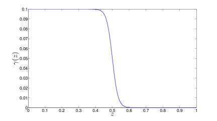
Figure 1: Typical profile of magnetic pumping with $z_{i}=0.5,(\Delta z_{i})^{-1}=30$ and $\gamma_{m}=0.1$.

The interpretation that we will adopt is that the Cartesian box represents a large horizontal section at the base of the convection zone. In this case, the spatial scale of the convection cells is considered to be much smaller than the horizontal size of the box. We can then reasonably assume a separation of scales and define an average over the small-scale convection cells. Our vertical scale is such that the upper layer ($z<z_{i}$) represents a significant fraction of the lower half of the convection zone, and $\gamma$ can be considered a “mean-field” pumping effect. In this interpretation, the simulated magnetic field, $\mathbf{B}$, is always considered to be a “mean field”, with the horizontal length scales of the magnetic field being much larger than that of the (unresolved) convection. It is then reasonable to consider $\gamma$ to act with equal strength on all of the resolved horizontal scales of $\mathbf{B}$ in our simulation, to a first approximation. For numerical reasons, it is essential to include nonzero diffusivities of momentum, heat and magnetic field. This means that the resolved diffusive lengthscales in the simulation are, by construction, larger than the horizontal scales of the unresolved small-scale convection. We consider the actual diffusive lengthscales to be much smaller than those of the unresolved convection. If desired, the simulated diffusivities can be considered to represent turbulent diffusivities resulting from the unresolved convection. However, we only include them for numerical reasons (though we will later include their effects in our discussion, for completeness), since we do not set out to study the effect of turbulent diffusivities on magnetic buoyancy.

Convective turbulence is also likely to pump the scalar fields of density and temperature, in addition to the magnetic field. If the turbulence is incompressible and only varies in one direction, such scalar pumping vanishes (leaving only anisotropic diffusion) because the pumping velocity is divergence-free (Moffatt, 1983), and when it exists it is, in general, not simply related to the velocity of magnetic pumping (Cattaneo et al., 1988). For compressible turbulence, it can be shown that an additional mean advection term arises (e.g. Vergassola & Avellaneda 1997), which may not necessarily vanish when the intensity of the turbulence varies only with height, as in our case. However, for simplicity, and since this effect is not simply related to $\gamma$, we choose to neglect pumping of scalar fields throughout this paper.

2.2 Parameters adopted

Convective flows in the lower parts of the convection zone are likely to be highly subsonic, with mach numbers inferred to be in the range $10^{-4}-10^{-2}$ (e.g. Ossendrijver 2003; Jones et al. 2010). In the simulations of Tobias et al. (2001), the magnetic pumping effect resulting from turbulent compressible convection occurs on a convective timescale. We might therefore expect $\gamma$ to be subsonic, with velocities at most comparable to the convective flows, constraining $\gamma_{m}\ll 1$.

In the tachocline, $\beta\sim 10^{7}$ (e.g. Tobias & Hughes 2004), which constrains $F\ll 1$. We must choose a much smaller $\beta$ for these calculations than in reality to speed up the initial instability. This is because the fastest growing Rayleigh-Taylor type mode has a growth rate which scales with $\beta^{-1}$ (Cattaneo & Hughes, 1988). We wish to study the nonlinear evolution of the instability in the presence of $\gamma$-pumping in the upper layer for a range of values of $M_{\gamma}$ either side of unity. To do this we fix a value of $F=0.01$ and vary $\gamma_{m}$. This fixes the growth rate and horizontal wavenumber of the initial instability, so that we can better isolate the consequences of varying the strength of the downward pumping. The parameter values adopted for these simulations are summarised in Table 1.

At the base of the convection zone the diffusivities are ordered such that $1\gg\kappa\gg\eta\gg\nu$ (Gough 2007; Jones et al. 2010). We respect this ordering by choosing $1\gg\zeta_{0}\gg\sigma$ and $C_{K}\ll 1$, though we do take much larger diffusivities than are present in the Sun, as is required if we are to run fully resolved simulations with a sensible run time. The stratification that we adopt has approximately three pressure scale heights within the domain. This is designed to roughly correspond with a region straddling the base of the convection zone (Christensen-Dalsgaard & Thompson, 2007). Note, however, that the upper layer in which $\gamma$-pumping is present also has subadiabatic stratification (since we fix $m>1/(1-\gamma)=3/2$), unlike in the convection zone of the Sun. We have also performed simulations in which the initial stratification changes from adiabatic to subadiabatic when $z>0.5$, which might be more appropriate for the Sun. However, the results of these simulations did not differ significantly from those with subadiabatic stratification throughout the box; therefore we only discuss simulations with a single polytropic index in this paper, for clarity.

Parameter	Description	Value
$m$	Polytropic index	1.6
$\theta$	Thermal stratification	2.0
$C_{K}$	Thermal diffusivity	0.01
$\zeta_{0}$	Magnetic diffusivity	0.01
$\sigma$	Prandtl number	0.005
$F$	Magnitude of magnetic energy	0.01
$\gamma_{m}$	Magnetic pumping strength	Various
$z_{i}$	Bottom of pumping layer	0.5
$(\Delta z_{i})^{-1}$	Width of transition region	30.0
$z_{1},z_{2}$	Top & bottom of magnetic slab	0.6, 0.8
$\lambda_{x},\lambda_{y}$	Box horizontal aspect ratio	$1,4$

Table 1: Parameter values for the discontinuous field cases.

3 Results: instability of a magnetic layer in non-magnetic background with downward pumping

In this section we discuss the results of our simulations with a discontinuous magnetic layer initially in magnetostatic equilibrium with its surroundings, including magnetic flux pumping in an upper layer. The nonlinear breakup of such a layer in the absence of flux pumping was studied by Cattaneo & Hughes (1988) in 2D, and Matthews, Hughes & Proctor (1995) and Wissink et al. (2000) in 3D.

Since we begin with a discontinuous field, diffusion rapidly smears the interface of the magnetic layer, though this does not significantly influence the dynamics of the resulting buoyancy instabilities. The initial perturbation kinetic energy decays rapidly after pushing the system from equilibrium, with the resulting buoyancy instability being of Rayleigh-Taylor type, driven by the free energy associated with the release of gravitational potential energy stored in the initial state. This instability develops by perturbing the upper interface of the magnetic layer, eventually resulting in the formation of “magnetic mushrooms”. The most unstable mode has a horizontal wavenumber of approximately four when the initial configuration is randomly perturbed. The local rising of the field at the top of the layer results in shear between field and field-free regions. This is subject to Kelvin-Helmholtz instabilities that produce vortices at these interfaces, at the sides of the mushrooms (Cattaneo & Hughes, 1988). These vortices interact, and neighbouring vortex tubes with opposite vorticity (from adjacent mushrooms) become longtitudinally unstable to an analogue of the (antisymmetric) Crow instability between neighbouring counter-rotating vortex tubes (Crow, 1970). This produces three-dimensional structure in the direction of the field, inducing arching of the rising magnetic structures (Matthews, Hughes & Proctor, 1995).

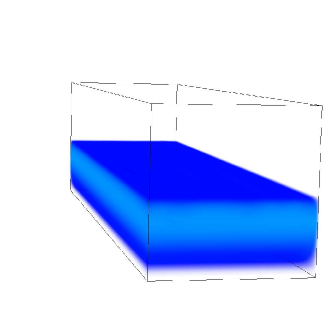
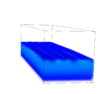
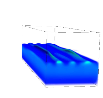
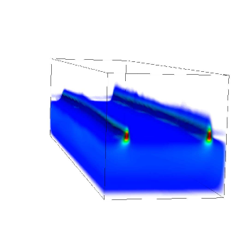
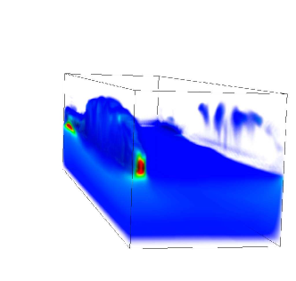
Figure 2: Volume renderings of $|\mathbf{B}|$ for a simulation with $M_{\gamma}=1$ at approximate times $t=46,98,123,267$ and $325$, respectively. This illustrates the temporal evolution of the magnetic field in a simulation of the buoyancy instability of a preconceived magnetic slab with magnetic pumping in the upper layer.

Volume rendering images illustrating the temporal evolution of our simulation with $M_{\gamma}=1$ for $|\mathbf{B}|$ are presented in Fig. 2. So far what we have discussed is identical to the evolution described in Matthews, Hughes & Proctor (1995) and Wissink et al. (2000), which is what we would expect until the field has risen far enough to reach the $\gamma$-interface. Once the buoyant magnetic structures reach $z\approx z_{i}$, the resulting evolution depends on the relative strength of the field compared to that which can be held down by the $\gamma$-pumping, i.e. whether $|\mathbf{B}_{h}|>B_{eq}$, which clearly depends on the value of $M_{\gamma}$ for the initial state. If $M_{\gamma}\ll 1$ downward pumping is unable to counteract the upward transport of magnetic flux due to buoyancy. In this regime, the rising magnetic structures are able to rise into the upper layer effectively unhindered, and on horizontal scales comparable to the initial instability.

The more interesting regime is when $M_{\gamma}\gtrsim 1$, since downward pumping is then efficient at holding down the bulk of the magnetic field, as must be the case in the Sun. However, localised pockets of magnetic field with strengths satisfying $|\mathbf{B}_{h}|>B_{eq}$ can still be produced. Several mechanisms are responsible for this. One is a nonlinear effect, in which rising pockets of magnetic field generate vortices, therefore the region in the vicinity of $z_{i}$ is subject to complicated interactions between them. In some cases, these interactions are able to concentrate magnetic flux below the interface, primarily horizontally, to produce localised pockets of strong field (we later illustrate this in a simulation with shear in Fig. 11). Two other effects which can locally concentrate the field are the vertical variation of the $\gamma$-pumping, which can amplify field through its nonzero divergence, together with the effect of buoyancy instabilities below the interface driving flux upwards into the interface. A combination of these effects can produce localised peak fields that satisfy $|\mathbf{B}_{h}|>B_{eq}$, and so are able to rise, even if the layer as a whole is contained because $M_{\gamma}\gtrsim 1$.

Rising pockets of magnetic field are ultimately sheared apart by interacting with the gas in the upper layer and do not rise far as coherent structures. Since they are predominantly toroidal structures, they are not transversally supported by magnetic tension, and are therefore easily destroyed (see e.g. Hughes et al. 1998; Hughes & Falle 1998). Magnetic structures that are arched in the lower layer become straightened as they rise up through the $\gamma$-transition region. This is because, although $\gamma$ is horizontally uniform, there exists a vertical transition region in which $\gamma$ increases with height. The peaks of the arches are therefore pushed downwards more strongly than the troughs, which straightens the field lines as they rise through this region. It must be noted that this is an artifact of our adopted profile of magnetic pumping, and arched magnetic structures could easily be produced if there were some horizontal variation in the strength of $\gamma$. In reality, arched magnetic structures could be produced either by the initial instability or its early nonlinear evolution, or by the action of turbulent motions in the convection zone on initially straight structures, with the latter being observed by Jouve & Brun (2009), for example.

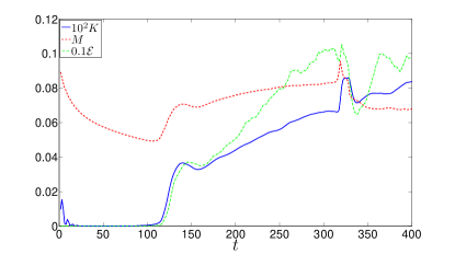
Figure 3: Temporal evolution of the volume-integrated magnetic energy $M$, kinetic energy $K$ and enstrophy $\mathcal{E}$, in a simulation with $M_{\gamma}=1$, where these quantities have been scaled as listed in the legend.

During this simulation, the potential energy of the initial configuration is transformed to kinetic energy of the initial instability. Almost immediately, the shearing motions of the field generate vortices through Kelvin-Helmholtz instabilities. Illustrated in Fig. 3, the integrated magnetic energy ($M=\int_{0}^{1}\langle\frac{1}{2}|\mathbf{B}|^{2}\rangle dz$, where we denote a horizontal average by $\langle X\rangle=\int\int Xdxdy$) initially builds until the instability has developed and localised strong field pockets start to rise into the upper layer (at $t\approx 110$). Once this occurs, the subsequent generation of vorticity is illustrated by the increase in kinetic energy ($K=\int_{0}^{1}\langle\frac{1}{2}\rho|\mathbf{u}|^{2}\rangle dz$) and enstrophy ($\mathcal{E}=\int_{0}^{1}\langle\frac{1}{2}|\nabla\times\mathbf{u}|^{2}\rangle dz$) within the computational domain for $t\gtrsim 110$. Afterwards, the initial instability dies out and viscous and ohmic diffusion result in a slow decay of the integrated energies. Since the influence of the (artificial) upper boundary becomes more important as the simulation progresses, we only analyse the results until $t\approx 400$.

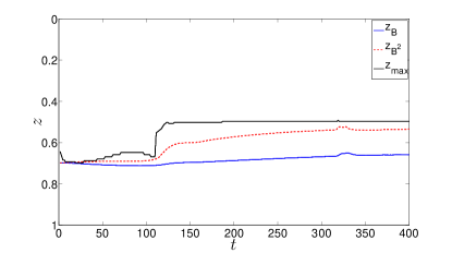
Figure 4: Temporal evolution of the peak magnetic field $z_{\mathrm{max}}$, the centre of magnetic field $z_{B}$, and the centre of magnetic energy $z_{B^{2}}$, in a simulation with $M_{\gamma}=1$.

It is instructive to define several measures to describe the spatial distribution of magnetic flux in the computational domain, and therefore understand the relative efficiencies of magnetic buoyancy and magnetic pumping. We can define the vertical location of the peak magnetic field, the centre of magnetic field (e.g. Wissink et al. 2000; Tobias et al. 2001), and the centre of magnetic energy, respectively, as

$$z_{\mathrm{max}} = \underbrace{\mathrm{max}}_{\mathbf{|B|}}\left\{z\right\},$$ (20)

$$z_{B} = \frac{\int_{0}^{1}z\langle B_{y}\rangle dz}{\int_{0}^{1}\langle B_{y}\rangle dz},$$ (21)

$$z_{B^{2}} = \frac{\int_{0}^{1}z\langle|\mathbf{B}|^{2}\rangle dz}{\int_{0}^{1}\langle|\mathbf{B}|^{2}\rangle dz}.$$ (22)

We plot these measures as a function of time in Fig. 4, where it can be seen that the peak field is located at a depth $z\approx z_{i}$. Note that the bulk of the field is held down in the lower layer, since $z_{B}>z_{i}$. This is a result of both the interaction between neighbouring vortices, which can act in concert to hold down the bulk of the field, as has been previously observed by Cattaneo & Hughes (1988), together with $\gamma$-pumping in the upper layer. Note that $z_{B^{2}}$ is located slightly higher than $z_{B}$. This difference can occur when either $\mathbf{B}$ contains appreciable $B_{x}$ or $B_{z}$ higher up, or alternatively if the field contains unsigned magnetic field in this region. The latter can be produced by the induction of small-scale field by vortices, which is most important at the top of the transition region. The depth of the peak field moves around chaotically because magnetic field is advected by vortical fluid motions near the interface, though it always remains near $z_{i}$.

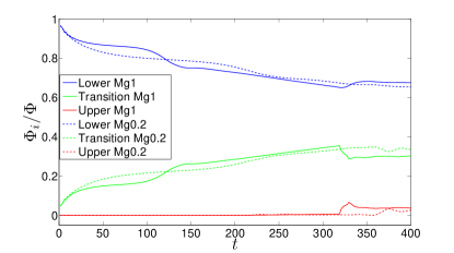
Figure 5: Temporal evolution of the magnetic flux fraction contained within the lower layer $\Phi_{L}/\Phi$, the transition region $\Phi_{T}/\Phi$ and the upper layer $\Phi_{U}/\Phi$, in a simulation with $M_{\gamma}=1$ (solid lines) and $M_{\gamma}=0.2$ (dashed lines).

We define the total magnetic flux, as well as the magnetic flux contained within the lower, transition and upper regions as

$$\Phi = \int_{0}^{1}\langle B_{y}\rangle dz,$$ (23)

$$\Phi_{U} = \int_{0}^{0.4}\langle B_{y}\rangle dz,$$ (24)

$$\Phi_{T} = \int_{0.4}^{0.6}\langle B_{y}\rangle dz$$ (25)

$$\Phi_{L} = \int_{0.6}^{1}\langle B_{y}\rangle dz.$$ (26)

We plot each of the last three normalised to the total $\Phi$ (which is a time varying quantity, primarily due to ohmic dissipation) at each time in Fig. 5. Magnetic pumping gradually pumps any flux out of the upper layer, competing against localised breakouts (and ohmic diffusion). The fraction of the magnetic flux contained in the upper layer is always less than approximately $5\%$ of the total initial flux, which reinforces the localised nature of the breakouts. In addition, the field is primarily of a diffuse nature in the upper layer because the coherence of the rising pockets of flux are not maintained. Note that $\Phi_{U}/\Phi$ is slightly smaller in the simulation with $M_{\gamma}=0.2$ than that with $M_{\gamma}=1$, which might seem surprising. This is because the amplification of field through the divergence of $\gamma$ near $z_{i}$ is weaker, whereas the bulk of the field is held down as efficiently by vortices.

To summarise the results of this section, we find that although the nonlinear evolution of buoyancy instabilities of a preconceived magnetic slab can produce localised pockets of strong field which are able to rise up against $\gamma$-pumping, the bulk of the field is held down in the lower layer. This is a result of a combination of the interactions between vortices and $\gamma$-pumping in the upper layer. A combination of these effects might be responsible for holding down the bulk of the solar toroidal field, allowing only localised breakouts into the convection zone.

4 Numerical Model with shear

The simulations described so far have assumed a preconceived horizontal magnetic field configuration in the initial state. From here on, we extend our study of magnetic pumping to examine the effect of its addition on the generation of the horizontal magnetic layer by the action of vertical shear on an initially uniform vertical field, following VB08 and SBP09. This shear is designed to mimic the radial shear in the tachocline. We do not consider any latitudinal (horizontal) shear because this is inferred to be much weaker than the radial component (e.g. Christensen-Dalsgaard & Thompson 2007). Our adopted vertical shear profile is

$$\mathbf{U}_{0}=\frac{U_{m}}{2}\left[1+\tanh\left[(\Delta z_{s})^{-1}\left(z_{s}-z\right)\right]\right]\mathbf{e}_{y}.$$ (27)

We choose $U_{m}\ll 1$ so that this shear is subsonic, as is appropriate for the tachocline. Unfortunately, it is numerically feasible to simulate the tachocline shear only when it is hydrodynamically unstable to a Kelvin-Helmholtz type instability, in which case the instabilities are standard, i.e. not double-diffusive, instabilities. This is because capturing the double-diffusive instabilities would require very high resolution. This means that it is only possible to perform a parameter survey when $Ri=\mathrm{min}\left\{N^{2}/\left(\frac{d\mathbf{U_{0}}}{dz}\right)^{2}\right\}\lesssim\frac{1}{4}$, which is unlikely to be valid in the Sun (Gough, 2007). Nevertheless, the resulting Kelvin-Helmholtz instabilities are suppressed when the induced horizontal field strength becomes sufficiently large (e.g. SBP09). This is usually well before the onset of any magnetic buoyancy instabilities, so it should not significantly influence the dynamics that we are interested in (except by producing inhomogeneities in the magnetic layer along the direction of the induced field).

In previous work, VB08 and VB09 have studied a similar problem and found some difficulties in maintaining the initial shear profile. They used an applied stress, which is designed to counter viscous decay, to maintain the shear. However, this is not able to maintain the background shear in the presence of strong magnetic fields, and the shear profile that remains at the end of their simulations did not match that of the desired (initial) profile (see VB08 Fig. 13). This motivated us to consider a different approach which will maintain the desired shear profile and might therefore be better at capturing the important effects of tachocline shear on our problem (particularly for long duration simulations). Our approach is to decompose the velocity field into $\mathbf{u}=\mathbf{u}^{\prime}+\mathbf{U}_{0}$, and consider $\mathbf{U}_{0}$ to be steady, i.e. we consider the tachocline to be externally maintained. We neglect the back-reaction of $\mathbf{u}^{\prime}$ on $\mathbf{U}_{0}$, and solve Eqs. 1–5 for $\mathbf{u}^{\prime}$ instead of the total velocity field $\mathbf{u}$. This has the advantage that the underlying shear profile is not affected by the magnetic buoyancy instabilities that we are interested in studying.

We now outline the modifications to the numerical model outlined in §2 which allow this problem to be simulated. The initial state is now a (single) polytropic layer permeated by a uniform vertical magnetic field $\mathbf{B}=B_{0}\mathbf{e}_{z}$. In the absence of shear ($\mathbf{U}_{0}=\mathbf{0}$), this is an equilibrium solution (neglecting diffusion). However, when our adopted shear profile is present, the initial state is no longer an equilibrium configuration because the vertical field is stretched by the shear to produce a horizontal field. The instability of this field will produce magnetic structures that buoyantly rise into the upper layer, where they are acted upon by downward pumping, which is implemented as in §2.1.

We explicitly add additional terms into Eqs. 1–4 that take into account the forcing of the flow by the background shear $\mathbf{U}_{0}$. These terms are

$$F_{\rho} = -\mathbf{U}_{0}\cdot\nabla\rho,$$ (28)

$$\mathbf{F}_{\mathbf{u}} = -\mathbf{U}_{0}\cdot\nabla\mathbf{u}^{\prime}-\mathbf{u}^{\prime}\cdot\nabla\mathbf{U}_{0},$$ (29)

$$F_{T} = -\mathbf{U}_{0}\cdot\nabla T,$$ (30)

$$\mathbf{F}_{\mathbf{B}} = \nabla\times\left(\mathbf{U}_{0}\times\mathbf{B}\right),$$ (31)

which must be added onto the right hand sides of Eqs. 1–4 (in that order), where we have taken into account that $\nabla\cdot\mathbf{U}_{0}=0$.

4.1 Parameters adopted

The parameters adopted for our calculations with shear are outlined in Table 2, where it can be noted that most of the parameters remain unchanged from the model in §2 that we have summarised in Table 1.

Parameter	Description	Value
$m$	Polytropic index	1.6
$\theta$	Thermal stratification	2.0
$C_{K}$	Thermal diffusivity	0.01
$\zeta_{0}$	Magnetic diffusivity	0.01
$\sigma$	Prandtl number	0.005
$F$	Magnitude of magnetic energy	$10^{-5}$
$\gamma_{m}$	Magnetic pumping strength	Various
$z_{i}$	Bottom of pumping layer	0.5
$(\Delta z_{i})^{-1}$	Width of transition region	30.0
$U_{m}$	Magnitude of shear	0.1
$z_{s}$	Location of shear	0.75
$(\Delta z_{s})^{-1}$	Width of shear region	30.0
$\lambda_{x},\lambda_{y}$	Box horizontal aspect ratio	$1,4$

Table 2: Parameter values for the simulations with shear.

In the presence of shear, once magnetic field gradients become sufficient for magnetic buoyancy instabilities to occur, the resulting evolution will depend on the Alfvénic Mach number of the shear-generated magnetic layer. The strength of the magnetic field in the layer will grow according to

$$B_{y}\approx\frac{B_{z}U_{m}}{2\Delta z_{s}}t,$$ (32)

until such a time as the layer has spread due to the slow propagation of Alfvén waves along the initial vertical field. The associated timescale for this process is $t\approx\Delta z_{s}/(2v_{A})$, which is the vertical Alfvén travel time across half of the shear region. In our units, the peak field is therefore $\mathrm{max}(B_{y})\approx U_{m}\sqrt{\frac{\rho(z_{s})}{F}}$. This means that our parameter $M_{\gamma}$ from § 2 is equivalent to

$$M_{\gamma}=\frac{B_{eq}}{\mathrm{max}(B_{y})}=\frac{\gamma_{m}}{\mathrm{max}(B_{y})}\sqrt{\frac{\rho(z_{i})}{F}}\approx\frac{\gamma_{m}}{U_{m}}\sqrt{\frac{\rho(z_{i})}{\rho(z_{s})}}.$$ (33)

The evolution of buoyantly unstable field which reaches the upper layer will therefore depend on the parameter

$$M_{U}=\frac{\gamma_{m}}{U_{m}},$$ (34)

which will play an analogous role to $M_{\gamma}$ from § 2 (the density ratio is approximately unity). Noting that $(1/2)\rho\gamma_{m}^{2}$ is likely to be comparable to (though smaller than) the kinetic energy of the convection (and remembering that $\gamma$ is not an actual fluid velocity in our mean-field interpretation), $M_{U}^{2}$ is a measure of the ratio of the kinetic energy of the convection to that of the shear. If $M_{U}\lesssim 1$, we would expect shear to generate sufficiently strong horizontal magnetic fields for the resulting rising structures produced by magnetic buoyancy to be able to overcome the downward pumping. Alternatively, if $M_{U}\gtrsim 1$, we would expect the generated field to produce buoyant structures that are too weak to overcome the downward pumping, unless magnetic flux can be locally concentrated so that $|\mathbf{B}_{h}|>B_{eq}$. As in the simulations without shear, we study various values of $M_{U}$ either side of unity by fixing $U_{m}$ and varying $\gamma_{m}$.

Since the shear is designed to represent the radial shear in the tachocline, we choose the width of the shear region to be much thinner than a pressure scale height, with $\Delta z_{s}\approx 0.03\ll 1$. The magnitude of the shear is subsonic, with $U_{m}=0.1$, though this is still larger than in the Sun so that the evolution can be fully captured within a sensible run time. Note that this shear is hydrodynamically unstable, with $Ri\approx 0.074<0.25$. This means that the shear excites vortices (aligned in the $x$-direction) through Kelvin-Helmholtz type instabilities. Since these instabilities are unwanted, we try to partially reduce their effect by having a small fluid Reynolds number for the shear of $Re\sim 66$. In any case, the resulting vortices are eventually suppressed by the induced horizontal field.

5 Results: shear production of a magnetic layer, its instability and interaction with downward pumping

In this section we describe the results of a set of simulations with shear using the numerical model outlined in §4. First we describe the temporal evolution for our fiducial case, which has $M_{U}=1$. We then discuss the effects of varying $M_{U}$.

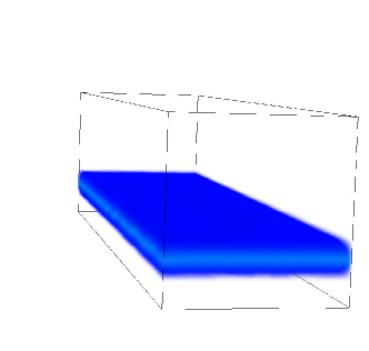
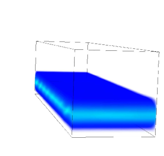
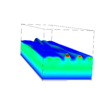
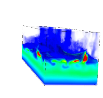
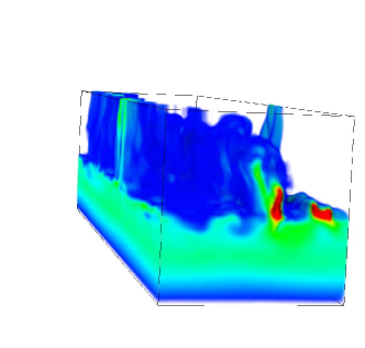
Figure 6: Volume renderings of $|\mathbf{B}|$ for a simulation with $M_{U}=1$ at approximate times $t=15,42,160,177$ and $200$, respectively. This illustrates the temporal evolution of the magnetic field in a simulation of the buoyancy instability of a shear-generated magnetic slab with magnetic pumping in the upper layer, using $M_{U}=1$.

As the simulation begins, vertical shear acting on the uniform vertical magnetic field generates a magnetic layer aligned in the (negative) $y$-direction (for positive $U_{m}$). In the initial stages this field grows in magnitude and also gradually expands due to the vertical propagation of Alfvén waves along the initial field. A hydrodynamic Kelvin-Helmholtz type instability sets in from our prescribed shear flow, which generates vortices aligned in the $x$-direction. This occurs because our adopted shear is hydrodynamically unstable, as we explained in §4. However, as the magnetic field in the layer grows, Lorentz forces act back on the resulting flow and hinder further development of the instability (e.g. SBP09). It therefore eventually dies out as the field strength exceeds a critical value, leaving behind only some weak inhomogeneities in the $y$-direction. Volume rendering images illustrating the temporal evolution of our simulation with $M_{U}=1$ for $|\mathbf{B}|$ are presented in Fig. 6.

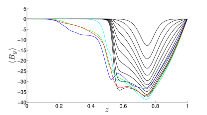
Figure 7: Horizontally integrated $B_{y}$ in a simulation with $M_{U}=1$ for multiple time intervals between $t\approx 15-150$ until the field has built up a sufficient gradient near $z_{i}$ for buoyancy instabilities to set in at this location (black lines), together with the same quantity after onset of buoyancy instability there, at approximate times $t=163$ (light blue), $192$ (green), $222$ (red) and $266$ (dark blue). The maximum field amplitude in the shear region is approximately equal to $U_{m}/\sqrt{F}$.

Once magnetic field gradients become sufficiently strong, buoyancy instabilities occur in the upper parts of this expanding magnetic layer. These are of two-dimensional interchange type (like in § 3), which are expected to be least affected by the addition of an aligned shear flow (Tobias & Hughes, 2004). At the same time, vertically propagating Alfvén waves, together with a small amount of ohmic diffusion, spread the horizontal magnetic field throughout the lower layer. Since the field is confined from above at the $\gamma$-interface, it remains well confined within the lower layer unless its magnitude can locally exceed $B_{eq}$. For this to occur once the buoyant magnetic structures, or the bulk of the expanding magnetic layer, first reach the interface requires $M_{U}\ll 1$, otherwise the bulk of the field is held down below the $\gamma$-interface. The maximum field strength in the shear-generated layer reaches $B_{y}\sim\frac{U_{m}}{\sqrt{F}}\sim 35$. This can be seen in Fig. 7, which displays the horizontally-integrated vertical profile of $B_{y}$ as the field builds underneath the interface for $t=15-150$ (thin black lines). The field for $z\gtrsim z_{i}$ builds up to approximately this value due to the combined action of shear at generating the magnetic layer and $\gamma$-pumping at holding down the field.

There are several important effects resulting from the addition of $\gamma$-pumping in the upper layer. The simplest of these is to hold down the bulk of the field in the lower layer. If $\gamma$-pumping is not present, the bulk of the field, together with any buoyantly unstable pockets of field, continue to expand throughout the upper layer. Since the Sun has some means of holding back field until it reaches a certain strength, we require some mechanism to hold down weak field. In our simulations magnetic flux pumping in the upper layer (“the convection zone”) provides such a mechanism, with only localised pockets of strong field able to rise above $z\approx z_{i}$. Unlike in §3, where the interactions between vortices are also capable of holding down the bulk of the magnetic field, in these simulations the magnetic layer would continue to expand because of the slow vertical propagation of Alfvén waves along the initial field. We therefore require $\gamma$-pumping to hold down the bulk of the field in these simulations.

Another important effect of $\gamma$-pumping is to produce strong vertical magnetic field gradients in the vicinity of $z_{i}$ (see Fig. 7), which induces buoyancy instabilities at this location. These result from the vertical gradients of $\gamma$, and provide an additional way to produce strong field gradients, and therefore induce (in our case non-diffusive) buoyancy instabilities, without requiring strong (i.e. hydrodynamically unstable) shear (e.g. VB08). Once the upper interface of the magnetic layer is perturbed by the instability, the important factor is the relative strength of the field in the rising magnetic structures to that which can be held down by the $\gamma$-pumping, i.e. whether $|\mathbf{B}_{h}|>B_{eq}$.

As in §3, rising pockets of magnetic field generate vortices, so the vicinity of $z_{i}$ is subject to complicated interactions between them. In some cases, the resulting fluid motions are able to concentrate the field horizontally below the interface into localised pockets of strong field (an example of this is plotted later in Fig. 11). Note that the spatial scales of these magnetic structures are not necessarily the same as those of the initial buoyancy instability. A combination of the above effects, together with the continual forcing of the horizontal layer by the shear, can produce localised peak fields that satisfy $|\mathbf{B}_{h}|>B_{eq}$. Such strong pockets can rise into the upper layer. As before, rising flux structures are eventually sheared apart by shear interactions with the gas in the upper layer, and do not rise far as coherent structures.

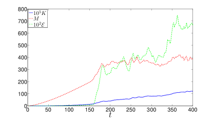
Figure 8: Temporal evolution of the volume-integrated magnetic energy $M$, kinetic energy $K$ and enstrophy $\mathcal{E}$, in a simulation with shear and $M_{U}=1$, where these quantities have been scaled as listed in the legend.

As is illustrated in Fig. 8, the magnetic energy builds until it reaches its peak value just before the field below the interface has been sufficiently concentrated to be able to break out into the upper layer. Once buoyancy instabilities occur, the resulting local shear excites vortices, thereby increasing $K$ and $\mathcal{E}$. Since we are constantly forcing the system through the steady shear flow $\mathbf{U}_{0}$, the magnetic energy oscillates about an approximately constant value, and does not appreciably decay throughout the simulation. We analyse the results until $t\approx 400$, after which the influence of the upper boundary becomes important.

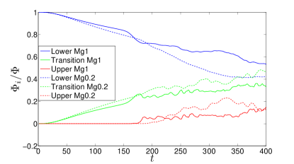
Figure 9: Temporal evolution of the magnetic flux fraction contained within the lower layer $\Phi_{L}/\Phi$, the transition region $\Phi_{T}/\Phi$ and the upper layer $\Phi_{U}/\Phi$, in a simulation with $M_{\gamma}=1$ (solid lines) and $M_{\gamma}=0.2$ (dashed lines).

We plot the flux fractions contained in each layer normalised to the total $\Phi$ (which is a time varying quantity due to shear production and ohmic dissipation) at each time in Fig. 9. This figure shows that the magnetic flux is initially produced and contained within the lower layer until the field has expanded and reached $z\approx z_{i}$. Afterwards, magnetic flux is primarily stored in the lower layer and transition region, with only a few localised outbursts transporting flux into the upper layer. We stress the localised nature of these pockets of field that rise into the upper layer, since the bulk of the field is well confined within the lower layer (i.e. $|\Phi_{U}|\ll|\Phi|$ at all times). We also plot the various measures of the distribution of magnetic field defined by Eqs. 20–22 as a function of time in Fig. 10, where it can be seen that they are each located within the transition region. This is the case even when strong localised breakouts are protruding flux into the upper layer. Note that again $z_{B^{2}}$ is located slightly higher than $z_{B}$. The peak magnetic field always remains at $z\approx z_{i}$.

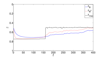
Figure 10: Temporal evolution of the peak magnetic field $z_{\mathrm{max}}$, the centre of magnetic field $z_{B}$, and the centre of magnetic energy $z_{B^{2}}$ for a simulation with $M_{U}=1$.

5.1 Variation of $M_{U}$

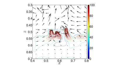
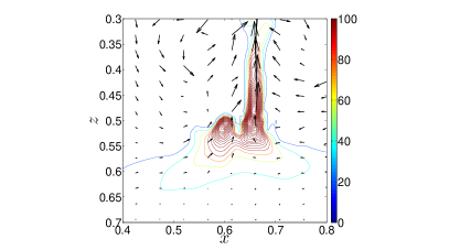
Figure 11: Contour plot of $|\mathbf{B}|$, together with velocity vectors at equally spaced points in a region of the $xz$-plane, in a simulation with $M_{U}=2$ at approximate times $t=166$ (left) and $169$ (right). This illustrates the concentration of magnetic flux in the transition region by vortical fluid motions, which can produce localised pockets of strong magnetic field with strengths sufficient to rise into the upper layer.

We have varied $M_{U}$ and looked at various values either side of unity to study the evolution in cases where the kinetic energy of the shear does and does not exceed that associated with the downward pumping. In the $M_{U}>1$ regime, we might expect the shear-generated field to be unable to reach strengths sufficient for buoyant rise into the upper layer. However, this neglects the concentration of horizontal magnetic flux by vortical fluid motions, produced in the nonlinear stages of evolution of the system. We have observed the field to be locally concentrated and to rise into the upper layer in localised breakouts even when $M_{U}=4$, i.e. the kinetic energy of the shear is significantly less than $(1/2)\rho\gamma_{m}^{2}$, and therefore also smaller than the kinetic energy of the convection, by more than an order of magnitude. In Fig. 11, we show an example of the concentration of field in the transition region by vortical fluid motions in the vicinity of $z_{i}$ in a simulation with $M_{U}=2$. A localised pocket of field with a strength $\mathbf{B}_{h}\gtrsim 100\sim B_{eq}$ is produced, which then breaks out into the upper layer.

Note that in these simulations $\gamma_{m}$ is not as strongly subsonic as it is likely to be in the tachocline. The plasma $\beta$ required for a pocket of magnetic field to rise is therefore much smaller than we expect in reality, and for the strongest field $\beta\ll 1$. The magnetic pressure is therefore able to evacuate the gas within a grid cell, and this becomes particularly important in the strongest field pockets produced when $M_{U}>1$. This causes the timestep to decrease towards zero to satisfy the Courant-Friedrichs-Lewy stability constraint, and the numerical code to fail. This limits the maximum value of $M_{U}$ that we can simulate to $M_{U}\lesssim 5$, unless we either increase the resolution or reduce the initial values of $\gamma_{m}$ and $U_{m}$, which both require greater computational resources. Nevertheless, simulations with $1\lesssim M_{U}\lesssim 5$ indicate that it is possible in this regime for a combination of $\gamma$-pumping at holding down (and amplifying) the field, and vortical fluid motions at concentrating magnetic flux, to produce pockets with sufficient field strength to be able to rise into the upper layer.

6 Conclusions

In this paper we have studied the interaction between magnetic buoyancy instabilities and magnetic flux pumping in simplified numerical models of the solar tachocline. We have adopted an idealised “mean-field” model of magnetic flux pumping, in which a spatially uniform and temporally constant downward advective velocity $\gamma$ for the magnetic field is added into the induction equation in an upper layer, with no flux pumping present in the lower layer. This situation is designed to crudely represent the effects of magnetic flux pumping in the lower parts of the convection zone, which overly a stable radiative region containing a layer of buoyantly unstable toroidal magnetic field.

We first studied the addition of a simple $\gamma$-effect into simulations of the instability of a preconceived horizontal slab of magnetic field, extending the calculations of Cattaneo & Hughes (1988) and Matthews, Hughes & Proctor (1995). In this problem, the initial configuration is a magnetostatic equilibrium, perturbed by small thermal perturbations, which induce Rayleigh-Taylor type instabilities at the top of the magnetic layer. The resulting magnetic mushrooms rise until they reach the pumping layer. The effect of this layer on the resulting evolution depends on the ratio of the downward pumping velocity to the Alfvén speed of the magnetic field, that we denote $M_{\gamma}$. When $M_{\gamma}\gtrsim 1$, the magnetic flux pumping effectively holds down the bulk of the field, only allowing localised pockets of strong field to rise, which have been concentrated by vortical fluid motions.

Since the Rayleigh-Taylor type instabilities of a toroidal magnetic layer do not have a weak field cut off, and occur for any field strength (in the absence of diffusion), there must exist a mechanism to hold down the field until it can exceed a critical strength (Hughes, 2007). Magnetic flux pumping can provide one solution to this problem, since its addition immediately prevents fields weaker than equipartition strength from rising into the convection zone. If $M_{\gamma}\gtrsim 1$ in reality, then magnetic flux pumping can explain why the bulk of the field is stored in the radiative interior, with only localised pockets of strong field able to rise through the convection zone towards the surface. It is interesting to note that our simulations in this regime show that the instability of a uniform initial field lying underneath a layer with uniform downward magnetic flux pumping can produce localised clumps of field that rise some distance into the upper layer.

We also studied the addition of a $\gamma$-effect into simulations of the instability of a shear-generated magnetic layer, continuing calculations in the spirit of VB08 and SBP09. In this problem, we consider radial tachocline shear to induce a toroidal magnetic layer, which then becomes buoyantly unstable. The effect of magnetic flux pumping on this problem has several important contributions. One is to produce strong magnetic field gradients near the interface of the pumping layer. This strongly enhances the likelihood of buoyancy instabilities occurring in this region, and is therefore one method of inducing such instabilities when the toroidal magnetic layer is forced by a weak, hydrodynamically stable, tachocline shear. We do not, therefore, require strong shear for magnetic buoyancy instabilities to be excited (c.f. VB08; VB09).

The evolution in cases with shear depends on the ratio of the pumping velocity to the shear velocity, that we denote $M_{U}$. One interesting result of these simulations is that even in the case in which $M_{U}>1$ the shear was able to produce localised rising pockets of field. This is interesting because the tachocline shear is probably maintained at a level such that it has a similar mean kinetic energy density as the convection. Therefore, the toroidal field that is produced by this shear might be expected to have at most equipartition strength with the convective downflows. Since we have observed localised pockets of magnetic flux to rise in the regime with $M_{U}>1$, because field is amplified by the combined action of concentration by vortical fluid motions, shear at forcing the layer and $\gamma$-pumping at holding it down (and amplifying it through its non-zero divergence), this indicates that the shear is not necessarily required to be more energetic than the convection for superequipartition fields to be produced by magnetic buoyancy instabilities. Somewhat paradoxically, magnetic flux pumping (or rather its strong radial gradients near the tachocline) may in fact be an essential ingredient in producing localised pockets of superequipartition field that are able to rise up through the convection zone and to the solar surface.

One important problem, which we have not attempted to address here, is how does the instability produce fields that are sufficiently helical for the resulting magnetic structures to survive their passage through the convection zone? The solution to this problem will require consideration of initial fields that are spatially inhomogeneous and not unidirectional. In addition, we have modelled the effects of magnetic flux pumping in the crudest possible way. Indeed, this calculation does not in any sense aim to be the last word on the matter. Rather, it should be seen as a pilot project which has the limited aim of establishing the efficacy of a mechanism for flux concentration. Now that this mechanism has been shown to have validity the next step is a fully resolved calculation for more general initial fields and a turbulent convection zone in which the effect can be put on a proper quantitative footing. This work is presently in progress.

References

- Acheson (1979) Acheson D. J., 1979, Solar Physics, 62, 23
- Arter (1983) Arter W., 1983, Journal of Fluid Mechanics, 132, 25
- Arter et al. (1982) Arter W., Proctor M. R. E., Galloway D. J., 1982, MNRAS, 201, 57P
- Brummell et al. (2002) Brummell N., Cline K., Cattaneo F., 2002, MNRAS, 329, L73
- Bushby & Houghton (2005) Bushby P. J., Houghton S. M., 2005, MNRAS, 362, 313
- Cattaneo & Hughes (1988) Cattaneo F., Hughes D. W., 1988, Journal of Fluid Mechanics, 196, 323
- Cattaneo et al. (1988) Cattaneo F., Hughes D. W., Proctor M. R. E., 1988, Geophysical and Astrophysical Fluid Dynamics, 41, 335
- Christensen-Dalsgaard & Thompson (2007) Christensen-Dalsgaard J., Thompson M. J., 2007, in D. W. Hughes, R. Rosner, & N. O. Weiss ed., The Solar Tachocline Observational results and issues concerning the tachocline. p. 53
- Cline et al. (2003) Cline K. S., Brummell N. H., Cattaneo F., 2003, ApJ, 599, 1449
- Crow (1970) Crow S. C., 1970, AIAA Journal, 8, 2172
- Dorch & Nordlund (2001) Dorch S. B. F., Nordlund Å., 2001, A& A, 365, 562
- Drobyshevski & Yuferev (1974) Drobyshevski E. M., Yuferev V. S., 1974, Journal of Fluid Mechanics, 65, 33
- Galloway & Proctor (1983) Galloway D. J., Proctor M. R. E., 1983, Geophysical and Astrophysical Fluid Dynamics, 24, 109
- Gilman (1970) Gilman P. A., 1970, ApJ, 162, 1019
- Gough (2007) Gough D., 2007, in D. W. Hughes, R. Rosner, & N. O. Weiss ed., The Solar Tachocline An introduction to the solar tachocline. p. 3
- Guerrero & Käpylä (2011) Guerrero G., Käpylä P., 2011, ArXiv e-prints
- Hughes (2007) Hughes D. W., 2007, in D. W. Hughes, R. Rosner, & N. O. Weiss ed., The Solar Tachocline Magnetic buoyancy instabilities in the tachocline. p. 275
- Hughes & Falle (1998) Hughes D. W., Falle S. A. E. G., 1998, ApJL, 509, L57
- Hughes et al. (1998) Hughes D. W., Falle S. A. E. G., Joarder P., 1998, MNRAS, 298, 433
- Hughes & Proctor (1988) Hughes D. W., Proctor M. R. E., 1988, Annual Review of Fluid Mechanics, 20, 187
- Jones et al. (2010) Jones C. A., Thompson M. J., Tobias S. M., 2010, Space Science Reviews, 152, 591
- Jouve & Brun (2009) Jouve L., Brun A. S., 2009, ApJ, 701, 1300
- Kitchatinov & Rüdiger (2008) Kitchatinov L. L., Rüdiger G., 2008, Astronomische Nachrichten, 329, 372
- MacGregor & Charbonneau (1999) MacGregor K. B., Charbonneau P., 1999, ApJ, 519, 911
- Matthews et al. (1995) Matthews P. C., Hughes D. W., Proctor M. R. E., 1995, ApJ, 448, 938
- Matthews et al. (1995) Matthews P. C., Proctor M. R. E., Weiss N. O., 1995, Journal of Fluid Mechanics, 305, 281
- Miesch et al. (2008) Miesch M. S., Brun A. S., De Rosa M. L., Toomre J., 2008, ApJ, 673, 557
- Moffatt (1978) Moffatt H. K., 1978, Magnetic field generation in electrically conducting fluids
- Moffatt (1983) Moffatt H. K., 1983, Reports on Progress in Physics, 46, 621
- Ossendrijver (2003) Ossendrijver M., 2003, A&A Review, 11, 287
- Ossendrijver et al. (2002) Ossendrijver M., Stix M., Brandenburg A., Rüdiger G., 2002, A& A, 394, 735
- Parker (1975) Parker E. N., 1975, ApJ, 198, 205
- Rädler (1968) Rädler K. H., 1968, Zeitschrift Naturforschung Teil A, 23, 1851
- Rogers (2011) Rogers T. M., 2011, ApJ, 733, 12
- Schmitt & Rosner (1983) Schmitt J. H. M. M., Rosner R., 1983, ApJ, 265, 901
- Silvers et al. (2009) Silvers L. J., Bushby P. J., Proctor M. R. E., 2009, MNRAS, 400, 337
- Silvers et al. (2009) Silvers L. J., Vasil G. M., Brummell N. H., Proctor M. R. E., 2009, ApJL, 702, L14
- Silvers et al. (2010) Silvers L. J., Vasil G. M., Brummell N. H., Proctor M. R. E., 2010, Proceedings of the International Astronomical Union, 6, 218
- Spiegel & Weiss (1980) Spiegel E. A., Weiss N. O., 1980, Nature, 287, 616
- Tao et al. (1998) Tao L., Proctor M. R. E., Weiss N. O., 1998, MNRAS, 300, 907
- Tobias & Weiss (2007) Tobias S., Weiss N., 2007, in D. W. Hughes, R. Rosner, & N. O. Weiss ed., The Solar Tachocline The solar dynamo and the tachocline. p. 319
- Tobias et al. (1998) Tobias S. M., Brummell N. H., Clune T. L., Toomre J., 1998, ApJL, 502, L177
- Tobias et al. (2001) Tobias S. M., Brummell N. H., Clune T. L., Toomre J., 2001, ApJ, 549, 1183
- Tobias & Hughes (2004) Tobias S. M., Hughes D. W., 2004, ApJ, 603, 785
- Vasil & Brummell (2008) Vasil G. M., Brummell N. H., 2008, ApJ, 686, 709
- Vasil & Brummell (2009) Vasil G. M., Brummell N. H., 2009, ApJ, 690, 783
- Vergassola & Avellaneda (1997) Vergassola M., Avellaneda M., 1997, Physica D Nonlinear Phenomena, 106, 148
- Weiss et al. (2004) Weiss N. O., Thomas J. H., Brummell N. H., Tobias S. M., 2004, ApJ, 600, 1073
- Wissink et al. (2000) Wissink J. G., Hughes D. W., Matthews P. C., Proctor M. R. E., 2000, MNRAS, 318, 501
- Zeldovich (1957) Zeldovich Y. B., 1957, Sov. Phys. JETP