Structural Variation of Molecular Gas in the Sagittarius Arm and Inter-Arm Regions

Abstract

We have carried out survey observations toward the Galactic plane at $l\approx 38\arcdeg$ in the ${}^{12}{\rm CO}$ and ${}^{13}{\rm CO}$ $J=1\mbox{--}0$ lines using the Nobeyama Radio Observatory 45-m telescope. A wide area ($0\fdg 8\times 0\fdg 8$) was mapped with high spatial resolution ($17\arcsec$). The line of sight samples the gas in both the Sagittarius arm and the inter-arm regions. The present observations reveal how the structure and physical conditions vary across a spiral arm. We classify the molecular gas in the line of sight into two distinct components based on its appearance: the bright and compact B component and the fainter and diffuse (i.e., more extended) D component. The B component is predominantly seen at the spiral arm velocities, while the D component dominates at the inter-arm velocities and is also found at the spiral arm velocities. We introduce the brightness distribution function and the brightness distribution index (BDI, which indicates the dominance of the B component) in order to quantify the map’s appearance. The radial velocities of BDI peaks coincide with those of high ${}^{12}{\rm CO}\;J=3\mbox{--}2/^{12}{\rm CO}\;J=1\mbox{--}0$ intensity ratio (i.e., warm gas) and H II regions, and tend to be offset from the line brightness peaks at lower velocities (i.e., presumably downstream side of the arm). Our observations reveal that the gas structure at small scales changes across a spiral arm: bright and spatially confined structures develop in a spiral arm, leading to star formation at downstream side, while extended emission dominates in the inter-arm region.

1 Introduction

The interstellar medium (ISM) plays an important role in galaxies: stars, the principal constituent of galaxies, are born from and return matter to the ISM. Since most neutral ISM is molecular in the inner part of galaxies (e.g., Dame, 1993; Sofue, Honma, & Arimoto, 1995; Honma, Sofue, & Arimoto, 1995; Koda et al., 2009) and stars form in dense molecular clouds, the studies of the distribution, spatial structures, and physical conditions of molecular gas are essential to understand the star-forming activities in galaxies. The Milky Way Galaxy is the unique target for resolving sub-pc structures of molecular gas with radio telescopes due to its proximity.

Some extensive mapping surveys of the Galactic disk in CO emission lines have been made since Scoville & Solomon (1975) and Gordon & Burton (1976). Two historic ${}^{12}{\rm CO}\;J=1\mbox{--}0$ surveys are the Columbia-CfA survey (Dame et al., 1987; Dame, Hartmann, & Thaddeus, 2001, and references therein) and the Massachusetts-Stony Brook Galactic Plane CO Survey (Sanders et al., 1986; Clemens et al., 1986). These surveys made use of the Columbia-CfA 1.2-m and the Five College Radio Astronomy Observatory (FCRAO) 14-m telescopes, providing an angular resolutions of $8\arcmin$ and $45\arcsec$, respectively. The first Galactic quadrant (and portions of adjacent quadrants) was mapped in the optically thinner isotopologue ${}^{13}{\rm CO}\;J=1\mbox{--}0$ line by the Bell Laboratories survey (Lee et al., 2001) with their 7-m telescope ($103\arcsec$ resolution) and the Boston University-FCRAO Galactic Ring Survey (Jackson et al., 2006) with the 14-m telescope. Surveys in higher-$J$ transitions (e.g., ${}^{12}{\rm CO}\;J=2\mbox{--}1$ by Sakamoto et al., 1995, 1997) were also made to diagnose the physical conditions of the gas.

These surveys have revealed the basic properties of molecular gas, such as its large-scale distribution in the Galaxy (Dame et al., 1986; Clemens, Sanders, & Scoville, 1988), and the presence of discrete molecular entities, i.e., giant molecular clouds (Solomon et al., 1979). There were many studies focused on identifying discrete molecular clouds and determining their physical/statistical properties (e.g., mass spectrum and the size-linewidth relation: Sanders et al., 1985; Solomon et al., 1987) and of substructures within them (e.g., Simon et al., 2001). Solomon, Sanders, & Rivolo (1985); Sanders et al. (1985); Scoville et al. (1987) studied the distribution of molecular clouds in the first Galactic quadrant. Although the catalogued clouds were distributed rather uniformly in the longitude-velocity ($l$-$v$) plane, they found that a subset of the clouds, “warm” or “hot” clouds with high brightness temperatures, followed clear $l$-$v$ patterns. The patterns agreed with those traced by H II regions and were considered as spiral arms. This might reflect the variation of the characteristics of the clouds affected by the galactic structures.

Previous surveys employed sparse spatial sampling and/or low resolution (on the order of arcminutes). Recently developed instruments have enabled us to perform Nyquist-sampled, high-resolution (tens of arcseconds) survey observations over wide fields (e.g., Jackson et al., 2006). With the high quality data, we would like to re-evaluate the picture of molecular content in the Galaxy. In particular, is there a way to study the spatial structures and the properties of the gas without decomposing it into clouds or their substructures, since the decomposition inevitably omits a part of the emission which may be important.

In this paper we present the results from our observations in the ${}^{12}{\rm CO}$ and ${}^{13}{\rm CO}$ $J=1\mbox{--}0$ lines with the Nobeyama Radio Observatory (NRO) 45-m telescope, proposing an alternative, complementary method to study the spatial structure of the gas at a sub-pc resolution. The method is based on the histogram of the brightness temperature of the line emission, or the brightness distribution function. We show how we selected the field, at $l\approx 38\arcdeg$, in Section 2. The observations and the data reduction process are described in Section 3. In Section 4 the velocity channel maps are presented. Then we characterize the observed line brightness, and discuss how the characteristics of the gas change across the spiral arms.

2 Field Selection

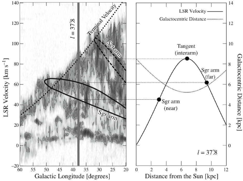
Figure 1: (a) Loci of the Sgr arm (solid line) and the Sct arm (dashed line) by Sanders et al. (1985) overlaid on the ${}^{12}{\rm CO}\;J=1\mbox{--}0$ longitude-velocity diagram (Dame, Hartmann, & Thaddeus, 2001). The tangent velocity for the $220\;{\rm km\;s^{-1}}$ flat rotation is also shown (dotted line). The observed line of sight is shaded. (b) LSR velocity (solid line; left ticks) and Galactocentric distance (dashed line; right ticks) as functions of distance from the Sun toward $l=37\fdg 8$.

Fig. 1a shows the longitude-velocity diagram of the ${}^{12}{\rm CO}\;J=1\mbox{--}0$ line (Dame, Hartmann, & Thaddeus, 2001). The loci of the Sagittarius and Scutum arms (Sanders et al., 1985) and the tangent velocity are overlaid.

We have chosen a field centered at $l=37\fdg 8$ for the following reason. This longitude is located between the Sct tangent ($l\simeq 30\arcdeg$) and the Sgr tangent ($l\simeq 50\arcdeg$), and therefore it intersects the Sgr arm twice. According to the model of Sanders et al. (1985), the radial velocities of the intersections are $v_{\rm LSR}\simeq 45$ and $60\;{\rm km\;s^{-1}}$. With the flat, circular rotation of the Galaxy, these velocities correspond to the near- and far-side intersections, respectively. This is consistent with the distances to molecular clouds determined by Solomon et al. (1987). Around this longitude the clouds at $\simeq 40\;{\rm km\;s^{-1}}$ are mostly on the near side, while those at $\simeq 60\;{\rm km\;s^{-1}}$ are on the far side. It should be noted that inter-arm emission at the opposite sides potentially contaminates that from the two arm intersections. On the other hand, the tangent velocity ($v_{\rm LSR}\simeq 85\;{\rm km\;s^{-1}}$) component samples the inter-arm region (the tangent point) between the Sct and Sgr arms, without the distance ambiguity. The near- and far-side Sgr arm and the tangent component are all sufficiently bright in the CO line (Fig. 1a) and are separated from each other by $\simeq 20\;{\rm km\;s^{-1}}$, which allows us to compare the properties of arm and inter-arm emission within a single field of view.

The radial velocity and the Galactocentric distance as a function of distance from the observer are shown in Fig. 1b. The distances to the near- and far-sides of the Sgr arm, and the inter-arm region (tangent velocity) are $\simeq 3$, 9, and $6.7\;{\rm kpc}$, respectively. The ratio between the far and near kinematic distances for the 45- and 60-${\rm km\;s^{-1}}$ components are 3.4 and 2.3, respectively: i.e., a misidentification of the distance causes an over- or under-estimation of the linear scale of structures of the gas by a factor of a few (2.3–3.4). The main outcome of this paper is not affected by this uncertainty, as discussed in Section 4.2. Possible deviation from flat, circular rotation due to streaming motion and/or random motion causes errors in the estimated kinematic distances. A velocity shift of $\pm 10\;{\rm km\;s^{-1}}$ results in a distance error of $\pm 0.6$ kpc (20%), $\pm 0.7$ kpc (7%), and $\pm 1.6$ kpc (24%) at the near- and far-sides of the Sgr arm, and the tangent component, respectively. The Galactocentric distance of these components is typically 6 kpc.

Although we assumed the structures of the Galaxy as described above, there is uncertainty of, e.g., the distribution and location of the arms. Possible deviation from the assumed geometry and its influence on the discussion are described in Appendix A.

3 Observations and Data Reduction

3.1 CO $J=1\mbox{--}0$ Observations

Observations of the ${}^{12}{\rm CO}\;J=1\mbox{--}0$ (rest frequency of 115.271 GHz) and ${}^{13}{\rm CO}\;J=1\mbox{--}0$ (110.201 GHz) transitions were carried out in 2002–2003 (Period 1) and 2005–2006 (Period 2) using the NRO 45-m telescope. The observing parameters are summarized in Table 1. The half-power beam width (HPBW) of the telescope at 115 GHz was $15\arcsec$. At the distances of the near- and far-side Sgr arm and the tangent point, this corresponds to 0.22, 0.65, and 0.49 pc, respectively. The main-beam efficiency ($\eta_{\rm MB}$) was $\simeq 0.4$ (see Table 1). The forward spillover and scattering efficiency (Kutner & Ulich, 1981) at 115 GHz was measured using the moon in November 2003, $\eta_{\rm moon}=0.69\pm 0.03$.

We used the 25-BEam Array Receiver System (BEARS: Sunada et al., 2000). The frontend consists of a $5\times 5$ focal-plane array of double-sideband (DSB), superconductor-insulator-superconductor (SIS) mixer receivers with a beam separation of $41\farcs 1$ (Yamaguchi et al., 2000). We adopted the chopper-wheel method, switching between a room-temperature load and the sky, for primary intensity calibrations. This corrects for atmospheric attenuation and antenna losses, and converts the intensity scale to the antenna temperature in DSB [$T_{\rm A}^{*}({\rm DSB})$]. The backend was a set of 1024-channel digital autocorrelation spectrometers (Sorai et al., 2000). It was used in the wide-band and high-resolution modes (bandwidth of 512 and 32 MHz, respectively: Table 1).

In Period 1, we mapped the ${}^{13}{\rm CO}$ line in a $0\fdg 3\times 0\fdg 5$ region ($37\fdg 43\lesssim l\lesssim 37\fdg 80$, $-0\fdg 52\lesssim b\lesssim+0\fdg 02$) using the position-switch (PSW) observing method. The spectrometer was mainly used in the high-resolution mode. The grid spacing was chosen to be $13\farcs 7$, one third of the beam separation of BEARS. An emission-free reference (off) position was taken at $(l,b)\approx(37\fdg 5,-1\fdg 5)$ for three 20-s on-source integrations. The total number of observed points was about 13500, and typical integration time per point was 80 s. We also mapped the same area at a sparse spatial sampling using the wide-band mode to determine the spectral baseline range.

In Period 2, we employed the On-The-Fly (OTF) mapping technique (Sawada et al., 2008) to map the ${}^{12}{\rm CO}$ and ${}^{13}{\rm CO}$ lines in a $0\fdg 8\times 0\fdg 8$ region ($37\fdg 35\leq l\leq 38\fdg 15,-0\fdg 50\leq b\leq+0\fdg 30$). The size of the map ($0\fdg 8$) corresponds to 40, 130, and 90 pc at the distances of the near- and far-side Sgr arm and the tangent point, respectively. The wide-band mode of the spectrometer was used to observe the ${}^{12}{\rm CO}$ line, while the ${}^{13}{\rm CO}$ data were taken with both modes. The sampling interval along the scan rows was set to be $3\arcsec$, and the separation between the scan rows was $5\arcsec$. An off position was observed before every scan, whose duration was typically 40 s. The off position $(l,b)\approx(38\fdg 0,-1\fdg 7)$ had been confirmed to be emission-free in ${}^{12}{\rm CO}\;J=1\mbox{--}0$: i.e., $<0.07\;{\rm K}$ in $T_{\rm A}^{*}({\rm DSB})$, which corresponds to $\lesssim 0.15\;{\rm K}$ in single sideband (SSB). Scans were made in two orthogonal directions, i.e., along $l$ and $b$, in order to minimize scanning artifact (systematic errors along the scan direction) in the data reduction process (see Section 3.2).

The pointing of the telescope was calibrated by observing SiO $J=1\mbox{--}0$ maser (42.821 and 43.122 GHz) sources OH39.7+1.5 and R Aql with another SIS receiver at 40-GHz band (S40) every 1–2 hours. The pointing accuracy was typically $6\arcsec$ (Period 1) and $7\arcsec$ (Period 2).

Since BEARS is a DSB receiver system, we need to correct the observed intensity scale to that of an SSB receiver. The scaling factors to convert $T_{\rm A}^{*}({\rm DSB})$ to $T_{\rm A}^{*}({\rm SSB})$ were derived by observing a calibrator with S100, the single-beam SIS receiver equipped with an SSB filter, and with every beam of BEARS. We used the factors provided by the observatory in Period 1, and measured them ourselves by observing W51 in Period 2. Based on multiple measurements, the reproducibility of the factors in Period 2 was 4% (${}^{12}{\rm CO}$) and 9% (${}^{13}{\rm CO}$).

3.2 CO $J=1\mbox{--}0$ Data Reduction

The ${}^{\rm 13}{\rm CO}$ PSW data were reduced with the NEWSTAR reduction package developed at NRO (Ikeda et al., 2001). During the data reduction, it turned out that there was weak emission of $T_{\rm A}^{*}\simeq 0.3\;{\rm K}$ and $v_{\rm LSR}\simeq 42\;{\rm km\;s^{-1}}$ at the off position for the outer 4 receiver beams. We successfully corrected this error for 3 out of the 4 beams by removing Gaussian profiles from the off data. For the remaining 1 beam, we could not remove the influence; therefore we have excluded the beam from the further reduction process. Due to an aberration originating in the beam-transfer optics of the telescope, the beams of BEARS were not exactly aligned on a regular $41\farcs 1$ grid on the sky. Therefore, after flagging out bad data, the data were resampled onto a $6\farcs 85$ grid using a convolution with a Gaussian whose full width at half maximum (FWHM) was $13\farcs 7$. As a result the effective spatial resolution became $20\arcsec$. Linear baselines were fitted and subtracted. Baseline ranges were taken at $v_{\rm LSR}\simeq 30$ and $100\;{\rm km\;s^{-1}}$, which had been confirmed to be emission-free using the wide-band data. Resultant spectra have typical root-mean-square (RMS) noise of 0.4 K at a resolution of $20\arcsec\times 20\arcsec\times 0.10\;{\rm km\;s^{-1}}$.

The reduction of the OTF data was made with the NOSTAR reduction package (Sawada et al., 2008). Bad data were flagged, and linear (high-resolution) or parabolic (wide-band) baselines were fitted and subtracted. The data were mapped onto a square grid of $6\arcsec$ separation by spatial convolution with a Gaussian-tapered Jinc function $J_{1}(\pi r/a)/(\pi r/a)\cdot\exp[-(r/b)^{2}]$, where $J_{1}$ is the first-order Bessel function, $a=1.55$, $b=2.52$, and $r$ is the distance from the grid point to the observed position divided by the grid spacing (Mangum, Emerson, & Greisen, 2007). As a result the effective spatial resolution was $17\arcsec$. The scanning artifact was reduced by combining the maps made from the longitudinal and latitudinal scans using the PLAIT method (Emerson & Gräve, 1988). Since the ${}^{13}{\rm CO}$ high-resolution data do not cover sufficient emission-free velocity ranges for baseline subtraction, we used the wide-band data as a reference to determine the spectral baseline. That is, the difference between the high-resolution and wide-band spectra was linearly fitted for each spatial grid, and the regression was added to the high-resolution data. The final dataset has an RMS noise level of 0.18 K (${}^{12}{\rm CO}$ wide-band), 0.074 K (${}^{13}{\rm CO}$ wide-band), and 0.29 K (${}^{13}{\rm CO}$ high-resolution), at a resolution of $17\arcsec\times 17\arcsec\times 2.6\;{\rm km\;s^{-1}}$ (wide-band) and $17\arcsec\times 17\arcsec\times 0.2\;{\rm km\;s^{-1}}$ (high-resolution).

We checked the relative intensity calibration between Periods 1 and 2. The Period 1 map was resampled onto the same grid as the Period 2 map, and the correlation of the intensities was examined in the region in which the maps overlap. The results are consistent and we found the relation $T_{\rm A}^{*}(\mbox{Period 1})=(1.048\pm 0.001)\cdot T_{\rm A}^{*}(\mbox{Period 2})$ for the pixels which were brighter than 1 K in both maps. The difference of $\approx 5\%$ is within the uncertainties of $\eta_{\rm MB}$ and the scaling factors converting $T_{\rm A}^{*}({\rm DSB})$ into $T_{\rm A}^{*}({\rm SSB})$. Thus we combined the maps from two periods.

Hereafter, the line intensities are shown in the main-beam temperature [$T_{\rm MB}\equiv T_{\rm A}^{*}({\rm SSB})/\eta_{\rm MB}$] scale (for the ${}^{13}{\rm CO}$ data, we adopted the value in Period 2, i.e., $\eta_{\rm MB}=0.45$). The $T_{\rm MB}$ is appropriate for the brightness temperature of compact structures, whereas the brightness of spatially extended emission may be overestimated (Appendix B).

3.3 CO $J=3\mbox{--}2$ Data

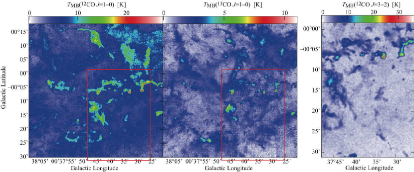
Figure 2: Peak intensity ($T_{\rm MB}$) maps of the ${}^{12}{\rm CO}$ $J=1\mbox{--}0$, ${}^{13}{\rm CO}$ $J=1\mbox{--}0$, and ${}^{12}{\rm CO}$ $J=3\mbox{--}2$ lines. The region in which the ${}^{12}{\rm CO}$ $J=3\mbox{--}2$ line was observed is indicated by red rectangles in the $J=1\mbox{--}0$ maps.

The ${}^{12}{\rm CO}\;J=3\mbox{--}2$ data (Sawada et al. in prep.) are compared with the $J=1\mbox{--}0$ lines. The observations of the $J=3\mbox{--}2$ line were made with the Atacama Submillimeter Telescope Experiment (ASTE) 10-m telescope at Pampa la Bola, Chile (Ezawa et al., 2004; Kohno, 2005) in September 2005. The region of $37\fdg 43\lesssim l\lesssim 37\fdg 80$, $-0\fdg 52\lesssim b\lesssim+0\fdg 02$ (a part of the 45-m field of view: see Fig. 2) was mapped using the OTF technique. The HPBW and $\eta_{\rm MB}$ of the telescope were $22\arcsec$ and 0.6, respectively. The data were reduced with NOSTAR and the reduced data cube has an effective resolution of $24\arcsec\times 24\arcsec\times 0.87\;{\rm km\;s^{-1}}$. Details will be described in a forthcoming paper. The peak intensity maps of the three lines are presented in Fig. 2.

4 Results and Discussion

4.1 Velocity Channel Maps

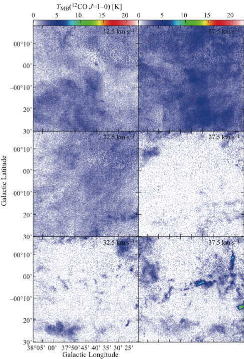
Figure 3: Velocity channel maps of ${}^{12}{\rm CO}$ $J=1\mbox{--}0$ $T_{\rm MB}$. The centroid velocity of each 5-${\rm km\;s^{-1}}$ channel is shown at the top-right corner.

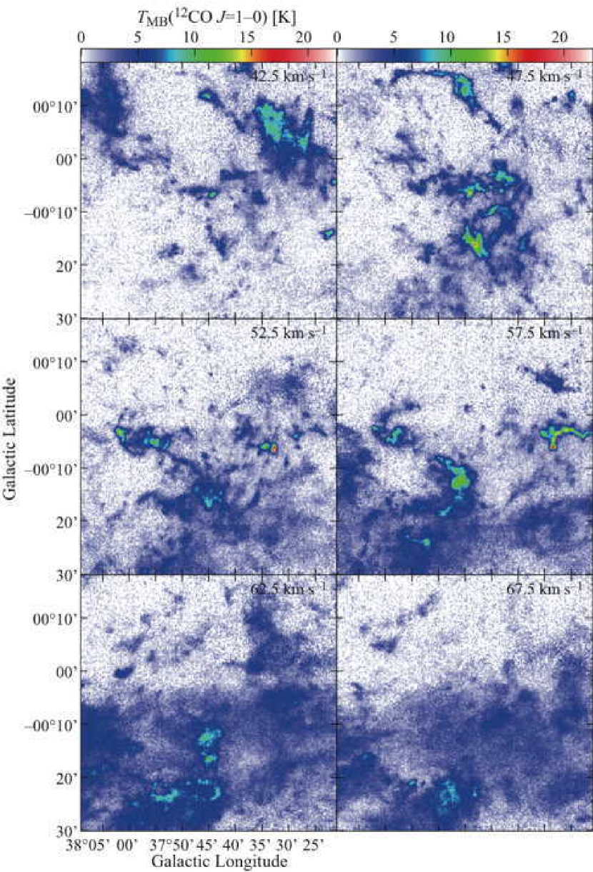
Figure 3: Continued

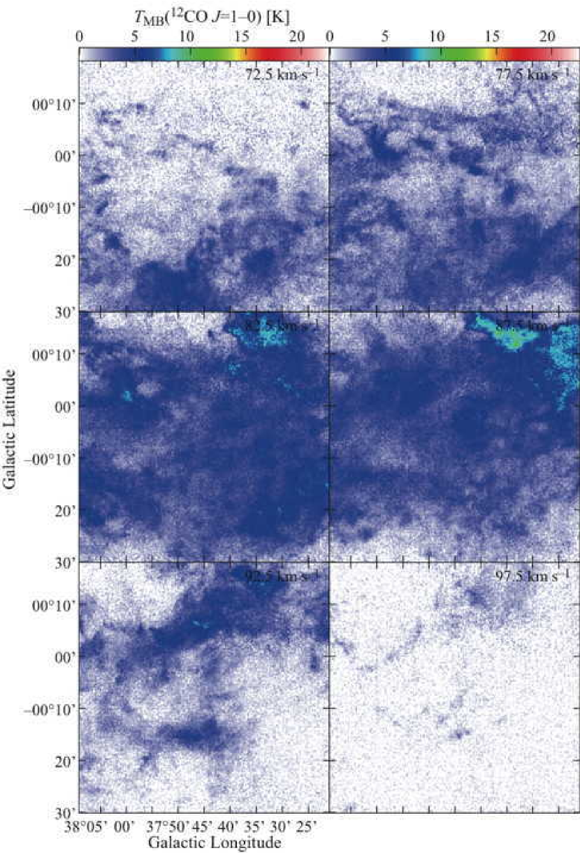
Figure 3: Continued

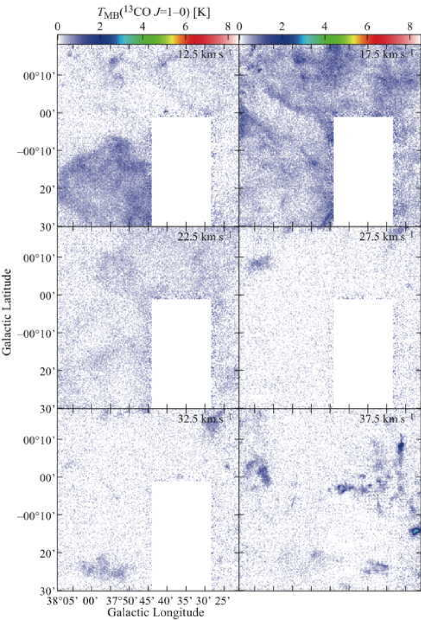
Figure 4: Same as Fig. 3, but for the ${}^{13}{\rm CO}$ $J=1\mbox{--}0$ line.

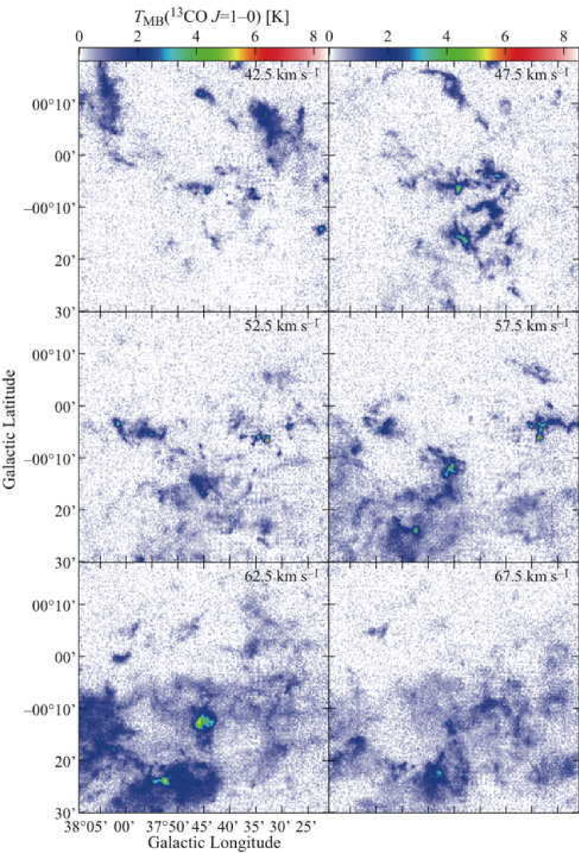
Figure 4: Continued

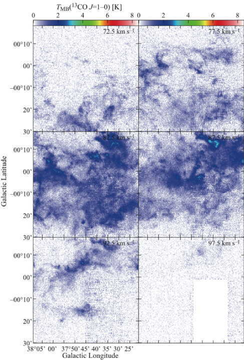
Figure 4: Continued

Figs. 3 and 4 show the velocity channel maps of the ${}^{12}{\rm CO}$ and ${}^{13}{\rm CO}$ lines, respectively, which cover the velocity range $v_{\rm LSR}=10\mbox{--}100\;{\rm km\;s^{-1}}$ with an interval of 5 ${\rm km\;s^{-1}}$.

The distribution of the emission in the channel maps significantly changes with the velocity. At the lowest velocity (10–25 ${\rm km\;s^{-1}}$) in Fig. 3, low brightness ${}^{12}{\rm CO}$ emission originating in the solar neighborhood is widespread in the field of view. Beyond 25 ${\rm km\;s^{-1}}$, the widespread emission vanishes. Instead, bright ($T_{\rm MB}\gtrsim 10\;{\rm K}$) and spatially confined structures begin to dominate at $\gtrsim 35\;{\rm km\;s^{-1}}$. These structures have sharp boundaries and form clumps (e.g., at $l\simeq 37\fdg 5$, $b\simeq-0\fdg 1$, $v_{\rm LSR}=52.5\;{\rm km\;s^{-1}}$) and filaments (e.g., at the top of the panel at 47.5 ${\rm km\;s^{-1}}$). Beyond $\gtrsim 60\;{\rm km\;s^{-1}}$, the bright structures become less prominent. Though they remain up to 62.5 ${\rm km\;s^{-1}}$ (at the bottom of the panel), low brightness extended emission starts to spread over the field. At the tangent velocity (75–90 ${\rm km\;s^{-1}}$), the low brightness ($\simeq 4\;{\rm K}$) emission almost fills the field of view, except a lump of $\simeq 10\;{\rm K}$ emission at the top-right corner of the field. The high surface filling factor at the tangent velocity can be attributed partly to the velocity crowding effect; nevertheless, the lack of bright structures is a distinct difference from the velocity range of 40–60 ${\rm km\;s^{-1}}$ (Section 4.2).

The ${}^{13}{\rm CO}$ channel maps (Fig. 4) show similar characteristics as those seen in the ${}^{12}{\rm CO}$ maps: the bright ($\gtrsim 4\;{\rm K}$), compact structures dominate at 40–65 ${\rm km\;s^{-1}}$, whereas the emission of 1–2 K is widespread at 75–90 ${\rm km\;s^{-1}}$. The ${}^{13}{\rm CO}$ maps have, in general, higher brightness contrast than those of the ${}^{12}{\rm CO}$ line, likely due to the lower optical depth. One of the most extreme cases is the 62.5-${\rm km\;s^{-1}}$ channel. The bright ($\gtrsim 4\;{\rm K}$) clumps seen in the ${}^{13}{\rm CO}$ map are not very prominent in ${}^{12}{\rm CO}$, implying the gas in the foreground with low excitation temperature obscures the bright ${}^{12}{\rm CO}$ line of the clumps.

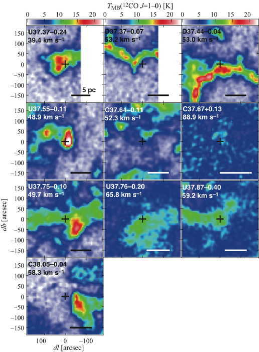
Figure 5: The ${}^{12}{\rm CO}\;J=1\mbox{--}0$ peak intensity ($T_{\rm MB}$) maps around the H II regions (shown as crosses) in Anderson & Bania (2009). The velocity range is $\pm 5\;{\rm km\;s^{-1}}$ from the radial velocity of the H II region, which is shown in each panel. The horizontal bars indicate the linear scale of 5 pc. Note that the coordinates in the catalog are given to the second decimal place in degrees: the sizes of the crosses are $\pm 0\fdg 005$ representing the uncertainty of the position.

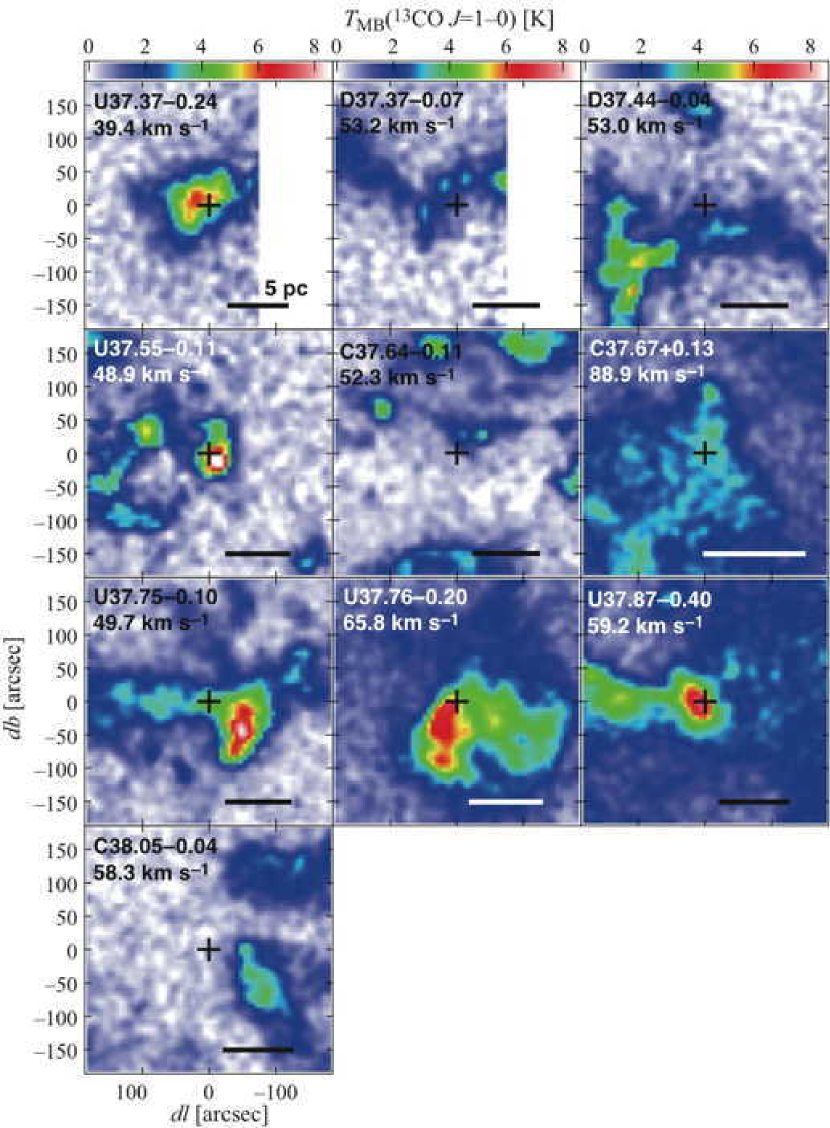
Figure 6: Same as Fig. 5, but for ${}^{13}{\rm CO}$.

Anderson & Bania (2009) compiled catalogues of H II regions in the first Galactic quadrant, and determined the distances to them, resolving the near-far distance ambiguity using the H I emission/absorption method and the H I self-absorption method. Their catalog contains 10 H II regions situated in our field of view (Table 2). Figs. 5 and 6 show the peak brightness maps around the H II regions in ${}^{12}{\rm CO}$ and ${}^{13}{\rm CO}$, respectively. Nine of them are associated with the bright ($>10\;{\rm K}$ in ${}^{12}{\rm CO}$ and/or $>4\;{\rm K}$ in ${}^{13}{\rm CO}$) clumps or filaments within a few pc. In particular, 5 ultracompact H II regions (whose names begin with ‘U’) are all tightly associated with the molecular clumps. This is consistent with Anderson et al. (2009). One exception is C37.67$+$0.13 at the tangent velocity. The ${}^{12}{\rm CO}$ around this object appears weak and extended, probably due to the self-absorption. The ${}^{13}{\rm CO}$ line is rather faint ($\approx 4\;{\rm K}$) in comparison with the other regions.

Our sufficient ($\lesssim 1\;{\rm pc}$) spatial resolution reveals that the spatial structure of molecular gas varies with the radial velocity and thus with respect to the Galactic structure. We classify the structures into the following two components, the B component and the D component. The B component is bright ($T_{\rm MB}>10\;{\rm K}$ in ${}^{12}{\rm CO}$; $>4\;{\rm K}$ in ${}^{13}{\rm CO}$) and spatially confined emission. It appears as clumps and filaments in the channel maps, whose typical size and mass are $1\arcmin$–$3\arcmin$ (3–8 pc at 9 kpc) and $10^{3}$–$10^{4}M_{\sun}$, respectively. The D component is diffuse (i.e., spatially extended) and fainter ($T_{\rm MB}\simeq 4\;{\rm K}$ in ${}^{12}{\rm CO}$ and $\simeq 1\;{\rm K}$ in ${}^{13}{\rm CO}$) emission. The former is seen in the velocity range of $\simeq 40\mbox{--}60\;{\rm km\;s^{-1}}$, while the latter dominates the solar neighborhood (10–25 ${\rm km\;s^{-1}}$) and at the tangent velocity (75–90 ${\rm km\;s^{-1}}$). The emission in the range 60–65 ${\rm km\;s^{-1}}$ is in-between — possibly a transition between or the mixture of them.

A number of studies have been performed in order to investigate the distribution and physical conditions of the gas in the Milky Way Galaxy. Most of them started from the decomposition of emission into individual, discrete molecular clouds/clumps and determined their properties (see Section 1). For example, Scoville et al. (1987) identified 1427 clouds and 255 hot cloud cores from the Massachusetts-Stony Brook Survey data. Among them 19 and 1 are in our field of view, respectively. Their only hot cloud core is at $(l,b,v)=(37\fdg 55,-0\fdg 10,53\;{\rm km\;s^{-1}})$ and is a prototype of the B component in our classification. Our higher-resolution and Nyquist-sampled maps reveal a number of comparable structures (e.g., Fig. 2). We also find a significant extended molecular emission. The previous studies might have missed a considerable amount of emission because of the cloud identification, i.e., the assumption that the molecular gas forms discrete objects. The emission below the cloud boundary threshold can be inevitably excluded from such analyses. The D component has a typical intensity ($\simeq 4\;{\rm K}$) comparable to the boundary used by Scoville et al. (1987) and Solomon et al. (1987). Thus a significant fraction of emission would have been overlooked in their work. In our data, 62% and 48% of the ${}^{12}{\rm CO}$ emission is below 4 K in the velocity ranges of 40–60 and 75–90 ${\rm km\;s^{-1}}$, respectively. Though the B component emission will easily be identified as clouds/clumps, it only accounts for a small fraction of the total gas mass (Section 4.3). In the following, we address the characteristics of the gas in a quantitative fashion by using the crude observed line brightness, rather than extracting clouds.

4.2 Brightness Distribution Function

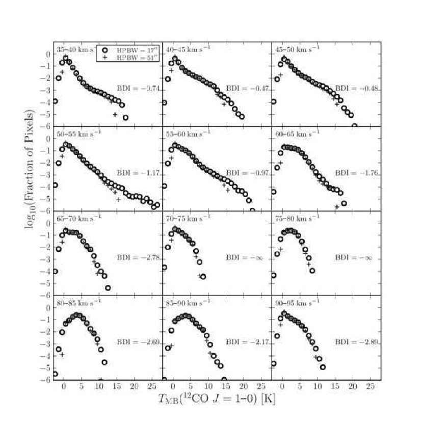
Figure 7: Histogram of the ${}^{12}{\rm CO}$ brightness temperature. The horizontal axis is the brightness temperature $T_{\rm MB}$ [K], and the vertical axis is the fraction of pixels in each 1-K brightness bin. Open circles and crosses represent the original resolution ($\mbox{effective HPBW}=17\arcsec$) and 3-times smoothed ($51\arcsec$) data, respectively.

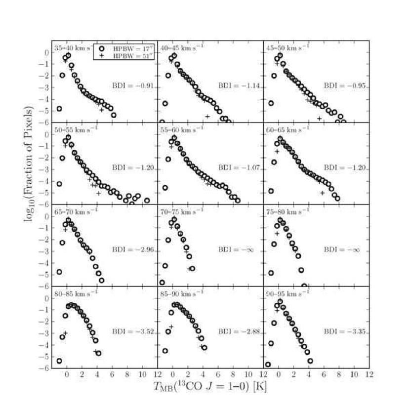
Figure 8: Same as Fig. 8, but for ${}^{13}{\rm CO}$. The width of each brightness bin is 0.4 K.

There is clear variation of spatial structure of the gas with the radial velocity. Here we use histograms of the brightness temperatures, or the Brightness Distribution Functions (BDFs), which visualize the spatial structure of the gas without separating structures into arbitrary clouds. Figs. 7 and 8 present the BDFs of ${}^{12}{\rm CO}$ and ${}^{13}{\rm CO}$, respectively. The data with the $6\arcsec\times 6\arcsec\times 1.25\;{\rm km\;s^{-1}}$ grid are divided into 5-${\rm km\;s^{-1}}$ velocity channels, and the number of $l$-$b$-$v$ pixels in each 1 K (${}^{12}{\rm CO}$) and 0.4 K (${}^{13}{\rm CO}$) brightness bin is plotted (normalized by the total number of pixels in each velocity channel). In each panel the Brightness Distribution Index is also shown, which we introduce in the following subsection in order to quantify the characteristics of BDF.

The BDF clearly reflects the amount of the two components of molecular gas described above. The ${}^{12}{\rm CO}$ BDF in the $v_{\rm LSR}=35\mbox{--}40\;{\rm km\;s^{-1}}$ channel (Fig. 7) shows a sharp peak in the 0–1 K brightness bin. This corresponds to the fact that a large portion of the field of view is almost emission-free (Fig. 3). The high-brightness tail represents the B component in the right-hand side of the field (the most prominent structure is at $l=37\arcdeg 23\arcmin$, $b=-0\arcdeg 14\arcmin$). As the velocity goes up to $v_{\rm LSR}\approx 55\;{\rm km\;s^{-1}}$, the high-brightness tail is even more populated, and the peak brightness also increases. It corresponds to the B component structures in the velocity channel maps, with increased numbers (i.e., surface filling factors) and peak brightness. The peak of the BDF at $\simeq 0\;{\rm K}$ is still prominent, reflecting the relatively small surface filling factor of the CO emission. At $\approx 60\;{\rm km\;s^{-1}}$, the 0-K peak starts to drop, and another remarkable component, the shoulder at $\approx 4\;{\rm K}$, emerges. It reflects the D component which fills the bottom half of the field. At $\approx 75\;{\rm km\;s^{-1}}$, the high-brightness tail truncates, while the 4-K shoulder still exists. At the tangent velocity (75–90 ${\rm km\;s^{-1}}$), the 0-K peak is no longer prominent, and the 4-K shoulder turns into a peak. This transition is obvious in the channel maps, in which D component fills almost the whole field of view. Beyond 95 ${\rm km\;s^{-1}}$, the 0-K peak reappears since the surface filling factor of the D component decreases. The BDF, with a 4-K shoulder and truncation toward high brightness, is similar to that at 65–75 ${\rm km\;s^{-1}}$.

The ${}^{13}{\rm CO}$ BDF shows a similar trend — high-brightness ($\gtrsim 4\;{\rm K}$) tail at 40–65 ${\rm km\;s^{-1}}$, truncation beyond 65 ${\rm km\;s^{-1}}$, and a shoulder at $\approx 1\;{\rm K}$ at the tangent velocity. The ${}^{13}{\rm CO}$ BDF has, in general, a more prominent 0-K peak and sharper truncation toward the high-brightness tail, which come from the higher brightness contrast in the ${}^{13}{\rm CO}$ channel maps (Section 4.1).

We suggest that the difference of the BDF between the Sgr arm ($40\mbox{--}60\;{\rm km\;s^{-1}}$) and the inter-arm region ($75\mbox{--}90\;{\rm km\;s^{-1}}$) is due to a change of gas properties. There are, however, a couple of potential issues that we should consider, which might cause apparent variation between the velocity components: (a) distance from us (i.e., linear resolution), and (b) velocity crowding.

In order to test (a), we convolve the maps with a Gaussian to degrade the resolution by a factor of 3 (equivalent to ${\rm HPBW}=51\arcsec$) and see how the spatial resolution affects the map’s appearance and thus the BDF. The BDFs from the convolved maps (crosses in Figs. 7 and 8) confirm the features discussed above. This implies that a near-far distance ambiguity up to a factor of $\approx 3$ (Section 2) does not affect the result.

As for (b), the line-of-sight path length in a 10-${\rm km\;s^{-1}}$ bin for the tangent component is $\approx 2.5$ times larger than those for the near- and far-side Sgr arm (Section 2). This increases the $(l,b,v)$-volume filling factor of the emitting region in the tangent component, which may have turned the 4-K shoulder in the ${}^{12}{\rm CO}$ BDF into the peak seen at the tangent velocity. The absence of bright ($\gtrsim 10\;{\rm K}$) ${}^{12}{\rm CO}$ emission may possibly be attributed to velocity crowding and self-absorption. However, the optically thin ${}^{13}{\rm CO}$ emission also lacks bright ($\gtrsim 4\;{\rm K}$) structures at this velocity. This supports that the BDF in the inter-arm region differs intrinsically from that in the Sgr arm.

4.3 Brightness Distribution Index

The BDFs clearly characterize the variation of the spatial structure, showing the bright, compact clumps/filaments and more extended component of molecular gas. We introduce the brightness distribution index (BDI) to characterize the BDF with one number, which can be correlated with other parameters, such as the physical conditions of the gas and star-forming activity. The BDI is defined as the flux ratio of the bright emission to the low-brightness emission:

$${\mit BDI} = \log_{10}\left(\frac{\int_{T_{2}}^{T_{3}}T\cdot B(T)dT}{\int_{T_{0}}^{T_{1}}T\cdot B(T)dT}\right)$$ (1)

$$= \log_{10}\left(\frac{\sum_{T_{2}<T[i]<T_{3}}T[i]}{\sum_{T_{0}<T[i]<T_{1}}T[i]}\right),$$

where the BDF is denoted as $B(T)$; $T_{0}$, $T_{1}$, $T_{2}$, and $T_{3}$ are the brightness thresholds; and $T[i]$ is the brightness of the $i$-th pixel. We note that the flux is roughly proportional to the mass.

In this paper we adopt $(T_{0},T_{1},T_{2},T_{3})=(3,5,10,\infty)$ for ${}^{12}{\rm CO}$ and $(1,1.5,4,\infty)$ for ${}^{13}{\rm CO}$. These thresholds are somewhat arbitrary, but are empirically chosen so that the numerator and the denominator of Eq. (1) represent the gas of the typical brightness of the B and D components that are evident in the channel maps (Section 4.2), respectively. The typical molecular gas temperature that is determined in a wider Galactic plane ${}^{12}{\rm CO}$ survey is $\simeq 10$ K (Scoville & Sanders, 1987); subtracting the cosmic microwave background temperature, the average brightness temperature would be $\simeq 7$ K. Our choice of the thresholds represents the brightness appreciably below and above this average over the large area in the Galactic plane. The thresholds for ${}^{13}{\rm CO}$ are adjusted correspondingly to pick out the similar regions in the maps (Figs. 3 and 4). In the following we demonstrate the utility of the BDI to characterize the spatial structure, despite that the thresholds can be specific to the line of sight we observed. An important future work is to revisit the choice of these parameters when more examples become available.

The BDIs for ${}^{12}{\rm CO}$ and ${}^{13}{\rm CO}$ within the 5-${\rm km\;s^{-1}}$ velocity bins are shown in Figs. 7 and 8, respectively. At $v_{\rm LSR}\simeq 40\mbox{--}60\;{\rm km\;s^{-1}}$ the BDIs are higher ($-1.2$–$-0.5$ in ${}^{12}{\rm CO}$, $-1.2$–$-0.9$ in ${}^{13}{\rm CO}$), while at the $80\mbox{--}90\;{\rm km\;s^{-1}}$ BDIs are lower ($-2.7$–$-2.2$ in ${}^{12}{\rm CO}$, $-3.5$–$-2.9$ in ${}^{13}{\rm CO}$). The fraction of bright emission varies with velocity. It is also remarkable that even at the velocities with a high BDI (i.e., in spiral arm), only a small fraction of the gas is composed in the B component. That is, despite the highest ${}^{12}{\rm CO}$ BDI ($-0.47$) at 45–50 ${\rm km\;s^{-1}}$, the flux of the $T_{\rm MB}>T_{2}$ emission amounts to only one third of the $T_{0}<T_{\rm MB}<T_{1}$ emission, or, 6.6% of the total flux. The mass fraction of the B component gas is even lower at other radial velocities.

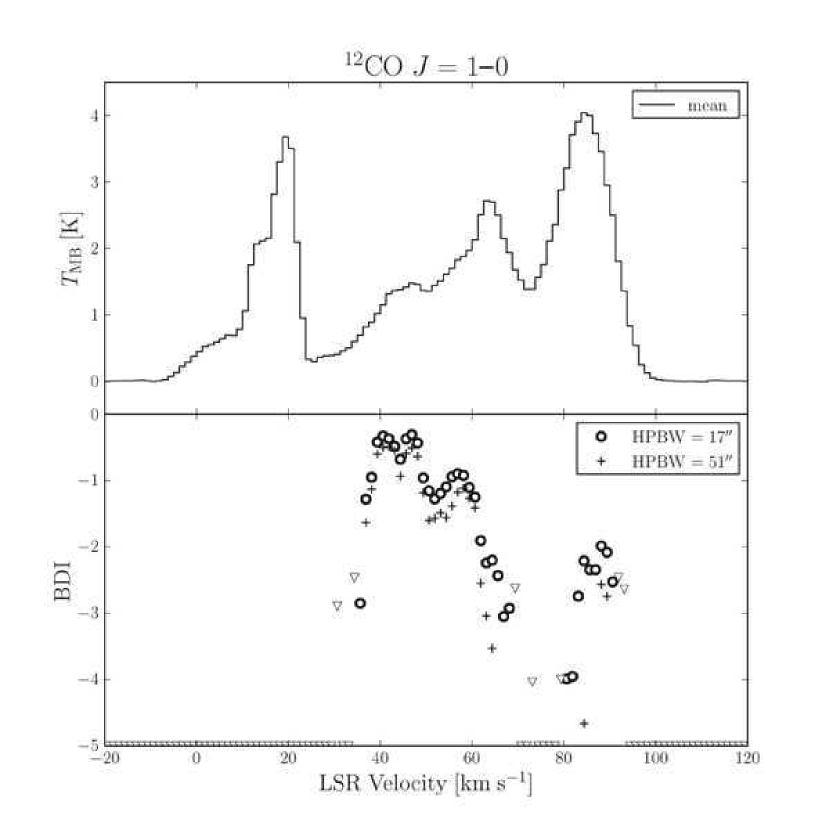
Figure 9: (Top) The mean brightness of the ${}^{12}{\rm CO}$ line. (Bottom) The velocity profile of the BDI. Open circles and crosses represent the original resolution and 3-times smoothed data, respectively. Open triangles are the upper limit of the BDI, defined as $\log_{10}\{{\sum_{T_{2}<(T[i]+3\sigma)}(T[i]+3\sigma)}/{\sum_{T_{0}<T[i]<T_{1}}T[i]}\}$ ($\sigma$ is the RMS noise of the map), for the original resolution data.

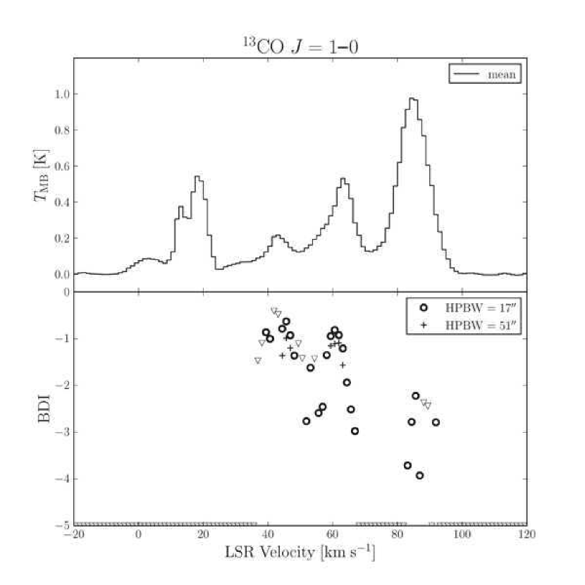
Figure 10: Same as Fig. 9, but for ${}^{13}{\rm CO}$. The region observed in Period 1 is excluded since the velocity coverage is narrow.

The variation of BDI as a function of radial velocity (i.e., velocity profiles of BDIs) for ${}^{12}{\rm CO}$ and ${}^{13}{\rm CO}$ are presented in Figs. 9 and 10, along with the mean brightness in the field. The line brightness shows 4 prominent peaks at $20\;{\rm km\;s^{-1}}$ (solar neighborhood), $45\;{\rm km\;s^{-1}}$ (near-side Sgr arm), $65\;{\rm km\;s^{-1}}$ (far-side Sgr arm), and $85\;{\rm km\;s^{-1}}$ (tangent velocity). The BDI in ${}^{12}{\rm CO}$ is high in the velocity range 40–60 ${\rm km\;s^{-1}}$ (i.e., Sgr arm), with a steep decrease beyond 60 ${\rm km\;s^{-1}}$. The BDI is low at 80–90 ${\rm km\;s^{-1}}$. In other velocity ranges the BDI is infinitely small because of the lack of $\geq T_{2}$ emission. The ${}^{13}{\rm CO}$ BDI behaves similarly to that of ${}^{12}{\rm CO}$: it is high in 40–60 ${\rm km\;s^{-1}}$ with peaks at 45 and 60 ${\rm km\;s^{-1}}$ (the Sgr arm), and is low in 80–90 ${\rm km\;s^{-1}}$ (the inter-arm region). Molecular gas is extended with little brightness variation in the inter-arm region, and bright, compact structures emerge in spiral arms.

4.4 Comparison with CO Intensity Ratios

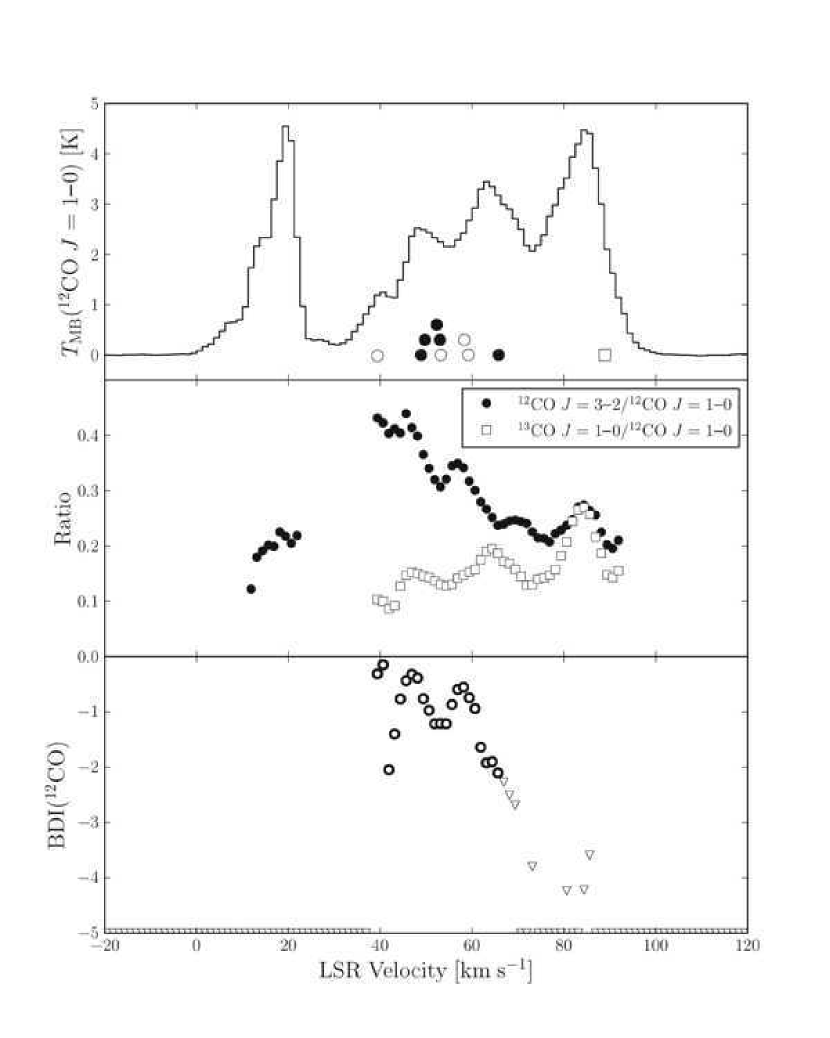
Figure 11: (Top) The line profile of ${}^{12}{\rm CO}\;J=1\mbox{--}0$. The radial velocities of the H II regions taken from Anderson & Bania (2009) are also shown as circles (at the far side), and a square (at the tangent point). The H II regions inside the ASTE field of view are drawn as filled symbols, while the others are open. (Middle) The ${}^{12}{\rm CO}\;J=3\mbox{--}2/^{12}{\rm CO}\;J=1\mbox{--}0$ and ${}^{13}{\rm CO}\;J=1\mbox{--}0/^{12}{\rm CO}\;J=1\mbox{--}0$ intensity ratios. Note that the ${}^{12}{\rm CO}\;J=3\mbox{--}2/^{12}{\rm CO}\;J=1\mbox{--}0$ ratio is most probably underestimated (see text). (Bottom) The BDI in ${}^{12}{\rm CO}\;J=1\mbox{--}0$, inside the region $37\fdg 43\lesssim l\lesssim 37\fdg 80$, $-0\fdg 50\lesssim b\lesssim+0\fdg 02$.

The ${}^{12}{\rm CO}\;J=3\mbox{--}2$ data are available for a smaller field (Fig. 2), $\approx 1/4$ of the 45-m field of view. The BDI, the ${}^{12}{\rm CO}\;J=1\mbox{--}0$ brightness, the $T_{\rm MB}(^{12}{\rm CO}\;J=3\mbox{--}2)/T_{\rm MB}(^{12}{\rm CO}\;J=1\mbox{--}0)$ ratio [$R_{3\mbox{--}2/1\mbox{--}0}(^{12}{\rm CO})$], and the $T_{\rm MB}(^{13}{\rm CO}\;J=1\mbox{--}0)/T_{\rm MB}(^{12}{\rm CO}\;J=1\mbox{--}0)$ ratio [$R_{13/12}(J=1\mbox{--}0)$] are shown in Fig. 11. The overall characteristics of the ${}^{12}{\rm CO}$ brightness and the BDI are similar to those in the whole 45-m field of view (Fig. 9). The $R_{3\mbox{--}2/1\mbox{--}0}(^{12}{\rm CO})$ is the highest at the radial velocity of 40–45 ${\rm km\;s^{-1}}$ and tends to decrease toward the higher velocity. It has local peaks at 40–45, 55, and 85 ${\rm km\;s^{-1}}$. The first two peaks agree with those of the BDI. If we assume that the brightness peaks at $\approx 47$ and 63 ${\rm km\;s^{-1}}$ trace the near- and far-side Sgr arm respectively, these BDI and $R_{3\mbox{--}2/1\mbox{--}0}(^{12}{\rm CO})$ peaks are both offset from the corresponding brightness peaks toward the lower velocity by several ${\rm km\;s^{-1}}$ (discussed in Section 4.6). On the other hand, the radial velocity of the third peak coincides with that of the brightness peak. The $R_{13/12}(J=1\mbox{--}0)$ generally correlates with the brightness, and traces the optical depth (the column density) of the gas. Thus the ${}^{12}{\rm CO}$ brightness peaks correspond to the peaks of molecular gas distribution along the radial velocity.

The sets of the ratios $(R_{3\mbox{--}2/1\mbox{--}0}(^{12}{\rm CO}),R_{13/12}(J=1\mbox{--}0))$ are calculated for the two components (1) $v_{\rm LSR}=40\mbox{--}60\;{\rm km\;s^{-1}}$, $T_{\rm MB}(^{12}{\rm CO})>10\;{\rm K}$ and (2) $v_{\rm LSR}=70\mbox{--}80\;{\rm km\;s^{-1}}$, $T_{\rm MB}(^{12}{\rm CO})=3\mbox{--}5\;{\rm K}$. They represent the B and D components. The ratios are derived as $(\geq 0.63\pm 0.03,0.23\pm 0.02)$ and $(0.40\pm 0.11,0.16\pm 0.05)$, respectively. The errors quoted are estimated from baseline uncertainties (i.e., constant offset of $1\sigma$ is assumed in all spectra over all channels, which we consider as a very conservative estimate) and the random noise.

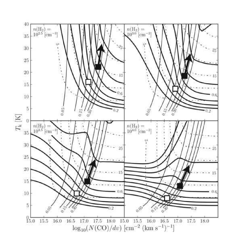
Figure 12: The LVG results for $n({\rm H_{2}})=10^{2.5}$, $10^{3.0}$, $10^{3.5}$, and $10^{4.0}\;{\rm cm^{-3}}$. The $R_{3\mbox{--}2/1\mbox{--}0}(^{12}{\rm CO})$, $R_{13/12}(J=1\mbox{--}0)$, and the ${}^{12}{\rm CO}\;J=1\mbox{--}0$ brightness temperature are drawn as thick solid lines (the contour levels are 0.2, 0.3, 0.4, …), thin solid lines (0.05, 0.10, 0.15, …), and dashed lines (5, 10, 15, … [K]), respectively. Estimated physical conditions for the two components (B component and D component) are marked as the filled and open squares.

In order to estimate qualitatively what the main difference between the two component is, we compare the obtained intensity ratios with simple model calculations. Here we use the large-velocity-gradient (LVG; Goldreich & Kwan, 1974; Scoville & Solomon, 1974) model and adopt the one-zone assumption: i.e., the emission lines originate in a homogeneous volume of the gas. More detailed analyses of the physical conditions of the gas by using more lines will be reported in a forthcoming paper. Fig. 12 shows the result of LVG calculations made with RADEX (van der Tak et al., 2007). The $R_{3\mbox{--}2/1\mbox{--}0}(^{12}{\rm CO})$, $R_{13/12}(J=1\mbox{--}0)$, and the ${}^{12}{\rm CO}\;J=1\mbox{--}0$ brightness temperature were calculated as functions of the kinetic temperature of the gas ($T_{\rm k}$) and the column density of ${}^{12}{\rm CO}$ molecules per unit velocity width [$N({\rm CO})/dv$]. The number density of molecular hydrogen [$n({\rm H_{2}})$] was assumed to be $10^{2.5}$, $10^{3.0}$, $10^{3.5}$, and $10^{4.0}$ ${\rm cm^{-3}}$. The ${}^{12}{\rm C}/^{13}{\rm C}$ abundance ratio at a Galactocentric distance of 6 kpc was estimated to be 40–55 (Langer & Penzias, 1993; Savage et al., 2002; Milam et al., 2005). Here we adopted 50 for the calculation. The physical conditions which reproduce the observed intensity ratios are plotted as the filled and open squares. The $T_{\rm k}$ of the two components are estimated to be $\geq 13\mbox{--}22$ and 8–16 K if the $n({\rm H_{2}})$ is in the range of $10^{2.5}\mbox{--}10^{4.0}\;{\rm cm^{-3}}$ (note that $R_{3\mbox{--}2/1\mbox{--}0}(^{12}{\rm CO})$, and thus the derived $T_{\rm k}$, of the B component gas is a lower limit). The gas in the B component is found to be warmer than that of the D component, as expected. Although no tight constraints on the gas density can be given, the possibility of the high ($n({\rm H_{2}})\gtrsim 10^{4}\;{\rm cm^{-3}}$) density of the D component is rejected because the observed brightness cannot be reproduced even if the surface filling factor is unity.

4.5 Comparison with H II Regions

The H II region catalog compiled by Anderson & Bania (2009) contains 10 samples in our field of view (Table 2: see Section 4.1). The radial velocities of these H II regions are plotted in Fig. 11. The ones in the ASTE field of view are shown in filled symbols, while the others are open. Eight H II regions are located at the far side (circles in Fig. 11, top), and they are mostly concentrated at $\approx 50\mbox{--}60\;{\rm km\;s^{-1}}$. This coincides with the velocity range where the BDI and the $R_{3\mbox{--}2/1\mbox{--}0}(^{12}{\rm CO})$ are high.

These 8 H II regions at the far side ($50\mbox{--}60\;{\rm km\;s^{-1}}$) are most likely associated with the far-side Sgr arm (i.e., the peak of the brightness at $\approx 63\;{\rm km\;s^{-1}}$). Thus the H II regions in our line of sight have radial velocities systematically lower than that of the molecular spiral arm. We note again that the radial velocities of the BDI and $R_{3\mbox{--}2/1\mbox{--}0}(^{12}{\rm CO})$ peaks are offset from those of the CO brightness maxima toward the lower velocity (Section 4.4). All BDI and $R_{3\mbox{--}2/1\mbox{--}0}(^{12}{\rm CO})$ peaks and H II regions are offset in velocity from the spiral arm.

4.6 Molecular Gas and Spiral Arm

We identified two distinct components of the molecular gas, the B component and the D component, based on high-resolution, wide-field mapping observations of the Galactic plane. The B component emission is prominent at the velocities of the spiral arms, although its flux (mass) fraction of the total flux is small. The D component (and even fainter emission) is the majority of the molecular mass, dominating the emission both at the spiral arm and at the inter-arm velocities. We have introduced the BDF and the BDI to quantify the difference, and demonstrated that the BDI characterizes the structural variation of the gas along the line of sight: i.e., the BDI is high in the spiral arm velocities and low outside. The B component emission corresponds to the “warm” or “hot” clouds defined in Solomon, Sanders, & Rivolo (1985) and Scoville et al. (1987). Our analysis confirms their results that the “warm” or “hot” clouds are concentrated on the $l$-$v$ loci of the spiral arms and resolves them as bright clumps and filaments. The advantages of our study are the following: The high-resolution observations revealed that the D component emission is faint and spatially extended, and therefore was missed in the “cloud identification” scheme. This component consists about half the mass in our field and is quite substantial. Our method is free from the process of cloud identification and takes into account such a component as well as bright and clumpy (the B component) emission. Furthermore, the new parameter, BDI, characterizes the gas structure and is directly comparable with other tracers of the spiral arms (e.g., H II regions) and the physical conditions of the gas (e.g., line ratios).

Extended emission in CO $J=1\mbox{--}0$ has been found in external galaxies, especially in their inter-arm regions (e.g., Adler et al., 1992; Koda et al., 2009). However, at their current resolutions even with interferometers ($>100$ pc), it remains unclear if these components are an ensemble of small unresolved giant molecular clouds or truly-extended emission. Our results are drawn at a very high spatial resolution of $\simeq 0.5$ pc, and are therefore different from the extragalactic results both qualitatively and quantitatively. The relation between such small structures and kpc-scale galactic structures that we find in Figs. 3 and 4 is the new finding. The Atacama Large Millimeter/submillimeter Array will bridge the gap between these studies with its ability to produce high-fidelity images of pc-sized structures over nearby galaxies.

The peaks of the BDI coincide in velocity with the $R_{3\mbox{--}2/1\mbox{--}0}(^{12}{\rm CO})$ local maxima. The B component gas, which makes the BDI high, shows a high $R_{3\mbox{--}2/1\mbox{--}0}(^{12}{\rm CO})$ ratio and is warm, as opposed to the D component gas. The BDI peaks also coincide with H II regions, but are offset toward lower velocities from the maxima of the CO brightness (the near- and far-side Sgr arm). These results indicate that the distribution of the high-BDI gas and H II regions is shifted from the molecular spiral arm by several ${\rm km\;s^{-1}}$.

The offset in velocity between the high-BDI gas and molecular spiral arm implies that the high-BDI gas is located in the outer (i.e., larger Galactocentric radius: see Fig. 1b) side of the spiral arm. If we assume the 220-${\rm km\;s^{-1}}$ flat rotation of the Galaxy, the velocity offset (several ${\rm km\;s^{-1}}$) translates to $\simeq 500\;{\rm pc}$ in space. The corotation radius of spiral arms in the Milky Way Galaxy is likely outside the solar circle. Therefore the gas at a Galactocentric radius of 6 kpc revolves faster than the spiral pattern, by $\approx 100\;{\rm km\;s^{-1}}$. Hence, the gas with high BDI and high $R_{3\mbox{--}2/1\mbox{--}0}(^{12}{\rm CO})$ and star-forming regions are located on the downstream side of the spiral arm (CO brightness peak) in our field of view. If we assume a pitch angle of the Sgr arm of $12\arcdeg$ (Georgelin & Georgelin, 1976), the drift timescale for the offset is $\sim 20\;{\rm Myr}$. This is consistent with the timescale found in other galaxies (Egusa et al., 2009). Note that the velocity offset may partially be attributed to the effect of radiative transfer (e.g., the B component gas in the spiral arm velocity with high $R_{3\mbox{--}2/1\mbox{--}0}(^{12}{\rm CO})$ may be obscured by the bulk D component gas) and needs to be verified by using optically thinner lines. Nevertheless, the asymmetry of BDI, $R_{3\mbox{--}2/1\mbox{--}0}(^{12}{\rm CO})$, and the distribution of H II regions with respect to the arm velocities indicates that the trend is real.

We treated the tangent-velocity gas as a prototype of the gas in the inter-arm region. There are, however, some caveats. First, this line of sight shows slightly more emission at the tangent velocity compared with the neighboring longitudes (e.g., Fig. 3 in Dame, Hartmann, & Thaddeus, 2001). This area is a molecular-rich inter-arm region. Second, the BDI is higher compared with the other velocity ranges corresponding to inter-arm regions: i.e., between the far-side Sgr arm and the tangent velocity (70–80 ${\rm km\;s^{-1}}$) and the solar neighborhood ($\simeq 20\;{\rm km\;s^{-1}}$). The emission at the tangent velocity has been proposed, though not proven, as a special structure, a spur that extends from a spiral arm into the inter-arm region (e.g., Dame et al., 1986). Sakamoto et al. (1997) found that there was no enhancement of the ${}^{12}{\rm CO}\;J=2\mbox{--}1/^{12}{\rm CO}\;J=1\mbox{--}0$ ratio and deduced a lower gas density than the average over a much larger region. Koda et al. (2009) performed high-resolution mapping observations of the ${}^{12}{\rm CO}\;J=1\mbox{--}0$ line in the entire disk of M51 and detected spurs in the inter-arm regions. The gas at our tangent velocity could be a relatively molecular-rich portion of the inter-arm region. Still, the clear difference of gas structure between spiral arms and inter-arm regions is striking. The richness of molecular gas is not the only determinant of gas structure. There is a correlation with large galactic structure.

5 Conclusions

We performed mapping observations of a $0\fdg 8\times 0\fdg 8$ field on the Galactic plane in the ${}^{12}{\rm CO}$ and ${}^{13}{\rm CO}$ $J=1\mbox{--}0$ lines. The high-resolution maps resolve the spatial structure of the emission down to $\lesssim 1\;{\rm pc}$ and clearly show its variation with the radial velocity, and therefore, between spiral arm and inter-arm regions. The bright and spatially confined emission (B component) is prominent in the Sgr arm, while the fainter, diffuse emission (D component) dominates in the inter-arm regions. We investigated the characteristics of the gas and revealed the followings:

• The typical size and mass of the B component structures are $1\arcmin\mbox{--}3\arcmin$ (3–8 pc at 9 kpc) and $10^{3}$–$10^{4}M_{\sun}$, respectively; and it contains only a small fraction of the total gas mass. The B component exists predominantly in spiral arms. The D component is widespread and dominant in the inter-arm region. It also exists in the arm as well.

• The BDFs characterize the variation of the spatial structure of the gas. We also defined a new parameter, BDI, as the flux ($\sim{\rm mass}$) ratio between the B component and D component, in order to characterize the spatial structure.

• High BDI coincides with high $R_{3\mbox{--}2/1\mbox{--}0}(^{12}{\rm CO})$. Thus the high BDI component contains warm/hot gas.

• High BDI also coincides with H II regions. Almost all H II regions are associated with the B component emission.

• The high-BDI gas (and thus, the high $R_{3\mbox{--}2/1\mbox{--}0}(^{12}{\rm CO})$ gas and star-forming regions) is offset from the peak of the line brightness toward lower velocities, i.e., the downstream side of molecular spiral arms. This implies that B component (warm gas) develops at the downstream side of the spiral arm and forms stars there.

These analyses are based on the pixel-by-pixel brightness distribution and are free from the process of cloud identification. Our method is advantageous in investigating the molecular gas content in the Galaxy as a whole, since the majority of the emission in our field of view is found as the diffuse, more extended component (D component), which does not come under the traditional “cloud” classification.

Appendix A Possible Deviation from the Assumed Structure of the Galaxy

Although we assumed the structure of the Galaxy briefly described in Section 2, the precise picture is the topic under debate. Georgelin & Georgelin (1976) referred to the Sgr and Sct arms as “major” and “intermediate” arms, on the basis of a study of H II regions. “Warm” or “hot” molecular clouds follow the $l$-$v$ loci of the H II regions in these arms (Solomon, Sanders, & Rivolo, 1985; Sanders et al., 1985; Scoville et al., 1987), as mentioned in Section 1. These studies suggested that the Sgr arm is a major and prominent arm. On the other hand, Drimmel (2000) presented that at the Sgr tangent ($l\simeq 50\arcdeg$) there is no enhancement in the K band, as opposed to the Sct tangent ($l\simeq 30\arcdeg$), and suggested that the Sgr is an interarm or secondary arm structure. Similar results were also achieved from mid-infrared star count (Benjamin et al., 2005; Churchwell et al., 2009).

In this paper we regarded the radial velocities at which the total CO intensity within the field of view takes its maxima as “spiral arm” velocities, and found that they coincide with the traditional Sgr arm velocities (e.g., Sanders et al., 1985). We then focused on the relationship between the indices of the gas properties (BDF/BDI, line ratios, and H II regions) and the arm velocities. Our study, therefore, relies on the existence of the Sgr arm and the assumption that the observed maxima of the total CO intensity correspond to the Sgr arm, but is independent of the details of the structure of the Galaxy (i.e., whether the Sgr arm is a major or secondary arm, and its exact location in the Galaxy). The location (distance) of the observed gas content is affected by the near-far distance ambiguity and the deviation from the flat, circular rotation of the Galaxy. The near-far ambiguity was taken into account in the analyses of the BDI and BDF and the difference between the arm and the inter-arm regions was proven to be firm. The implication that the high-BDI gas and H II regions are located in the outer side of the spiral arm (from the fact that they have lower radial velocities than the brightness peak) is unchanged regardless of the near-far ambiguity, unless the local non-circularity (streaming motion) overrides the global trend of the velocity field of the Galaxy.

Appendix B Systematic Errors in Intensity Ratios

The $T_{\rm MB}$ brightness scale is likely overestimated because the sources are, in general, bigger than the main beam sizes of the telescopes. In particular, $\eta_{\rm MB}$ of the 45-m telescope differs significantly from $\eta_{\rm moon}$, which means a considerable amount of power comes from the sidelobe. Since the emission in the velocity range of 70–80 ${\rm km\;s^{-1}}$ is widespread over the field of view, the coupling efficiency $\eta_{\rm c}$ should be close to $\eta_{\rm moon}$ rather than $\eta_{\rm MB}$. Therefore we adopt $\eta_{\rm c}\simeq\eta_{\rm moon}=0.69$ for this component. On the other hand, the high-brightness structures are less affected because of their low surface filling factors. The typical size of these structures is up to a few arcminutes (Section 4.1). The 45-m telescope, whose dish consists of 1- to 2-m reflection panels, is considered to have an error patterns of $5\arcmin\mbox{--}10\arcmin$ width. Thus a high-brightness structure fills only a small part of the error pattern: we use $\eta_{\rm MB}$ as the lower limit of $\eta_{\rm c}$. We consider that the error of the CO $J=3\mbox{--}2$ brightness due to the error pattern of the ASTE telescope is small compared with that of the $J=1\mbox{--}0$, given the high $\eta_{\rm MB}$ of the telescope.

Table 1: Parameters of the Observations and Reduced Maps

	Period 1		Period 2
	(2002 Nov – 2003 May)		(2005 Dec – 2006 Mar)
	${}^{13}{\rm CO}\;J=1\mbox{--}0$		${}^{12}{\rm CO}\;J=1\mbox{--}0$	${}^{13}{\rm CO}\;J=1\mbox{--}0$
Grid spacing	$13\farcs 7$ (PSW)		Nyquist (OTF)	Nyquist (OTF)
Area (${\mit\Delta}l\times{\mit\Delta}b$)	$0\fdg 3\times 0\fdg 5$		$0\fdg 8\times 0\fdg 8$	$0\fdg 8\times 0\fdg 8$
Bandwidth	32 MHz (87.0 ${\rm km\;s^{-1}}$)		512 MHz (1330 ${\rm km\;s^{-1}}$)	32 MHz (87.0 ${\rm km\;s^{-1}}$)
	$\cdots$		$\cdots$	512 MHz (1390 ${\rm km\;s^{-1}}$)
Frequency resolution	37.8 kHz (0.10 ${\rm km\;s^{-1}}$)		1 MHz (2.6 ${\rm km\;s^{-1}}$)	62.5 kHz (0.17 ${\rm km\;s^{-1}}$)
	$\cdots$		$\cdots$	1 MHz (2.7 ${\rm km\;s^{-1}}$)
Main-beam efficiency	$0.46\pm 0.03$		$0.39\pm 0.03$	$0.45\pm 0.03$
System noise temperature (DSB)	300–600 K		350–450 K	300–400 K
Map grid	$6\farcs 85$		$6\arcsec$	$6\arcsec$
Effective HPBW	$20\arcsec$		$17\arcsec$	$17\arcsec$
RMS noise ($T_{\rm MB}$)	0.57 K (at 0.2 ${\rm km\;s^{-1}}$)		0.44 K (at 2.6 ${\rm km\;s^{-1}}$)	0.62 K (at 0.2 ${\rm km\;s^{-1}}$)
	$\cdots$		$\cdots$	0.16 K (at 2.6 ${\rm km\;s^{-1}}$)

Table 2: H II Regions in Our Field of View

Name	$v_{\rm LSR}$	Near/Far	$d$
	[${\rm km\;s^{-1}}$]		[kpc]
U37.37$-$0.24	39.4	F	11.2
D37.37$-$0.07	53.2	F	10.2
D37.44$-$0.04	53.0	F	10.2
U37.55$-$0.11	48.9	F	10.5
C37.64$-$0.11	52.3	F	10.2
C37.67$+$0.13	88.9	T	6.7
U37.75$-$0.10	49.7	F	10.4
U37.76$-$0.20	65.8	F	9.3
U37.87$-$0.40	59.2	F	9.7
C38.05$-$0.04	58.3	F	9.7

References

- Adler et al. (1992) Adler, D. S., Lo, K. Y., Wright, M. C. H., Rydbeck, G., Plante, R. L., & Allen, R. J. 1992, ApJ, 392, 497
- Anderson & Bania (2009) Anderson, L. D., & Bania, T. M. 2009, ApJ, 690, 706
- Anderson et al. (2009) Anderson, L. D., Bania, T. M., Jackson, J. M., Clemens, D. P., Heyer, M., Simon, R., Shah, R. Y., & Rathborne, J. M. 2009, ApJS, 181, 255
- Benjamin et al. (2005) Benjamin, R. A., et al. 2005, ApJ, 630, L149
- Bissantz, Englmaier, & Gerhard (2003) Bissantz, N., Englmaier, P., & Gerhard, O. 2003, MNRAS, 340, 949
- Churchwell et al. (2009) Churchwell E., et al. 2009, PASP, 121, 213
- Clemens, Sanders, & Scoville (1988) Clemens, D. P., Sanders, D. B., & Scoville, N. Z. 1988, ApJ, 327, 139
- Clemens et al. (1986) Clemens, D. P., Sanders, D. B., Scoville, N. Z., & Solomon, P. M. 1986, ApJS, 60, 297
- Dame et al. (1986) Dame, T. M., Elmegreen, B. G., Cohen, R. S., and Thaddeus, P. 1986, ApJ, 305, 892
- Dame (1993) Dame, T. M. 1993, in AIP Conf. Proc. 278, Back to the Galaxy, ed. S. S. Holt & F. Verter (New York: AIP), 267
- Dame, Hartmann, & Thaddeus (2001) Dame, T. M., Hartmann, D., & Thaddeus, P. 2001, ApJ, 547, 792
- Dame et al. (1987) Dame, T. M., et al. 1987, ApJ, 322, 706
- Drimmel (2000) Drimmel, R. 2000, A&A, 358, L13
- Egusa et al. (2009) Egusa, F., Kohno, K., Sofue, Y., Nakanishi, H., & Komugi, S. 2009, ApJ, 697, 1870
- Emerson & Gräve (1988) Emerson, D. T., & Gräve, R. 1988, A&A, 190, 353
- Ezawa et al. (2004) Ezawa, H., Kawabe, R., Kohno, K., & Yamamoto, S. 2004, Proc. SPIE, 5489, 763
- Georgelin & Georgelin (1976) Georgelin, Y. M., & Georgelin, Y. P. 1976, A&A, 49, 57
- Goldreich & Kwan (1974) Goldreich, P., & Kwan, J. 1974, ApJ, 189, 441
- Gordon & Burton (1976) Gordon, M. A., & Burton, W. B. 1976, ApJ, 208, 346
- Honma, Sofue, & Arimoto (1995) Honma, M., Sofue, Y., & Arimoto, N. 1995, A&A, 304, 1
- Ikeda et al. (2001) Ikeda, M., Nishiyama, K., Ohishi, M., & Tatematsu, K. 2001, in ASP Conf. Ser. 238, Astronomical Data Analysis Software and Systems X, ed. F. R. Harnden Jr., F. A. Primini, & H. E. Payne (San Francisco: ASP), 522
- Jackson et al. (2006) Jackson, J. M., et al. 2006, ApJS, 163, 145
- Koda et al. (2009) Koda, J., et al. 2009, ApJ, 700, L132
- Kohno (2005) Kohno, K. 2005, in ASP Conf. Ser. 344, The Cool Universe: Observing Cosmic Dawn, ed. C. Lidman & D. Alloin (San Francisco: ASP), 242
- Kutner & Ulich (1981) Kutner, M. L., & Ulich, B. L. 1981, ApJ, 250, 341
- Langer & Penzias (1993) Langer, W. D., & Penzias, A. A. 1993, ApJ, 408, 539
- Lee et al. (2001) Lee, Y., Stark, A. A., Kim, H.-G., & Moon, D.-S. 2001, ApJS, 136, 137
- Mangum, Emerson, & Greisen (2007) Mangum, J. G., Emerson, D. T., & Greisen, E. W. 2007, A&A, 474, 679
- Milam et al. (2005) Milam, S. N., Savage, C., Brewster, M. A., Ziurys, L. M., & Wyckoff, S. 2005, ApJ, 634, 1126
- Sakamoto et al. (1997) Sakamoto, S., Hasegawa, T., Handa, T., Hayashi, M., & Oka, T. 1997, ApJ, 486, 276
- Sakamoto et al. (1995) Sakamoto, S., Hasegawa, T., Hayashi, M., Handa, T., & Oka, T. 1995, ApJS, 100, 125
- Sanders et al. (1986) Sanders, D. B., Clemens, D. P., Scoville, N. Z., & Solomon, P. M. 1986, ApJS, 60, 1
- Sanders et al. (1985) Sanders, D. B., Scoville, N. Z., & Solomon, P. M. 1985, ApJ, 289, 373
- Savage et al. (2002) Savage, C., Apponi, A. J., Ziurys, L. M., & Wyckoff, S. 2002, ApJ, 578, 211
- Sawada et al. (2008) Sawada, T., et al. 2008, PASJ, 60, 445
- Scoville & Sanders (1987) Scoville, N. Z., & Sanders, D. B. 1987, Interstellar Processes (Astrophysics and Space Science Library), Vol. 134, ed. D. J. Hollenbach & H. A. Thronson Jr. (Dordrecht: Reidel), 21
- Scoville & Solomon (1974) Scoville, N. Z., & Solomon, P. M. 1974, ApJ, 187, L67
- Scoville & Solomon (1975) Scoville, N. Z., & Solomon, P. M. 1975, ApJ, 199, L105
- Scoville et al. (1987) Scoville, N. Z., Yun, M. S., Clemens, D. P., Sanders, D. B., & Waller, W. H. 1987, ApJS, 63, 821
- Simon et al. (2001) Simon, R., Jackson, J. M., Clemens, D. P., Bania, T. M., & Heyer, M. H. 2001, ApJ, 551, 747
- Sofue, Honma, & Arimoto (1995) Sofue, Y., Honma, M., & Arimoto, N. 1995, A&A, 296, 33
- Solomon et al. (1987) Solomon, P. M., Rivolo, A. R., Barrett, J., and Yahil, A. 1987, ApJ, 319, 730
- Solomon, Sanders, & Rivolo (1985) Solomon, P. M., Sanders, D. B., & Rivolo, A. R. 1985, ApJ, 292, L19
- Solomon et al. (1979) Solomon, P. M., Sanders, D. B., & Scoville, N. Z. 1979, ApJ, 232, L89
- Sorai et al. (2000) Sorai, K., Sunada, K., Okumura, S. K., Iwasa, T., Tanaka, A., Natori, K., & Onuki, H. 2000, Proc. SPIE, 4015, 86
- Sunada et al. (2000) Sunada, K., Yamaguchi, C., Nakai, N., Sorai, K., Okumura, S. K., & Ukita, N. 2000, Proc. SPIE, 4015, 237
- van der Tak et al. (2007) van der Tak, F. F. S., Black, J. H., Schöier, F. L., Jansen, D. J., & van Dishoeck, E. F. 2007, A&A, 468, 627
- Yamaguchi et al. (2000) Yamaguchi, C., Sunada, K., Iizuka, Y., Iwashita, H., & Noguchi, T. 2000, Proc. SPIE, 4015, 614