Libor model with expiry-wise stochastic volatility and displacement

Abstract

We develop a multi-factor stochastic volatility Libor model with displacement, where each individual forward Libor is driven by its own square-root stochastic volatility process. The main advantage of this approach is that, maturity-wise, each square-root process can be calibrated to the corresponding cap(let)vola-strike panel at the market. However, since even after freezing the Libors in the drift of this model, the Libor dynamics are not affine, new affine approximations have to be developed in order to obtain Fourier based (approximate) pricing procedures for caps and swaptions. As a result, we end up with a Libor modeling package that allows for efficient calibration to a complete system of cap/swaption market quotes that performs well even in crises times, where structural breaks in vola-strike-maturity panels are typically observed.

Keywords: displaced Libor models, stochastic volatility, calibration to cap-strike-maturity matrix, swaption pricing

AMS 2000 Subject Classification: 91G30, 91G60, 60H10

JEL Classification Code: G1

1 Introduction and summary

The framework of Libor interest rate modeling, initially developed by [18], [7], and [14] almost two decades ago, is still considered to be the universal tool for evaluation of structured interest rate products. One of the main reasons for this is the great flexibility of the Libor framework: It allows to include many sources of randomness of different type, such as Brownian motions, Lévy processes, or even more general semimartingales (see e.g. [15]). Subsequently, these random sources may be connected with different types of volatility structures, such as stochastic volatility, local volatility, or deterministic volatilities. In spite of this flexibility, the design of a Libor model that can be calibrated in a feasible way to a (in some sense) complete set of liquid market quotes (e.g. caps and swaptions for different strikes and different maturities), remains a delicate problem however. In its early version, the Libor model was usually driven by a set of Brownian motions and equipped with some deterministic volatility structure. These Libor models, termed market models, where quite popular because they allow for analytic cap(let) pricing and (approximate) analytic swaption pricing via Black 76 type formulas. However, a main drawback of these Libor market models is that they cannot match implied volatility “smile/skew” behavior observed in the cap and swap markets. Moreover, these smile/skew effects became ever more pronounced over the years.

For incorporating smile/skew behavior into the Libor model several proposals have been made, for example, the Constant Elasticity of Variance (CEV) based extension of the Libor market model by [1], and the displaced diffusion Libor market model by [16]. The implied volatility patterns produced by these two approaches have the problem that they are of monotonic nature, so only positive or negative skew effects can be imaged. Brigo and Mercurio propose in [6] a local volatility model consistent with a mixture of lognormal transition densities and some variations on this. One of the problems in this approach is the rather complicated volatility structure necessary for Monte Carlo simulation of the model in some fixed (e.g. terminal) measure, and the limited flexibility for matching too pronounced smile/skew market data. One further line of research on smile/skew explaining Libor models concentrates on Libor models driven by compound Poisson processes [11], or even infinite activity Lévy processes [9]. Particularly, in [4] a specifically structured jump driven Libor model is developed that allows for feasible sequential calibration to cap volatility-strike data for a whole system of maturities. Generally speaking, however, Monte Carlo simulation of jump driven Libor models is rather troublesome and expensive due to an unavoidable complicated drift term. Recently, in [21] an improvement is established in this respect, by constructing Lévy approximations to this Libor drift. In the work of [23] a Heston version of the Libor market model is proposed. In the dynamics of this model, which is related to the models in [20] and [2], the volatility of each forward Libor $L_{i}$ (spanning over the interval $[T_{i},T_{i+1}]$) contains a common stochastic volatility factor $\sqrt{v}$ where $v$ is a Cox-Ingersoll-Ross type square-root process, correlated with Libor driving Brownian motions. Moreover, [23] shows that their model has strong potential to produce smiles and skews (in particular due to the correlation of $v$), and they present Fourier based quasi analytic approximation methods for the pricing of caps and swaptions. Therefore, in some sense the paper of [23] may be considered as a first important step towards stochastic volatility Libor modeling. Nonetheless, what is missing in this article and in most of the works mentioned above is the assessment of the capability of the respective models to be calibrated to a larger system of market quotes, including the cap(let) volatility-strike (short capvola-strike) panels for a whole system of maturities. In particular, it turned out that only one common volatility factor as in the model of [23] may not be sufficient for matching a larger set of cap volatility-strike panels that vary significantly over different maturities. The reason is clear: A single stochastic volatility factor determines a specific volatility-strike profile that may be consistent with the market profile over one or some more maturities, but may not over a complete tenor structure spanning twenty years for example. As a way out, [3] designed a multi-factor stochastic volatility model involving a Brownian motion $W:=(W_{k})_{1\leq k<n},$ where the dimension of $W$ is equal to the number of Libors, and each component is weighted with a (generally different) square-root type stochastic factor $v_{k},$ and deterministic loading factor $\beta_{ik},$ leading to a stochastic structure

$$\frac{dL_{i}}{L_{i}}=...dt+\sum_{k=i}^{n-1}\beta_{ik}\sqrt{v_{k}}dW_{k},\text{ \ \ }1\leq i<n,$$ (1)

for the forward Libor $L_{i}$ (under some particular measure). The technical advantage of this approach is that, after standard freezing of the respective Libors $L_{j}$ to $L_{j}(0)$ in the drift of the dynamics of $L_{i},$ a pure affine Libor dynamics is produced, and as a consequence, caps and swaptions can be priced quasi-analytically by a straightforward extension of the pricing methods in [23]. On the other hand, the model of [3] allows for much greater flexibility with regard to calibration to a full system of capvola-strike-maturity data. Of course the latter doesn’t come as a surprise since (1) is in fact a generalization of the model in [23] (that is retrieved by taking $v_{k}\equiv v$). Essentially, in [3] the volatility processes in (1) are calibrated sequentially to the capvola-strike data in the following way. One calibrates the process $v_{n-1}$ to the (last) vola-strike panel due to $L_{n-1}.$ Next one calibrates $v_{n-2}$ to the vola-strike data involving $L_{n-2}$ with $v_{n-1}$ already being identified, and one so works all the way back. After carrying out many calibration tests with the model in [3] it turned out that the calibration works well as long as there are no big structural movements in the capvola-strike patterns when going one step down from $T_{i}$ to $T_{i-1}.$ Indeed, in the particular case when a larger number of volatility processes are already identified, say $v_{5},...,v_{40}$ with $n=41$ for an instance, then a single additional volatility process $v_{4}$ may not be able to match a panel at $T_{4}$ with a sudden strongly deviating vola-strike profile. In fact, such breaks in the vola-strike patterns where quite typical during the crisis. In this paper we present a new flexible multi-factor stochastic volatility Libor model that resolves this problem and remains robust even in more critical financial times.

The central theme of the present paper is a generalization of the Wu-Zhang model in the following direction, i.e. we study processes

$$\frac{dL_{i}}{L_{i}}=...dt+\sqrt{v_{i}}\beta_{i}^{\top}dW,\text{ \ \ \ }1\leq i<n,$$ (2)

where by taking $v_{i}\equiv v$ the Wu-Zhang model is retrieved again. In contrast to the structure (1), the danger of cumulative cementation of the model in a backward recursive calibration is abandoned. Moreover, the dimension of $W$ is not strongly restricted anymore to the number of Libors, in order to render a recursive calibration as in (1). However, several technical issues have to be resolved. As a main point, even after standard Libor freezing in the drift of the full stochastic differential equation (SDE) corresponding to (2), we do not have an affine Libor model as in [23] and [3] anymore. That is, the Fourier based quasi-analytical approximation for caps doesn’t carry over directly. The same complication shows up when one attempts to derive an approximate affine swap market model from (2) in order to derive quasi-analytical (Fourier based) swaption approximations. As a solution we will nevertheless construct affine Libor approximations to (2) and affine swap rate approximations connected with (2), that allow for quasi-analytical cap and swaption pricing again. But, the price we have to pay is that these approximations are typically (a bit) less accurate than the ones in the setting of [23] and [3]. Careful tests reveal that the approximation procedures developed in this paper are accurate enough for our purposes however. The bottom line and justification of our new approach is the following “philiosophical” point of view.
 
A modeling package that contains only moderately accurate procedures for calibrating to liquid market quotes (e.g. accuracy $\sim 1\%$), but, which is able to achieve an adequate fitting error (e.g. $\sim 3\%$ due to the $1\%$ off pricing methods) in an efficient way, is highly preferable in comparison to a modeling package that contains very accurate pricing procedures for calibration (e.g. $\leq 0.2\%$ accurate), but, which is unable to achieve an adequate fitting error (e.g. $\sim 10\%,$) despite of the accurate pricing formulas.
 
Indeed, the former package achieves implicitly a fitting quality with respect to the “true model” of about $4\%,$ while the latter package remains left at an unsatisfactory fit of $\sim 10.2\%.$ Further, for completeness, we extend the structure (2) with a standard Gaussian part and with displacement factors like in [16], and consider the structure

$$\frac{dL_{i}}{L_{i}+\alpha_{i}}=...dt+\sqrt{v_{i}}\beta_{i}^{\top}dW+\gamma_{i}^{\top}d\widehat{W},\text{ \ \ }1\leq i<n,$$ (3)

where now $W$ and $\widehat{W}$ are independent standard Brownian motions, $\gamma_{i}$ are deterministic factor loadings and $\alpha_{i}$ are displacement constants for $1\leq i<n.$ From a technical point of view this extension goes through without any difficulties, neither with regard to the approximate pricing formulas, nor with regard to the new calibration procedure. From a practical point of view it enlarges the flexibility of the model, but in any particular case, the user can follow her taste and may set $\gamma_{i}\equiv 0,$ or $\alpha_{i}\equiv 0,$ or both.

As a final introductory note we underline that the cap and swaption approximation procedures proposed in this paper can be performed by (inverse) Fast Fourier Transformation (FFT), and are thus rather fast. However, as an alternative, the recently developed closed form approximation for put/call options in a Heston model from [5], may be straightforwardly adapted to closed form cap(let) and swaption pricing formulas in the context of the (approximate) affine stochastic volatility Libor and swap rate model here presented. Although we consider a detailed treatment here beyond scope, we anticipate that the present stochastic volatility Libor model equipped with these formulas might be considered an alternative to so called SABR Libor models (cf. [19], [12] and the references therein). While SABR based models gain popularity because of their closed form approximations for vanilla options based on (small time) heat kernel expansions, they are also criticized somehow, for instance, because of their typically non mean reverting stochastic volatilities.

2 Recap of Wiener driven Libor modeling

Let us fix a sequence of tenor dates $0=:T_{0}<T_{1}<\ldots<T_{n}$, called a tenor structure. For each tenor date we consider a zero bond processes $B_{i},\;i=1,\ldots,n,$ where each $B_{i}$ lives on the interval $[0,T_{i}]$ and ends with its face value $B_{i}(T_{i})=1.$ A system of forward Libors on the given tenor structure is now defined by

$$L_{i}(t):=\frac{1}{\delta_{i}}\left(\frac{B_{i}(t)}{B_{i+1}(t)}-1\right),\quad 0\leq t\leq T_{i},\;1\leq i<n,$$ (4)

where the periods $\delta_{i}:=T_{i+1}-T_{i},\;i=1,\ldots,n-1,$ between two consecutive tenor dates are termed day-count fractions. In fact, $L_{i}$ may be seen as the annualized effective rate due to a forward rate agreement for the period $[T_{i},T_{i+1}]$ contracted at time $t.$ According to this agreement the interest $\delta_{i}L_{i}(T_{i})$ on the notional $1$ is to be settled or payed at $T_{i+1}.$

In this article we consider a framework where the Libor defining zero-bonds $\left(B_{i}\right)_{i=1,\ldots,n}$ are adapted processes that live on a filtered probability space $(\Omega,$ $(\mathcal{F}_{t})_{0\leq t\leq T_{\infty}},$ $P),$ where $T_{\infty}\geq T_{n}$ is some finite time horizon and the filtration $(\mathcal{F}_{t})$ is generated by some $d$-dimensional standard Brownian motion $\mathcal{W}.$ Under some further mild technical conditions (see [14] and [15] for details) there now exists for each $i,$ $0\leq i<n,$ an $\mathbb{R}^{d}$-valued predictable volatility process $\Gamma_{i}$ such that the Libor dynamics are given by

$$\frac{dL_{i}}{L_{i}}=-\sum_{j=i+1}^{n-1}\frac{\delta_{j}L_{j}}{1+\delta_{j}L_{j}}\Gamma_{i}^{\top}\Gamma_{j}dt+\Gamma_{i}^{\top}d\mathcal{W}^{(n)},\quad 0\leq t\leq T_{i},\;1\leq i<n,$$ (5)

where $\mathcal{W}^{(n)}$ is an equivalent standard Brownian motion under the terminal numéraire measure $P_{n}$ induced by the terminal zero coupon bond $B_{n}.$ That is, for all $j,$ $B_{j}/B_{n}$ are $P_{n}$-martingales. (In this paper we do not dwell on issues concerning local versus true martingales.) For some general fixed $i,$ $1\leq i<n$ we may consider instead the numéraire measure $P_{i+1}$ induced by the bond $B_{j+1},$ and then for $1\leq j\leq i$ we obtain from (5) the dynamics

$$\frac{dL_{j}}{L_{j}} =\Gamma_{j}^{\top}\left(-\sum_{k=j+1}^{n-1}\frac{\delta_{k}L_{k}}{1+\delta_{k}L_{k}}\Gamma_{k}dt+d\mathcal{W}^{(n)}\right)$$

$$=-\sum_{k=j+1}^{i}\frac{\delta_{k}L_{k}}{1+\delta_{k}L_{k}}\Gamma_{j}^{\top}\Gamma_{k}dt+\Gamma_{j}^{\top}\left(-\sum_{k=i+1}^{n-1}\frac{\delta_{k}L_{k}}{1+\delta_{k}L_{k}}\Gamma_{k}dt+d\mathcal{W}^{(n)}\right)$$

$$=:-\sum_{k=j+1}^{i}\frac{\delta_{k}L_{k}}{1+\delta_{k}L_{k}}\Gamma_{j}^{\top}\Gamma_{k}dt+\Gamma_{j}^{\top}d\mathcal{W}^{(i+1)},\text{ \ }1\leq j\leq i.$$ (6)

Since due to (4) $L_{i}$ is a martingale under $P_{i+1},$ it automatically follows that $\mathcal{W}^{(i+1)}$ in (6) is a standard Brownian motion under the equivalent measure $P_{i+1}.$ Finally we note that in the case where the $\Gamma_{j}$ are deterministic we have the well documented Libor Market Model (LMM) (see for example [6] and [22] and the references therein).

3 A new expiry-wise stochastic volatility model with displacement

The general representation (5) for the Libor dynamics will now be structured towards a multi-factor stochastic volatility model of type (3). Let us take

$$\Gamma_{j} =\left[\begin{array}[c]{c}\sqrt{v_{j}}\widetilde{\beta}_{j}\\ \widetilde{\gamma}_{j}\\ 0\end{array}\right],\text{ \ \ }\mathcal{W}^{(n)}\mathcal{=}\left[\begin{array}[c]{c}W^{(n)}\\ \widehat{W}^{(n)}\\ \overline{W}^{(n)}\end{array}\right],\text{ \ \ where}$$ (13)

$$dv_{j} =\kappa_{j}(\theta_{j}-v_{j})dt+\sqrt{v_{j}}\left(\sigma_{j}^{\top}d\widehat{W}^{(n)}+\overline{\sigma}_{j}^{\top}d\overline{W}^{(n)}\right),\text{ \ \ }v_{j}(0)=\theta_{j},$$ (14)

where $W^{(n)},$ $\widehat{W}^{(n)},$ $\overline{W}^{(n)}$ are mutually independent standard Brownian motions with dimensions $m,$ $\widehat{m},$ and, $\overline{m},$ respectively, with $m+\widehat{m}+\overline{m}=d$. Further, for $1\leq j<n,$ $\widetilde{\beta}_{j}$ and $\widetilde{\gamma}_{j}$ are loading factors (in $\mathbb{R}^{m}$ and $\mathbb{R}^{\widehat{m}}$ respectively) to be specified below, and $v_{j}$ are square-root volatility processes with parameters $\kappa_{j}$ (mean reversion speed), $\theta_{j}$ (mean reversion level), and $\sigma$ and $\overline{\sigma}$ are deterministic “vol of vol” factor loadings (in $\mathbb{R}^{\widehat{m}}$ and $\mathbb{R}^{\overline{m}}$ respectively), where (for convenience)

$$|\sigma_{j}|^{2}+|\overline{\sigma}_{j}|^{2}=:\varepsilon_{j}^{2}.$$ (15)

We thus get

$$\frac{dL_{j}}{L_{j}} =-\sum_{k=j+1}^{n-1}\frac{\delta_{k}L_{k}}{1+\delta_{k}L_{k}}\left(\widetilde{\beta}_{j}^{\top}\widetilde{\beta}_{k}\sqrt{v_{j}v_{k}}+\widetilde{\gamma}_{j}^{\top}\widetilde{\gamma}_{k}\right)dt$$ (16)

$$+\sqrt{v_{j}}\widetilde{\beta}_{j}^{\top}dW^{(n)}+\widetilde{\gamma}_{j}^{\top}d\widehat{W}^{(n)},\quad$$

together with (14). We next set

$$\widetilde{\gamma}_{j}=\frac{L_{j}+\alpha_{j}}{L_{j}}\gamma_{j},\text{ \ \ }\widetilde{\beta}_{j}=\frac{L_{j}+\alpha_{j}}{L_{j}}\beta_{j},$$ (17)

for deterministic loading factors $\beta_{j}$ and $\gamma_{j}$ (in $\mathbb{R}^{m}$ and $\mathbb{R}^{\widehat{m}}$ respectively), and displacement constants $\alpha_{j},$ $1\leq j<n,$ and we obtain from (16),

$$\frac{dL_{j}}{L_{j}+\alpha_{j}} =-\sum_{k=j+1}^{n-1}\frac{\delta_{k}(L_{k}+\alpha_{k})}{1+\delta_{k}L_{k}}\left(\beta_{j}^{\top}\beta_{k}\sqrt{v_{j}v_{k}}+\gamma_{j}^{\top}\gamma_{k}\right)dt$$

$$+\sqrt{v_{j}}\beta_{j}^{\top}dW^{(n)}+\gamma_{j}^{\top}d\widehat{W}^{(n)},\quad$$ (18)

i.e. the new multi-factor stochastic volatility Libor model with displacement and stochastic volatilities driven by (14). By applying Itô’s formula to the log-Libors, (18) becomes

$$d\ln\left(L_{j}+\alpha_{j}\right) =-\frac{1}{2}\left|\gamma_{j}\right|^{2}dt-\frac{1}{2}v_{j}\left|\beta_{j}\right|^{2}dt$$

$$-\sum_{k=j+1}^{n-1}\frac{\delta_{k}(L_{k}+\alpha_{k})}{1+\delta_{k}L_{k}}\left(\gamma_{j}^{\top}\gamma_{k}+\beta_{j}^{\top}\beta_{k}\sqrt{v_{j}v_{k}}\right)dt$$

$$+\sqrt{v_{j}}\beta_{j}^{\top}dW^{(n)}+\gamma_{j}^{\top}d\widehat{W}^{(n)}.$$ (19)

In Section (4) we propose a pragmatic approximation that allows for quasi-analytical caplet pricing in the context of to (19).

Instantaneous correlations

For the mutual instantaneous Libor correlations we have

$$\text{Cor}_{L_{j},L_{j^{\prime}}} :=\frac{\frac{dL_{j}}{L_{j}}\cdot\frac{dL_{j^{\prime}}}{L_{j^{\prime}}}}{\sqrt{\frac{dL_{j}}{L_{j}}\cdot\frac{dL_{j}}{L_{j}}}\sqrt{\frac{dL_{j}}{L_{j}}\cdot\frac{dL_{j^{\prime}}}{L_{j^{\prime}}}}}=\frac{\widetilde{\gamma}_{j}^{\top}\widetilde{\gamma}_{j^{\prime}}+\sqrt{v_{j}v_{j^{\prime}}}\widetilde{\beta}_{j}^{\top}\widetilde{\beta}_{j^{\prime}}}{\sqrt{|\widetilde{\gamma}_{j}|^{2}+v_{j}|\widetilde{\beta}_{j}|^{2}}\sqrt{|\widetilde{\gamma}_{j^{\prime}}|^{2}+v_{j^{\prime}}|\widetilde{\beta}_{j^{\prime}}|^{2}}}$$

$$=\frac{\gamma_{j}^{\top}\gamma_{j^{\prime}}+\sqrt{v_{j}v_{j^{\prime}}}\beta_{j}^{\top}\beta_{j^{\prime}}}{\sqrt{|\gamma_{j}|^{2}+v_{j}|\beta_{j}|^{2}}\sqrt{|\gamma_{j^{\prime}}|^{2}+v_{j^{\prime}}|\beta_{j^{\prime}}|^{2}}},$$

which yields for $\gamma\equiv 0,$ Cor${}_{L_{j},L_{j^{\prime}}}=\frac{\beta_{j}^{\top}\beta_{j^{\prime}}}{|\beta_{j}||\beta_{j^{\prime}}|},$ and for $\beta\equiv 0,$ Cor${}_{L_{j},L_{j^{\prime}}}=\frac{\gamma_{j}^{\top}\gamma_{j^{\prime}}}{|\gamma_{j}||\gamma_{j^{\prime}}|}$ as usual. For the instantaneous correlations between Libors and the stochastic volatilities we have

$$\text{Cor}_{L_{j},v_{j^{\prime}}} :=\frac{\frac{dL_{j}}{L_{j}}\cdot dv_{j^{\prime}}}{\sqrt{\frac{dL_{j}}{L_{j}}\cdot\frac{dL_{j}}{L_{j}}}\sqrt{dv_{j^{\prime}}\cdot dv_{j^{\prime}}}}=\frac{\sqrt{v_{j}v_{j^{\prime}}}\widetilde{\beta}_{j}^{\top}\sigma_{j^{\prime}}}{\sqrt{|\widetilde{\gamma}_{j}|^{2}+v_{j}|\widetilde{\beta}_{j}|^{2}}\sqrt{v_{j^{\prime}}(|\sigma_{j^{\prime}}|^{2}+|\overline{\sigma}_{j^{\prime}}|^{2})}}$$

$$=\frac{\sqrt{v_{j}}\beta_{j}^{\top}\sigma_{j^{\prime}}}{\sqrt{|\gamma_{j}|^{2}+v_{j}|\beta_{j}|^{2}}\varepsilon_{j^{\prime}}}.$$ (20)

For $\gamma\equiv 0$ we thus obtain

$$\text{Cor}_{L_{j},v_{j^{\prime}}}=\frac{\beta_{j}^{\top}\sigma_{j^{\prime}}}{|\beta_{j}|\varepsilon_{j^{\prime}}}.$$

For the mutual instantaneous correlations between the stochastic volatilities we get

$$\text{Cor}_{v_{j},v_{j^{\prime}}}:=\frac{dv_{j}\cdot dv_{j^{\prime}}}{\sqrt{dv_{j}\cdot dv_{j}}\sqrt{dv_{j^{\prime}}\cdot dv_{j^{\prime}}}}=\frac{\sigma_{j}^{\top}\sigma_{j^{\prime}}+\overline{\sigma}_{j}^{\top}\overline{\sigma}_{j^{\prime}}}{\varepsilon_{j}\varepsilon_{j^{\prime}}}.$$

3.1 Discussion of the Wu-Zhang model as a special case

Let us take as a special case $\gamma\equiv 0,$ $\alpha_{j}\equiv 0,$ $\kappa_{j}\equiv\kappa,$ $\theta_{j}\equiv\theta,$ and for some fixed unit vectors $e_{vol}\in\mathbb{R}^{m},$ $\overline{e}_{vol}\in\mathbb{R}^{\overline{m}},$ $\sigma_{j}\equiv\varepsilon\rho e_{vol},$ , $\overline{\sigma}_{j}\equiv\varepsilon\sqrt{1-\rho^{2}}\overline{e}_{vol}$ where $\rho$ is a fixed correlation constant, $-1\leq\rho\leq 1.$ We now are in the setting of Wu-Zhang [23], since all volatility processes coincide, i.e. $v_{j^{\prime}}\equiv v,$ and (20) becomes

$$\text{Cor}_{L_{j},v_{j^{\prime}}}=\text{Cor}_{L_{j},v}=\rho e_{j}^{\top}e_{vol},$$ (21)

where $\beta_{j}\equiv|\beta_{j}|e_{j}$ with $e_{j}\in\mathbb{R}^{m}.$ We note that (21) reflects a short coming of the Wu-Zhang model. The instantaneous correlations between the Libor $L_{j}$ and the common stochastic volatility factor may not be chosen for each $j$ as freely as somehow eqn (2.9) from [23] suggests, and we have $\left|\text{Cor}_{L_{j},v}\right|\leq\left|e_{j}^{\top}e_{vol}\right|$ in particular! From another point of view, for realistic uniform skew behavior one needs Cor${}_{L_{j},v}<0$ for all $j,$ so that $e_{j}^{\top}e_{vol}$ has to have at least a fixed sign and may not become too small for all $j.$ This in turn implies severe restrictions on the mutual Libor correlation structure which is usually taken to be an input.

As an intermediate extension of the Wu-Zhang model above we may consider the case $\gamma\equiv 0,$ $\alpha_{j}\equiv 0,$ and then for some unit vectors $e_{vol}\in\mathbb{R}^{m},$ $\overline{e}_{vol}\in\mathbb{R}^{\overline{m}},$ we take $\sigma_{j}\equiv\varepsilon_{j}\rho_{j}e_{vol},$ , $\overline{\sigma}_{j}\equiv\varepsilon_{j}\sqrt{1-\rho_{j}^{2}}\overline{e}_{vol}$ where $\rho_{j}$ are fixed correlation constants, $-1\leq\rho_{j}\leq 1,$ depending on $j,$ and mean reverting speed and level may depend on $j$ also. We then have

$$\text{Cor}_{L_{j},v_{j}}=\rho_{j}e_{j}^{T}\overline{e}_{vol},$$

hence for each particular $j,$ any correlation dominated by $\left|e_{j}^{\top}e_{vol}\right|$ may be attained. Furthermore, as a main feature of the multi-factor model (14)-(19), we may have full flexibility regarding the correlations (21), by the structure given in Section 4.3.

Remark 1

If $\alpha_{j}\equiv 0,$ a Libor market model is retrieved by taking $\beta_{j}\equiv 0,$ or by taking $v_{j}(0)=\theta_{j}\equiv 1,$ $\sigma_{j}\equiv\overline{\sigma}_{j}\equiv 0.$ A further reason for including the LMM term $\gamma_{j}^{\top}d\widehat{W}$ in the Libor noise might be to have some extra freedom for calibrating to swaptions due to the fact that caplet prices only depend on $\left|\gamma_{j}\right|.$

4 Approximate caplet pricing and calibration

For quasi-analytical caplet pricing we will construct an (approximate) characteristic function of $L_{j}$ under $P_{j+1}.$ Let us write (18) as

$$\frac{dL_{j}}{L_{j}+\alpha_{j}} =\sqrt{v_{j}}\beta_{j}^{\top}\left[dW^{(n)}-\sum_{k=j+1}^{n-1}\frac{\delta_{k}(L_{k}+\alpha_{k})}{1+\delta_{k}L_{k}}\beta_{k}\sqrt{v_{k}}dt\right]$$

$$+\gamma_{j}^{\top}\left[d\widehat{W}^{(n)}-\sum_{k=j+1}^{n-1}\frac{\delta_{k}(L_{k}+\alpha_{k})}{1+\delta_{k}L_{k}}\gamma_{k}dt\right]$$

$$=:\sqrt{v_{j}}\beta_{j}^{\top}dW^{(j+1)}+\gamma_{j}^{\top}d\widehat{W}^{(j+1)}.\quad$$

Since $L_{j}$ is a martingale under $P_{j+1},$ we necessarily have that $dW^{(j+1)}$ and $d\widehat{W}^{(j+1)}$ are standard Brownian motions under $P_{j+1}.$ Since the covariation processes $\langle\overline{W}^{(n)},B_{j}\rangle\equiv 0$ for all $j,$ it follows that $d\overline{W}^{(j+1)}=d\overline{W}^{(n)}$ for all $j$ (cf. [23] and [3]). The dynamics of the stochastic volatility process $v_{j}$ under $P_{j+1}$ can thus be written as

$$dv_{j}=\kappa_{j}(\theta_{j}-v_{j})dt+\sqrt{v_{j}}\overline{\sigma}_{j}^{\top}d\overline{W}^{(j+1)}$$

$$+\sqrt{v_{j}}\sigma_{j}^{\top}\left[dW^{(j+1)}+\sum_{k=j+1}^{n-1}\frac{\delta_{k}(L_{k}+\alpha_{k})}{1+\delta_{k}L_{k}}\beta_{k}\sqrt{v_{k}}dt\right]$$

$$=\underset{(\ast)}{\underbrace{\left(\kappa_{j}(\theta_{j}-v_{j})+\sum_{k=j+1}^{n-1}\frac{\delta_{k}(L_{k}+\alpha_{k})}{1+\delta_{k}L_{k}}\sigma_{j}^{\top}\beta_{k}\sqrt{v_{j}v_{k}}\right)}}dt$$

$$+\sqrt{v_{j}}\left(\sigma_{j}^{\top}dW^{(j+1)}+\overline{\sigma}_{j}^{\top}d\overline{W}^{(j+1)}\right).$$

Thus, in order to obtain approximate affine dynamics for $v_{j}$ it is enough to approximate $(\ast)$ with an expression that is affine in $v_{j}.$ Let us therefore consider the pragmatic approximation

$$\sqrt{v_{j}v_{k}}=\sqrt{v_{j}\frac{v_{k}Ev_{j}}{Ev_{j}}}\approx\sqrt{v_{j}\frac{v_{j}Ev_{k}}{Ev_{j}}}\approx v_{j}\sqrt{\frac{\theta_{k}}{\theta_{j}}}$$ (22)

(note that $E\,v_{k}=\theta_{k}$ due to the initial condition in (14)). In the Wu-Zhang setting we have $v_{j}\equiv v$ and thus, strict equality in (22) appears. Combining (22) and usual freezing of Libors in $(\ast)$ then leads to the following approximate volatility dynamics,

$$dv_{j}\approx\kappa_{j}\theta_{j}dt+\left(-\kappa_{j}+\sum_{k=j+1}^{n-1}\sqrt{\frac{\theta_{k}}{\theta_{j}}}\left[\frac{\delta_{k}(L_{k}+\alpha_{k})}{1+\delta_{k}L_{k}}\right](0)\sigma_{j}^{\top}\beta_{k}\right)v_{j}dt$$

$$+\sqrt{v_{j}}\left(\sigma_{j}^{\top}dW^{(j+1)}+\overline{\sigma}_{j}^{\top}d\overline{W}^{(j+1)}\right).$$

With

$$\kappa_{j}^{(j+1)} =\kappa_{j}-\sum_{k=j+1}^{n-1}\sqrt{\frac{\theta_{k}}{\theta_{j}}}\left[\frac{\delta_{k}(L_{k}+\alpha_{k})}{1+\delta_{k}L_{k}}\right](0)\sigma_{j}^{\top}\beta_{k}$$

$$\theta_{j}^{(j+1)} =\frac{\kappa_{j}\theta_{j}}{\kappa_{j}^{(j+1)}}$$ (23)

we thus obtain from (19) the approximative system

$$d\ln\left(L_{j}+\alpha_{j}\right)=-\frac{1}{2}\left|\gamma_{j}\right|^{2}dt-\frac{1}{2}v_{j}\left|\beta_{j}\right|^{2}dt+\sqrt{v_{j}}\beta_{j}^{\top}dW^{(j+1)}+\gamma_{j}^{\top}d\widehat{W}^{(j+1)},\quad$$ (24)

$$dv_{j}=\kappa_{j}^{(j+1)}\left(\theta_{j}^{(j+1)}-v_{j}\right)dt+\sqrt{v_{j}}\left(\sigma_{j}^{\top}dW^{(j+1)}+\overline{\sigma}_{j}^{\top}d\overline{W}^{(j+1)}\right),\text{ \ \ }v_{j}(0)=\theta_{j}.$$

Now the main point is that, if moreover $\beta_{j},$ $\sigma_{j},$ and $\overline{\sigma}_{j}$ are constant in time (piece-wise constant would be enough in fact), (24) is an affine structure that allows for Fourier based (approximate) caplet pricing.

4.1 Caplet pricing via characteristic function

In general the price of a $T_{j}$-caplet with strike $K$ is given by

$$C_{j}(K) =\delta_{j}B_{j+1}(0)E_{j+1}(L_{j}(T_{j})-K)^{+}$$

$$=B_{j+1}(0)\delta_{j}E_{j+1}(L_{j}(T_{j})+\alpha_{j}-\left(K+\alpha_{j}\right))^{+}$$

$$=B_{j+1}(0)\delta_{j}E_{j+1}(\left(L_{j}(0)+\alpha_{j}\right)e^{\ln\frac{L_{j}(T_{j})+\alpha_{j}}{L_{j}(0)+\alpha_{j}}}-\left(K+\alpha_{j}\right))^{+}$$

$$=:B_{j+1}(0)\delta_{j}E_{j+1}(L_{j}^{disp}(0)e^{\ln\frac{L_{j}^{disp}(T_{j})}{L_{j}^{disp}(0)}}-K_{j}^{disp})^{+}.$$

We may thus apply the Carr-Madan Fourier pricing method (outlined in the next subsection) for caplets using

$$\varphi_{j+1}^{disp},\text{ \ }\widehat{L}_{j}^{disp}(0),\text{ \ }K_{j}^{disp},$$

where the characteristic function

$$\varphi_{j+1}^{disp}(z\,;v):=E_{j+1}\left[\left.e^{\mathfrak{i}z\ln\frac{L_{j}^{disp}(T_{j})}{L_{j}^{disp}(0)}}\right|v_{j}(0)=v\right]$$ (25)

may be obtained as follows. Let us abbreviate for fixed $j,$ $X^{0,x,v}(t):=\ln L_{j}^{disp}(t)=\ln\left(L_{j}(t)+\alpha_{j}\right)$ with $X^{0,x,v}(0)=\ln L_{j}^{disp}(0)=\ln\left(L_{j}(0)+\alpha_{j}\right)=:x,$ and $V^{0,x,v}(t):=v_{j}(t)$ with $V^{0,x,v}(0)=v_{j}(0)=:v.$ Then by (24) (using (15)), the generator of the vector process $(X,V)$ is given by

$$A :=A_{x,v}:=\left(-\frac{1}{2}\left|\gamma_{j}\right|^{2}-\frac{1}{2}v\left|\beta_{j}\right|^{2}\right)\frac{\partial}{\partial x}+\kappa_{j}^{(j+1)}\left(\theta_{j}^{(j+1)}-v\right)\frac{\partial}{\partial v}$$

$$+\frac{1}{2}\left(\left|\gamma_{j}\right|^{2}+v\left|\beta_{j}\right|^{2}\right)\frac{\partial^{2}}{\partial x^{2}}+v\sigma_{j}^{\top}\beta_{j}\frac{\partial^{2}}{\partial x\partial v}+\frac{1}{2}\varepsilon_{j}^{2}v\frac{\partial^{2}}{\partial v^{2}}.$$

Let $\widehat{p}\left(z,z^{\prime}\,;t,x,v\right)$ satisfy the Cauchy initial value problem

$$\frac{\partial\widehat{p}}{\partial t}=A\widehat{p},\text{ \ \ \ \ }\widehat{p}(z,z^{\prime}\,;0,x,v)=e^{\mathfrak{i}\left(zx+z^{\prime}v\right)}.$$ (26)

Then

$$\widehat{p}\left(z,z^{\prime}\,;t,x,v\right)=Ee^{\mathfrak{i}\left(zX^{0,x,v}(t)+z^{\prime}V^{0,x,v}(t)\right)}.$$

We are only interested in the solution for $z^{\prime}=0.$ Let us therefore consider the ansatz

$$\widehat{p}\left(z\,;t,x,v\right)=\exp\left(A(z;t)+B_{0}(z;t)x+B(z;t)v\right)$$

with

$$A(z;0)=0,\text{ \ \ \ }B_{0}(z;0)=\mathfrak{i}z,\text{ \ \ }B(z;0)=0.$$ (27)

Substitution in (26) yields,

$$\left(\frac{\partial A}{\partial t}+\frac{\partial B_{0}}{\partial t}x+\frac{\partial B}{\partial t}v\right) =\left(-\frac{1}{2}\left|\gamma_{j}\right|^{2}-\frac{1}{2}v\left|\beta_{j}\right|^{2}\right)B_{0}$$

$$+\kappa_{j}^{(j+1)}\left(\theta_{j}^{(j+1)}-v\right)B+\frac{1}{2}\left(\left|\gamma_{j}\right|^{2}+v\left|\beta_{j}\right|^{2}\right)B_{0}^{2}$$

$$+v\sigma_{j}^{\top}\beta_{j}B_{0}B+\frac{1}{2}\varepsilon_{j}^{2}vB^{2},$$

and we get the Riccati system

$$\frac{\partial A}{\partial t} =-\frac{1}{2}\left|\gamma_{j}\right|^{2}B_{0}+\kappa_{j}^{(j+1)}\theta_{j}^{(j+1)}B+\frac{1}{2}\left|\gamma_{j}\right|^{2}B_{0}^{2}$$

$$\frac{\partial B_{0}}{\partial t} =0$$

$$\frac{\partial B}{\partial t} =-\frac{1}{2}\left|\beta_{j}\right|^{2}B_{0}-\kappa_{j}^{(j+1)}B+\frac{1}{2}\left|\beta_{j}\right|^{2}B_{0}^{2}+\sigma_{j}^{\top}\beta_{j}B_{0}B+\frac{1}{2}\varepsilon_{j}^{2}B^{2}.$$

Taking into account (27) we get

$$\frac{\partial A}{\partial t} =-\frac{1}{2}\left|\gamma_{j}\right|^{2}\left(\mathfrak{i}z+z^{2}\right)+\kappa_{j}^{(j+1)}\theta_{j}^{(j+1)}B$$

$$\frac{\partial B}{\partial t} =-\frac{1}{2}\left|\beta_{j}\right|^{2}\left(\mathfrak{i}z+z^{2}\right)-\left(\kappa_{j}^{(j+1)}-\mathfrak{i}z\sigma_{j}^{\top}\beta_{j}\right)B+\frac{1}{2}\varepsilon_{j}^{2}B^{2}.$$

It is well known (see [13]) that this system can be explicitly solved, but depending on the chosen branch of the complex logarithm one may have different representations for its solution. We follow Lord and Kahl’s representation due to the principal branch, see [17], and obtain

$$B(z;t)=\frac{a_{j}+d_{j}}{\varepsilon_{j}^{2}}\frac{1-e^{d_{j}t}}{1-g_{j}e^{d_{j}t}}$$

and

$$A(z;t)=-\frac{1}{2}\left(\mathfrak{i}z+z^{2}\right)\int_{0}^{t}\left|\gamma_{j}\right|^{2}ds+\frac{\kappa_{j}^{(j+1)}\theta_{j}^{(j+1)}}{\varepsilon_{j}^{2}}\left\{\left(a_{j}-d_{j}\right)t-2\ln\left[\frac{e^{-d_{j}t}-g_{j}}{1-g_{j}}\right]\right\}$$

with

$$a_{j} =\kappa_{j}^{(j+1)}-\mathfrak{i}z\sigma_{j}^{\top}\beta_{j}$$

$$d_{j} =\sqrt{a_{j}^{2}+\left|\beta_{j}\right|^{2}\left(\mathfrak{i}z+z^{2}\right)\varepsilon_{j}^{2}}$$

$$g_{j} =\frac{a_{j}+d_{j}}{a_{j}-d_{j}}.$$

Resuming, by taking $t=T_{j}$ we get for (25),

$$\varphi_{j+1}^{disp}(z\,;v) =e^{-\mathfrak{i}z\ln L_{j}^{disp}(0)}\widehat{p}\left(z\,;T_{j},\ln L_{j}^{disp}(0),v\right)$$

$$=\exp\left(\widetilde{A}(z;T_{j})+B(z;T_{j})v\right)\exp\left(-\frac{1}{2}\left(\mathfrak{i}z+z^{2}\right)\int_{0}^{T_{j}}\left|\gamma_{j}\right|^{2}ds\right)$$ (28)

with

$$B(z;T_{j}) =\frac{a_{j}+d_{j}}{\varepsilon_{j}^{2}}\frac{1-e^{d_{j}T_{j}}}{1-g_{j}e^{d_{j}T_{j}}},\text{ \ \ and}$$

$$\widetilde{A}(z;t) :=\frac{\kappa_{j}^{(j+1)}\theta_{j}^{(j+1)}}{\varepsilon_{j}^{2}}\left\{\left(a_{j}-d_{j}\right)T_{j}-2\ln\left[\frac{e^{-d_{j}T_{j}}-g_{j}}{1-g_{j}}\right]\right\}.$$

Carr & Madan inversion formula

Following Carr and Madan [8], the $T_{j}$-caplet price is now obtained by the inversion formula,

$$C_{j}(K) =\delta_{j}B_{j+1}(0)(L_{j}^{disp}(0)-K_{j}^{disp})^{+}+$$

$$\frac{\delta_{j}B_{j+1}(0)L_{j}^{disp}(0)}{2\pi}\int_{-\infty}^{\infty}\frac{1-\varphi_{j+1}^{disp}(z-\mathfrak{i};\theta_{j})}{z(z-\mathfrak{i})}e^{-\mathfrak{i}z\ln\frac{K_{j}^{disp}}{L_{j}^{disp}(0)}}dz,$$ (29)

where $\varphi_{j+1}^{disp}$ is given by (28) and we recall that $v_{j}(0)=\theta_{j}.$ The integrand in (29) decays with order $z^{-2}$ if $\left|z\right|\rightarrow\infty,$ which is rather slow from a numerical point of view. It is therefore advantageous to modify the inversion formula in the following way. Let $\varphi_{j+1}^{\mathcal{B},disp}$ be the characteristic function (25) due to the Black model,

$$L_{j}^{disp}(T_{j})=L_{j}^{disp}(0)e^{-\frac{1}{2}\left(\sigma^{B}\right)^{2}T_{j}+\sigma^{B}\sqrt{T_{j}}\varsigma},\text{ \ \ }\varsigma\in N(0,1)$$

in the measure $P_{j+1},$ with a certain suitably chosen volatility $\sigma_{j}^{B}.$ We then have (cf. Black’s 76 formula)

$$E_{j+1}\left(L_{j}^{disp}(T_{j})-K^{disp}\right)^{+}=\mathcal{B}(L_{j}^{disp}(0),T_{j},\sigma^{B},K^{disp}),$$

where

$$\mathcal{B}(L,T,\sigma,K) :=L\mathcal{N}\left(d_{+}\right)-K\mathcal{N}\left(d_{-}\right),\text{ \ \ with}$$

$$d_{\pm} :=\frac{\ln\frac{L}{K}\pm\frac{1}{2}\sigma^{2}T}{\sigma\sqrt{T}},\text{ \ \ and}$$

$$\varphi_{j+1}^{\mathcal{B},disp}(z\,;v) =\varphi_{j+1}^{\mathcal{B},disp}(z)=E_{j+1}e^{\mathfrak{i}z\left(-\frac{1}{2}\left(\sigma^{B}\right)^{2}T_{j}+\sigma^{B}\sqrt{T_{j}}\varsigma\right)}$$

$$=e^{-\frac{1}{2}\left(\sigma^{B}\right)^{2}T_{j}\left(z^{2}+\mathfrak{i}z\right)}.$$

Now applying Carr and Madan’s formula to the Black model yields

$$C_{j}^{\mathcal{B}}(K) :=\delta_{j}B_{j+1}(0)\mathcal{B}(L_{j}^{disp}(0),T_{j},\sigma^{B},K_{j}^{disp})=\delta_{j}B_{j+1}(0)(L_{j}^{disp}(0)-K_{j}^{disp})^{+}$$ (30)

$$+~{}\frac{\delta_{j}B_{j+1}(0)L_{j}^{disp}(0)}{2\pi}\int_{-\infty}^{\infty}\frac{1-\varphi_{j+1}^{\mathcal{B},disp}(z-\mathfrak{i})}{z(z-\mathfrak{i})}e^{-\mathfrak{i}z\ln\frac{K_{j}^{disp}}{L_{j}^{disp}(0)}}dz,$$

and by subtracting ( 30 ) from (29) we get

$$C_{j}(K)=C_{j}^{\mathcal{B}}(K)+$$ (31)

$$\frac{\delta_{j}B_{j+1}(0)L_{j}^{disp}(0)}{2\pi}\int_{-\infty}^{\infty}\frac{\varphi_{j+1}^{\mathcal{B},disp}(z-\mathfrak{i};v)-\varphi_{j+1}^{disp}(z-\mathfrak{i};\theta_{j})}{z(z-\mathfrak{i})}e^{-\mathfrak{i}z\ln\frac{K_{j}^{disp}}{L_{j}^{disp}(0)}}dz.$$

The latter inversion formula is usually much more efficient since typically the integrand decays much faster than in (29).

4.2 Putting the caplet approximation to the test

We now test the accuracy of the Fourier based caplet pricing method (31) via the approximative characteristic function (28). In this respect we compare, for each particular $j,$ the simulation price of the “true” model (18) with the simulation price due to the model obtained by replacing each volatility dynamics $v_{k},$ $k\neq j,$ with the process $v_{j},$ yielding a Wu-Zhang type approximation depending on $j$ in fact. In turn, the Fourier based $T_{j}$-caplet price approximation is known to be a very accurate approximation to the $j$-linked Wu-Zhang model, as already documented in [23].

The initial Libor rates are stripped from a given spot interest rate curve (see Table 1). In the test model we drop the Gaussian part, i.e. ${\gamma}_{j}\equiv 0,$ and also assume that no displacement is in force, i.e. $\alpha\equiv 0.$ We choose $\delta_{j}=T_{j+1}-T_{j}\equiv 1.0$ and we put (14) and (18) according to Section 4.3, where

$$\beta_{j}=0.15e_{j},\quad\text{such that}\qquad r_{ij}=e_{i}^{\top}e_{j}=e^{-0.073|T_{i}-T_{j}|},$$ (32)

and the other parameters are given in Table 1. The orthonormal vectors $e_{j}$ are obtained by a Cholesky decomposition of the correlation matrix $(r_{ij})$. The parameters for the stochastic volatility processes are taken to be representative for a typical calibration. In particular they are chosen in such a way that the Feller condition $2\kappa\theta>\sigma^{2}$ is violated. The mean reversion levels are uniformly set to $\theta_{j}\equiv 1.$ We compare caplet prices due to the “true” model and the approximative one, by Monte Carlo simulation based on $30,000$ simulated paths (Table 2).

$j$	$\rho_{j}$	$\kappa_{j}$	$\varepsilon_{j}$	$B_{j}(0)$	$L_{j}(0)$
1	-0.70	4.00000000	3.00000000	0.971717	0.0332468
2	-0.70	3.95918367	2.97959184	0.94045	0.0257067
3	-0.70	3.91836735	2.95918367	0.91688	0.0195338
4	-0.70	3.87755102	2.93877551	0.899313	0.0235296
5	-0.70	3.83673469	2.91836735	0.878639	0.0278511
6	-0.70	3.79591837	2.89795918	0.854831	0.0258653
7	-0.70	3.75510204	2.87755102	0.833278	0.02359
8	-0.70	3.71428571	2.85714286	0.814074	0.0237439
9	-0.70	3.67346939	2.83673469	0.795193	0.0240497
10	-0.70	3.63265306	2.81632653	0.776518	0.023694
11	-0.70	3.59183673	2.79591837	0.758545	0.0234799
12	-0.70	3.55102041	2.77551020	0.741143	0.0236513
13	-0.70	3.51020408	2.75510204	0.724019	0.0238636
14	-0.70	3.46938776	2.73469388	0.707144	0.0240064
15	-0.70	3.42857143	2.71428571	0.690566	0.0241881
16	-0.70	3.38775510	2.69387755	0.674257	0.0244311
17	-0.70	3.34693878	2.67346939	0.658177	0.0246647
18	-0.70	3.30612245	2.65306122	0.642334	0.024855
19	-0.70	3.26530612	2.63265306	0.626756	0.0249485

Table 1: Parameters of the Libor model, present values and initial Libor rates, terminal bond $B_{20}(0)=0.6115.$

The numerical results show that (24) approximates very accurately the true model dynamics (14) and (18). Indeed, the absolute price deviations are of magnitudes within basis points, with a well behaved relative error for ITM (in-the-money) and ATM (at-the-money) contracts. The relative errors become somewhat larger for OTM contracts, but OTM (out-of-the-money) caplet prices are typically very low (close to worthlessness) so that relative errors stemming from approximation (22), (24) are intrinsically unstable (for any “good” approximation in fact).

$T_{j}$	Strike	Price (SE)	Approx. price (SE)	Abs. error	Rel. error
	0.000	0.0245 (9.28e-05)	0.0244 (9.00e-05)	1.71e-04	0.0069
	0.005	0.0201 (8.96e-05)	0.0200 (8.68e-05)	1.66e-04	0.0082
	0.010	0.0158 (8.62e-05)	0.0156 (8.34e-05)	1.64e-04	0.0104
5.0	0.015	0.0115 (8.12e-05)	0.0113 (7.85e-05)	1.75e-04	0.0151
	0.020	0.0076 (7.25e-05)	0.0075 (7.00e-05)	1.97e-04	0.0255
	0.025	0.0045 (5.96e-05)	0.0043 (5.72e-05)	2.03e-04	0.0445
	0.030	0.0023 (4.45e-05)	0.0022 (4.20e-05)	1.74e-04	0.0729
	0.000	0.0179 (9.91e-05)	0.0177 (9.45e-05)	2.50e-04	0.0139
	0.005	0.0141 (9.61e-05)	0.0139 (9.15e-05)	2.45e-04	0.0173
	0.010	0.0105 (9.16e-05)	0.0102 (8.72e-05)	2.56e-04	0.0243
11.0	0.015	0.0073 (8.36e-05)	0.0070 (7.94e-05)	2.74e-04	0.0375
	0.020	0.0047 (7.24e-05)	0.0045 (6.82e-05)	2.73e-04	0.0571
	0.025	0.0029 (5.97e-05)	0.0027 (5.56e-05)	2.45e-04	0.0823
	0.030	0.0018 (4.85e-05)	0.0016 (4.44e-05)	1.99e-04	0.109
	0.000	0.0168 (1.06e-04)	0.0165 (1.00e-04)	2.81e-04	0.0166
	0.005	0.0134 (1.04e-04)	0.0131 (9.86e-05)	2.79e-04	0.0208
	0.010	0.0101 (1.00e-04)	0.0098 (9.48e-05)	2.95e-04	0.0290
15.0	0.015	0.0074 (9.29e-05)	0.0070 (8.76e-05)	3.14e-04	0.0423
	0.020	0.0052 (8.31e-05)	0.0049 (7.78e-05)	3.14e-04	0.0602
	0.025	0.0035 (7.22e-05)	0.0033 (6.69e-05)	2.92e-04	0.0813
	0.030	0.0024 (6.14e-05)	0.0021 (5.62e-05)	2.53e-04	0.1043
	0.000	0.0158 (1.03e-04)	0.0155 (9.81e-05)	2.74e-04	0.0172
	0.005	0.0127 (1.03e-04)	0.0124 (9.74e-05)	2.77e-04	0.0217
	0.010	0.0098 (1.00e-04)	0.0095 (9.46e-05)	2.98e-04	0.0302
19.0	0.015	0.0074 (9.43e-05)	0.0071 (8.88e-05)	3.19e-04	0.0430
	0.020	0.0055 (8.62e-05)	0.0051 (8.08e-05)	3.25e-04	0.0509
	0.025	0.0040 (7.72e-05)	0.0037 (7.17e-05)	3.12e-04	0.0773
	0.030	0.0029 (6.81e-05)	0.0026 (6.26e-05)	2.84e-04	0.0963

Table 2: Simulation results for caplets.

4.3 Further structuring and calibration

As part of the model, we choose a fixed LMM part $\gamma_{j}$ of the Libor structure. This part may be obtained from an LMM calibration, eventually weighted with some factor for instance or, if enough flexibility is left for our purposes, we may set $\gamma_{j}\equiv 0.$ The loadings $\beta_{j}$ are also assumed to be chosen in advance. We further take $\overline{m}=1$ in (14), and for $\rho_{j},$ $-1\leq\rho_{j}\leq 1,$ we take $\sigma_{j}=:\varepsilon_{j}\rho_{j}e_{j},$ where $\beta_{j}=:|\beta_{j}|e_{j},$ and so $\overline{\sigma}_{j}=:\sqrt{1-\rho_{j}^{2}}\varepsilon_{j}.$ Note that in principle we have no restrictions on $\rho_{j}$ conferred to the Wu-Zhang case (see Section 3.1). Then (20) becomes

$$\text{Cor}_{L_{j},v_{j^{\prime}}}=\rho_{j^{\prime}}e_{j}^{\top}e_{j^{\prime}}=\rho_{j^{\prime}}r_{jj^{\prime}}$$

with $r_{jj^{\prime}}:=e_{j}^{\top}e_{j^{\prime}},$ and in particular we have Cor${}_{L_{j},v_{j}}=\rho_{j}.$ For the mutual correlations between the volatility processes we so have

$$\text{Cor}_{v_{j},v_{j^{\prime}}}=\rho_{j}\rho_{j^{\prime}}r_{jj^{\prime}}+\sqrt{1-\rho_{j}^{2}}\sqrt{1-\rho_{j^{\prime}}^{2}}.$$ (33)

In any case the scalars $\kappa_{j},\theta_{j},\rho_{j},\varepsilon_{j},$ and the loadings have to be time independent, in order to invoke standard square-root volatility processes. In principle piecewise constant $t\mapsto\beta_{j}(t)$ will allow for Fourier based caplet pricing later on, but for simplicity we assume henceforth that the $\beta_{j}$ are also time independent.

Remark 2

In practice it turns out that the $\rho_{j}$ are negative overall in order to produce a skew. Let us assume for simplicity that we could fit the data with a uniform (negative or positive) $\rho.$ Then (33) implies Cor${}_{v_{j},v_{j^{\prime}}}=1-\rho^{2}(1-r_{jj^{\prime}})$ $\geq 1-\rho^{2},$ assuming that mutual Libor correlations $r_{jj^{\prime}}$ are nonnegative. This means that mutual correlations between volatility processes are typically high ($\geq 0.5$ for $\rho=0.7$), and even close to $1$ when $j^{\prime}$ is close to $j.$

4.4 Calibration to caplet volatility-strike-maturity

We will now illustrate a typical calibration test of the stochastic volatility Libor model in its terminal measure to market cap-strike data. The test is carried out for EurIBOR market data from September 20, 2010, based on a twenty year semi-annual tenor structure. For simplicity, the displacements and the Gaussian part where taken to be zero, i.e. $\alpha_{j}\equiv 0,$ $\gamma_{i}\equiv 0,$ and as further input parameters we took $\theta_{i}\equiv 1,$ and $e_{i}$ from a Cholesky decomposition according to $e_{i}^{\top}e_{j}$ $=$ $r_{ij}$ $=$ $e^{-0.118|T_{i}-T_{j}|}$. For each maturity $T_{j},$ the parameters

$$\left|\beta_{j}\right|,\text{ }\kappa_{j},\text{ }\varepsilon_{j},\text{ }\rho_{j},$$

where next calibrated to the caplet price-strike panel corresponding to $T_{j},$ obtained from the market data. This calibration involves a minimum search of a standard averaged relative error functional based on the FFT pricing formula (29) due to the characteristic function (28). Each trial $\kappa_{j}$ (which is restricted to $\kappa_{j}>0$) induces a $\kappa_{j}^{(j+1)}$ and $\theta_{j}^{(j+1)}$ via (23) (recall that $\theta_{i}\equiv 1$) which, together with $\rho_{j},$ are subsequently plugged into (28). The implied volatility patterns due to the calibration as well as the calibrated parameters are depicted in Figure 1. Concluding we may say that we obtained a satisfactory model fit with robustly behaving parameters when moving from one maturity to the other. Optically the fits for small strikes, hence deep ITM caplets may look a little bit off overall. However, this is only appearance because our algorithm calibrates to caplet prices, while implied volatilities are badly conditioned for deep ITM strikes.

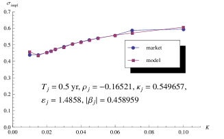
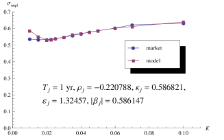
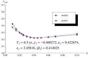
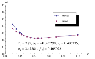
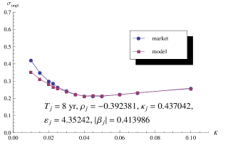
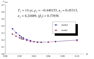
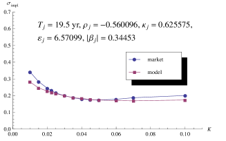
Figure 1: Implied caplet volatilities due to market data vs. calibrated model

5 Swap rate dynamics and approximate swaption pricing

5.1 Swap contracts and dynamics under swap measures

An interest rate swap is a contract to exchange a series of floating interest payments in return for a series of fixed rate payments. Consider a series of payment dates between $T_{p+1}$ and $T_{q},\,q>p.$ At each time $T_{j+1},\,j=p,\ldots,q-1,$ the fixed leg of a (standard) swap pays $\delta_{j}K,$ whereas in return the floating leg pays $\delta_{j}L_{j}(T_{j})$ with $L_{j}(T_{j})$ being the spot Libor rate. Consequently, the time $t-$value of the interest rate swap (with $t\leq T_{p}$) is

$$\sum_{j=p}^{q-1}\delta_{j}B_{j+1}(t)(L_{j}(t)-K).$$

The swap rate $S_{p,q}(t)$ is defined to be the value of $K$ for which the present value of the contract is zero. We thus have

$$S_{p,q}(t)=\frac{\sum_{j=p}^{q-1}\delta_{j}B_{j+1}(t)L_{j}(t)}{\sum_{j=p}^{q-1}\delta_{j}B_{j+1}(t)}=\frac{B_{p}(t)-B_{q}(t)}{\sum_{j=p}^{q-1}\delta_{j}B_{j+1}(t)}.$$ (34)

So $S_{p,q}$ is a martingale under the probability measure $P_{p,q}$, induced by the annuity numéraire

$$B_{p,q}(t):=\sum_{j=p}^{q-1}\delta_{j}B_{j+1}(t).$$

From (18) it follows that

$$dS_{p,q}(t)=S_{p,q}(t)\Lambda_{p,q}^{\top}(t)d\mathcal{W}^{p,q}(t),$$ (35)

where $\mathcal{W}^{(p,q)}:=(W^{p,q},\widehat{W}^{p,q})$ is standard Brownian motion under $P_{p,q},$ and where

$$\Lambda_{p,q}=\sum_{j=p}^{q-1}\frac{\delta_{j}\left(L_{j}+\alpha_{j}\right)}{1+\delta_{j}L_{j}}\left(\sum_{l=j}^{q-1}w_{l}^{p,q}+\frac{B_{q}}{B_{p}-B_{q}}\right)\left[\begin{array}[c]{c}\sqrt{v_{j}}\beta_{j}\\[8.5359pt] \gamma_{j}\end{array}\right],~{}w_{l}^{p,q}:=\frac{\delta_{l}B_{l+1}}{B_{p,q}}.$$ (36)

The derivation hereof is given in Appendix 6. We further have (see Appendix 6),

$$d\mathcal{W}^{p,q}=d\mathcal{W}^{(n)}-dt\sum_{l=p}^{q-1}w_{l}^{p,q}\sum_{k=l+1}^{n-1}\frac{\delta_{k}\left(L_{k}+\alpha_{k}\right)}{1+\delta_{k}L_{k}}\left[\begin{array}[c]{c}\sqrt{v_{k}}\beta_{k}\\[8.5359pt] \gamma_{k}\end{array}\right].\text{ }$$ (37)

By (35) we thus get

$$d\ln S_{p,q} =-\frac{1}{2}\frac{1}{S_{p,q}^{2}}d\langle S_{p,q}\rangle+\frac{dS_{p,q}}{S_{p,q}}$$ (38)

$$=-\frac{1}{2}\left|\Lambda_{p,q}\right|^{2}dt+\Lambda_{p,q}^{\top}d\mathcal{W}^{p,q},$$

where by (36) we may write

$$\Lambda_{p,q}=\sum_{j=p}^{q-1}\left[\begin{array}[c]{c}\sqrt{v_{j}}\beta_{j}\\[8.5359pt] \gamma_{j}\end{array}\right]\frac{L_{j}+\alpha_{j}}{S_{p,q}}\mathfrak{\xi}_{j}^{p,q}$$ (39)

with

$$\mathfrak{\xi}_{j}^{p,q}:=\frac{\delta_{j}}{1+\delta_{j}L_{j}}\left(\sum_{l=j}^{q-1}w_{l}^{p,q}\frac{B_{p}-B_{q}}{B_{p,q}}+\frac{B_{q}}{B_{p,q}}\right).$$

(Cf. [22], (1.35), and (1.38) so we have that $\mathfrak{\xi}_{j}^{p,q}(0)\approx w_{l}^{p,q}(0)$ with equality when the yield curve is flat; hence the $\mathfrak{\xi}_{j}^{p,q}$ are approximate weights also.)

5.2 Approximate affine swap rate dynamics

In order to approximate the swap rate process with a pure square-root volatility process we introduce the process

$$dv^{p,q}=\kappa^{p,q}(\theta^{p,q}-v^{p,q})dt+\sqrt{v^{p,q}}\left(\sigma_{p,q}^{\top}dW^{(n)}+\overline{\sigma}_{p,q}^{\top}d\overline{W}^{(n)}\right),\text{ \ \ }v^{p,q}(0)=\theta^{p,q}$$ (40)

with

$$\theta^{p,q} :=\sum_{l=p}^{q-1}w_{l}^{p,q}(0)\theta_{l}$$

$$\kappa^{p,q} :=\sum_{l=p}^{q-1}w_{l}^{p,q}(0)\kappa_{l}$$

$$\sigma_{p,q} :=\sum_{l=p}^{q-1}w_{l}^{p,q}(0)\sigma_{l}$$

$$\overline{\sigma}_{p,q} :=\sum_{l=p}^{q-1}w_{l}^{p,q}(0)\overline{\sigma}_{l}.$$ (41)

By replacing in (39) all volatility processes $v_{j}$ with the, in a sense, averaged process $v^{p,q},$ and freezing Libors we arrive at the approximation

$$\Lambda_{p,q} \approx\sum_{j=p}^{q-1}\sum_{j=p}^{q-1}\left[\begin{array}[c]{c}\sqrt{v^{p,q}}\beta_{j}\\[8.5359pt] \gamma_{j}\end{array}\right]\left[\frac{L_{j}+\alpha_{j}}{S_{p,q}}\mathfrak{\xi}_{j}^{p,q}\right](0)$$

$$=\left[\begin{array}[c]{c}\sqrt{v^{p,q}}\beta_{p,q}\\[8.5359pt] \gamma_{p,q}\end{array}\right],\text{ \ \ where}$$

$$\beta_{p,q} :=\sum_{j=p}^{q-1}\beta_{j}\left[\frac{L_{j}+\alpha_{j}}{S_{p,q}}\mathfrak{\xi}_{j}^{p,q}\right](0)\text{ \ and}$$

$$\gamma_{p,q} :=\sum_{j=p}^{q-1}\gamma_{j}\left[\frac{L_{j}+\alpha_{j}}{S_{p,q}}\mathfrak{\xi}_{j}^{p,q}\right](0)$$

(note that $\sum_{j=p}^{q-1}\mathfrak{\xi}_{j}^{p,q}\left(L_{j}+\alpha_{j}\right)/S_{p,q}\approx 1$), hence yielding affine approximative swap rate dynamics

$$d\ln S_{p,q}=-\frac{1}{2}v^{p,q}\left|\beta_{pq}\right|^{2}dt-\frac{1}{2}\left|\gamma_{p,q}\right|^{2}dt+\sqrt{v^{p,q}}\beta_{p,q}^{\top}dW^{p,q}+\gamma_{p,q}^{\top}d\widehat{W}^{p,q}.$$ (42)

For the (approximate) dynamics of $v^{p,q}$ under the annuity Brownian motions we replace in (37) the processes $v_{j}$ by their average $v^{p,q},$ and freeze the Libors as usual.  From (40) we then obtain (as in Section 4, it follows again that $\overline{W}^{(n)}=\overline{W}^{p,q}$ ),

$$dv^{p,q} \approx\kappa^{p,q}(\theta^{p,q}-v^{p,q})dt+\sqrt{v^{p,q}}\overline{\sigma}_{p,q}^{\top}d\overline{W}^{(n)}$$

$$+\sqrt{v^{p,q}}\sigma_{p,q}^{\top}\left(dW^{p,q}+\sqrt{v^{p,q}}dt\sum_{l=p}^{q-1}\sum_{k=l+1}^{n-1}\left[w_{l}^{p,q}\frac{\delta_{k}\left(L_{k}+\alpha_{k}\right)}{1+\delta_{k}L_{k}}\right](0)\,\beta_{k}\right).$$

By setting

$$\widetilde{\kappa}^{p,q} :=\kappa^{p,q}-\sum_{l=p}^{q-1}\left[w_{l}^{p,q}\sum_{k=l+1}^{n-1}\frac{\delta_{k}\left(L_{k}+\alpha_{k}\right)}{1+\delta_{k}L_{k}}\right](0)\,\sigma_{p,q}^{\top}\beta_{k}$$

$$\widetilde{\theta}^{p,q} =\frac{\kappa^{p,q}\theta^{p,q}}{\widetilde{\kappa}^{p,q}},$$

we thus have (in approximation)

$$dv^{p,q}=\widetilde{\kappa}^{p,q}(\widetilde{\theta}^{p,q}-v^{p,q})dt+\sqrt{v^{p,q}}\sigma_{p,q}^{\top}dW^{p,q}+\sqrt{v^{p,q}}\overline{\sigma}_{p,q}^{\top}d\overline{W}^{p,q}.$$ (43)

5.3 Fourier based swaption pricing

A (payer) swaption over the period $[T_{p},T_{q}]$ is the option to enter at $T_{p}$ into a swap over the period $[T_{p},T_{q}]$ with strike $K.$ It follows straightforwardly that the value at time $t=0$ is given by

$$Swpn_{p,q}(K)=B_{p,q}(0)E_{p,q}\left[\left(S_{p,q}(T_{p})-K\right)^{+}\right].$$ (44)

Thus, after determining the characteristic function for $\ln\left[S_{p,q}(T_{p})/S_{p,q}(0)\right]$ we may price the option by the Carr-Madan Fourier inversion method, just like we did for caplets in Section 4.1. Recalling the analysis from Section 4.1 it follows immediately that this characteristic function is given by

$$\varphi_{p,q}(z\,;v):=E_{p,q}\left[\left.e^{\mathfrak{i}z\ln\frac{S_{p,q}(T_{p})}{S_{p,q}(0)}}\right|v_{p,q}(0)=v\right]$$ (45)

$$\exp\left(A_{p,q}(z;T_{p})+B_{p,q}(z;T_{p})v\right)\exp\left(-\frac{1}{2}\left(\mathfrak{i}z+z^{2}\right)\int_{0}^{T_{p}}\left|\gamma_{p,q}\right|^{2}ds\right),$$

where

$$B_{p,q}(z;T_{p})=\frac{a_{p,q}+d_{p,q}}{\varepsilon_{p,q}^{2}}\frac{1-e^{d_{p,q}T_{p}}}{1-g_{p,q}e^{d_{p,q}T_{p}}}$$

and

$$A_{p,q}(z;T)=\frac{\widetilde{\kappa}^{p,q}\widetilde{\theta}^{p,q}}{\left|\sigma_{p,q}\right|^{2}+\left|\overline{\sigma}_{p,q}\right|^{2}}\left\{\left(a_{p,q}-d_{p,q}\right)T_{p}-2\ln\left[\frac{e^{-d_{p,q}T_{p}}-g_{p,q}}{1-g_{p,q}}\right]\right\}$$

with

$$a_{p,q} =\widetilde{\kappa}^{p,q}-\mathfrak{i}z\sigma_{p,q}^{\top}\beta_{p.q}$$

$$d_{p,q} =\sqrt{a_{p,q}^{2}+\left|\beta_{p,q}\right|^{2}\left(\mathfrak{i}z+z^{2}\right)\left(\left|\sigma_{p,q}\right|^{2}+\left|\overline{\sigma}_{p,q}\right|^{2}\right)}$$

$$g_{p,q} =\frac{a_{p,q}+d_{p,q}}{a_{p,q}-d_{p,q}}.$$

Based on (45) the (approximate) price of a swaption with maturity $T_{p}$ and swaption leg $[T_{p},T_{q}]$ is given by

$$Swpn_{p,q}(K)=B_{p,q}(0)E_{p,q}\left[\left(S_{p,q}(T_{p})-K\right)^{+}\right]$$

$$\approx Swpn_{p,q}^{\mathcal{B}}(K)+$$ (46)

$$\frac{B_{p,q}(0)S_{p,q}(0)}{2\pi}\int_{-\infty}^{\infty}\frac{\varphi_{p,q}^{\mathcal{B}}(z-\mathfrak{i};T_{p},\theta_{p,q})-\varphi_{p,q}(z-\mathfrak{i};T_{p},\theta_{p,q})}{z(z-\mathfrak{i})}e^{-\mathfrak{i}z\ln\frac{K}{S_{p,q}(0)}}dz$$

In (46), $\varphi_{p,q}^{\mathcal{B}}$ is the characteristic function of a corresponding Black model,

$$S_{p,q}(T_{p})=S_{p,q}(0)e^{-\frac{1}{2}\left(\sigma_{p,q}^{B}\right)^{2}T_{p}+\sigma_{p,q}^{B}\sqrt{T_{p}}\varsigma},\text{ \ \ }\varsigma\in N(0,1),$$

where $\sigma_{p,q}^{B}$ is a suitably chosen volatility, and

$$Swpn_{p,q}^{\mathcal{B}}(K)=B_{p,q}(0)E_{p,q}\left(S_{p,q}(T_{p})-K\right)^{+}=B_{p,q}(0)\mathcal{B}(S_{p,q}(0),T_{p},\sigma_{p,q}^{B},K),$$

is given by Black’s formula (cf. (31)).

5.4 Putting the swaption approximation to the test

In the same spirit as we have tested the caplet price approximation in Section 4.2 we now test the above Fourier based swaption pricing method. For each pair $(p,q),$ $1\leq p<q\leq n$ ($q\neq p+1$), we replace all volatility processes $v_{j},$ $p\leq j<q,$ with $v_{p,q}$ given by (40), (41) to obtain in fact a Wu-Zhang related swaption approximation model linked to this pair $(p,q).$ We then compare the simulated $(p,q)$-swaption price due to the “true” model (18) and the model with common stochastic volatility process (40). In turn, the latter price can be accurately approximated by (46) as shown in [24]. We base the numerical experiments on the same data set as in Section 4.2.

In detail, this means that for putting up the “true” and the approximate Libor model, the initial Libors are stripped from a given spot rate curve and their values are given in Table 1, the Gaussian $\gamma$-part is deactivated by putting $\gamma_{j}\equiv 0$ and no displacement is in force by choosing $\alpha_{j}\equiv 0$. Moreover, the parametrization of the correlation structure from Section 4.3 is given by

$$r_{ij}=\exp\big{(}-0.0553|T_{i}-T_{j}|\big{)}=e_{i}^{\top}e_{j},~{}\beta_{j}=0.15e_{j},$$

with the orthonormal vectors $e_{j}$ resulting from a Cholesky decomposition of $(r_{ij})$ and $\delta_{j}=T_{j+1}-T_{j}\equiv 1.0$ and $\theta_{j}\equiv 1$ remain valid. All other simulation parameters, in particular the $\rho_{j}$’s, $\kappa_{j}$’s and $\varepsilon_{j}$’s can be found in Table 1 and we retain the diffusion coefficients

$$\sigma_{j}=\rho_{j}\varepsilon_{j}e_{j},~{}\overline{\sigma}_{j}=\sqrt{1-\rho_{j}^{2}}\varepsilon_{j}.$$

$[T_{p},T_{q}]$	Strike	Price (SE)	Approx. price (SE)	Abs. error	Rel. error
	0.000	0.1640 (2.1e-04)	0.1637 (2.1e-04)	0.00032	0.002
	0.005	0.1302 (2.0e-04)	0.1299 (2.0e-04)	0.00032	0.002
	0.010	0.0964 (1.9e-04)	0.0961 (1.9e-04)	0.00031	0.003
[2, 10]	0.015	0.0628 (1.8e-04)	0.0625 (1.8e-04)	0.00033	0.005
	0.020	0.0317 (1.5e-04)	0.0313 (1.5e-04)	0.00037	0.011
	0.025	0.0094 (9.0e-05)	0.0092 (9.0e-04)	0.00024	0.026
	0.030	0.0011 (3.0e-05)	0.0010 (2.9e-05)	0.00003	0.030
	0.000	0.1228 (2.3e-04)	0.1223 (2.3e-04)	0.00057	0.004
	0.005	0.0981 (2.2e-04)	0.0975 (2.2e-04)	0.00055	0.005
	0.010	0.0734 (2.1e-04)	0.0728 (2.1e-04)	0.00055	0.007
[4, 10]	0.015	0.0493 (2.0e-04)	0.0488 (1.9e-04)	0.00057	0.011
	0.020	0.0281 (1.6e-04)	0.0275 (1.6e-04)	0.00060	0.021
	0.025	0.0127 (1.2e-04)	0.0122 (1.1e-04)	0.00049	0.038
	0.030	0.0042 (7.1e-05)	0.0040 (6.9e-05)	0.00026	0.060
	0.000	0.2877 (4.8e-04)	0.2866 (4.8e-04)	0.00110	0.003
	0.005	0.2288 (4.6e-04)	0.2277 (4.6e-04)	0.00107	0.004
	0.010	0.1699 (4.5e-04)	0.1689 (4.4e-04)	0.00104	0.006
[4, 20]	0.015	0.1122 (4.2e-04)	0.1112 (4.2e-04)	0.00102	0.009
	0.020	0.0609 (3.5e-04)	0.0600 (3.5e-04)	0.00091	0.015
	0.025	0.0246 (2.4e-04)	0.0241 (2.4e-04)	0.00051	0.020
	0.030	0.0068 (1.2e-04)	0.0067 (1.2e-04)	0.00011	0.016
	0.000	0.1653 (4.5e-04)	0.1638 (4.4e-04)	0.00149	0.009
	0.005	0.1311 (4.4e-04)	0.1297 (4.3e-04)	0.00146	0.011
	0.010	0.0976 (4.2e-04)	0.0961 (4.1e-04)	0.00146	0.015
[10, 20]	0.015	0.0670 (3.9e-04)	0.0655 (3.8e-04)	0.00147	0.021
	0.020	0.0423 (3.3e-04)	0.0410 (3.3e-04)	0.00137	0.032
	0.025	0.0247 (2.7e-04)	0.0236 (2.6e-04)	0.00137	0.045
	0.030	0.0134 (2.0e-04)	0.0126 (1.9e-04)	0.00081	0.060

Table 3: Simulation results for payer swaptions.

To gear towards the approximate Libor model, we perform the calculation of the weighted volatility parameters $\kappa^{p,q}$, $\theta^{p,q}$, $\sigma^{p,q}$ and $\bar{\sigma}^{p,q}$ according to (41), where the frozen weights $w^{p,q}_{l}(0)$ are given in (36), so that the averaged approximate volatility process $v^{p,q}$ from (40) can be simulated. This averaged stochastic volatility is then reinserted into the Libor dynamics (16), i.e. $v^{p,q}$ virtually replaces each expiry-wise volatility $v_{j},j=p,\ldots,q-1.$ The simulations are carried out using $30,000$ Monte Carlo paths.

We calculate “true” and approximate swaption prices for the payer swaption depicted in (44) for various strike levels and swap legs $[T_{p},T_{q}]$. The results of our numerical experiments are depicted in Table 3.

The simulation results show that for swaption pricing, the approximate Libor model under one weighted stochastic volatility $v^{p,q}$ gives a surprisingly good fit to the true model dynamics (16), (14). Depending on the swap legs, absolute price deviations are in the range of basis points (for swaption maturing in two and four years) and in the range of ten basis points (for maturity ten years). Recalling that the approximation is somewhat strong as each expiry-wise volatility process $v_{j},j=p,\ldots,q-1$ is replaced by one weighted volatility process $v^{p,q}$, the numerical results reveal however that we get reasonably well behaved approximations to the “true” model.

6 Appendix

The derivation of the swap rate volatility (36) is essentially given in [22]. But in order to match to the present notation and to make reading more convenient, we now give a short recap. Let, exclusively in this section, $\sigma_{j}$ denote the volatility of the bond $B_{j},$ let $\mu_{j}$ be the drift of $B_{j},$ and $\lambda$ be the market price of risk process with respect to the driving Brownian motion $\mathcal{W=}(W,\widehat{W},\overline{W}).$ That is, in the objective measure the zero bond dynamics are of the form

$$\frac{dB_{j}}{B_{j}}=\mu_{j}dt+\sigma_{j}^{\top}d\mathcal{W}\text{ \ \ with \ \ }\mu_{j}=\sigma_{j}^{\top}\lambda,$$

and where $\sigma_{j,k}=0$ for $m+\widehat{m}<k\leq m+\widehat{m}+\overline{m}.$ Following [22, p.17], we may write

$$dB_{p,q} =\sum_{j=p}^{q-1}\delta_{j}dB_{j+1}=\cdot\cdot\cdot dt+\sum_{j=p}^{q-1}\delta_{j}B_{j+1}\sigma_{j+1}^{\top}d\mathcal{W}$$

$$=\cdot\cdot\cdot dt+B_{p,q}\sum_{j=p}^{q-1}w_{j}^{p,q}\sigma_{j+1}^{\top}d\mathcal{W}.$$

We thus have by Itô’s formula for $p\leq r\leq q,$

$$\frac{d(B_{r}/B_{p,q})}{B_{r}/B_{p,q}} =\cdot\cdot\cdot dt+\left(\sigma_{r}^{\top}-\sum_{j=p}^{q-1}w_{j}^{p,q}\sigma_{j+1}^{\top}\right)d\mathcal{W}$$

$$=\left(\sigma_{r}^{\top}-\sum_{j=p}^{q-1}w_{j}^{p,q}\sigma_{j+1}^{\top}\right)d\mathcal{W}^{p,q}$$

as $B_{r}/B_{p,q}$ is a $P_{p,q}$-martingale. We thus obtain

$$dS_{p,q}=d\frac{B_{p}-B_{q}}{B_{p,q}}=$$

$$\left[\frac{B_{p}}{B_{p,q}}\left(\sigma_{p}^{\top}-\sum_{j=p}^{q-1}w_{j}^{p,q}\sigma_{j+1}^{\top}\right)-\frac{B_{q}}{B_{p,q}}\left(\sigma_{q}^{T}-\sum_{j=p}^{q-1}w_{j}^{p,q}\sigma_{j+1}^{\top}\right)\right]d\mathcal{W}^{p,q}$$

$$=\left[\frac{B_{p}}{B_{p,q}}\sum_{j=p}^{q-1}w_{j}^{p,q}\left(\sigma_{p}^{\top}-\sigma_{j+1}^{\top}\right)-\frac{B_{q}}{B_{p,q}}\sum_{j=p}^{q-1}w_{j}^{p,q}\left(\sigma_{q}^{\top}-\sigma_{j+1}^{\top}\right)\right]d\mathcal{W}^{p,q}$$

$$=S_{p,q}\left[\frac{B_{p}}{B_{p}-B_{q}}\sum_{j=p}^{q-1}w_{j}^{p,q}\left(\sigma_{p}^{\top}-\sigma_{j+1}^{\top}\right)-\frac{B_{q}}{B_{p}-B_{q}}\sum_{j=p}^{q-1}w_{j}^{p,q}\left(\sigma_{q}^{\top}-\sigma_{j+1}^{\top}\right)\right]d\mathcal{W}^{p,q}$$

$$=S_{p,q}\left[\sum_{j=p}^{q-1}w_{j}^{p,q}\left(\sigma_{p}^{\top}-\sigma_{j+1}^{\top}\right)+\frac{B_{q}}{B_{p}-B_{q}}\sum_{j=p}^{q-1}w_{j}^{p,q}\left(\sigma_{p}^{\top}-\sigma_{q}^{\top}\right)\right]d\mathcal{W}^{p,q}$$

$$=:S_{p,q}\Lambda_{p,q}^{\top}d\mathcal{W}^{p,q}.$$

Similar to (1.13) in [22] we get

$$\Lambda_{p,q} =\sum_{j=p}^{q-1}w_{j}^{p,q}\left(\sigma_{p}-\sigma_{j+1}\right)+\frac{B_{q}}{B_{p}-B_{q}}w_{j}^{p,q}\left(\sigma_{p}-\sigma_{q}\right)$$

$$=\sum_{j=p}^{q-1}w_{j}^{p,q}\sum_{r=p}^{j}\left(\sigma_{r}-\sigma_{r+1}\right)+\frac{B_{q}}{B_{p}-B_{q}}\sum_{r=p}^{q-1}\left(\sigma_{r}-\sigma_{r+1}\right)$$

$$=\sum_{r=p}^{q-1}\left(\sigma_{r}-\sigma_{r+1}\right)\left(\sum_{j=r}^{q-1}w_{j}^{p,q}+\frac{B_{q}}{B_{p}-B_{q}}\right)$$

$$=\sum_{r=p}^{q-1}\left[\begin{array}[c]{c}\sqrt{v_{r}}\beta_{r}\\[8.5359pt] \gamma_{r}\end{array}\right]\frac{\delta_{r}\left(L_{r}+\alpha_{r}\right)}{1+\delta_{r}L_{r}}\left(\sum_{j=r}^{q-1}w_{j}^{p,q}+\frac{B_{q}}{B_{p}-B_{q}}\right).$$

Further, by (1.27) from [22], it holds that

$$d\mathcal{W}^{(n)}=d\mathcal{W}+(\lambda-\sigma_{n})dt,\text{ \ \ and \ \ }d\mathcal{W}^{p,q}=\lambda dt-\sum_{l=p}^{q-1}w_{l}^{p,q}\sigma_{l+1}dt+d\mathcal{W}.$$

Therefore, we finally have

$$d\mathcal{W}^{p,q} =d\mathcal{W}^{(n)}+\sigma_{n}dt-\sum_{l=p}^{q-1}w_{l}^{p,q}\sigma_{l+1}dt$$

$$=d\mathcal{W}^{(n)}+dt\sum_{l=p}^{q-1}w_{l}^{p,q}\left(\sigma_{n}-\sigma_{l+1}\right)$$

$$=d\mathcal{W}^{(n)}+dt\sum_{l=p}^{q-1}w_{l}^{p,q}\sum_{k=l+1}^{n-1}\left(\sigma_{k+1}-\sigma_{k}\right)$$

$$=d\mathcal{W}^{(n)}-dt\sum_{l=p}^{q-1}w_{l}^{p,q}\sum_{k=l+1}^{n-1}\frac{\delta_{k}\left(L_{k}+\alpha_{k}\right)}{1+\delta_{k}L_{k}}\left[\begin{array}[c]{c}\sqrt{v_{k}}\beta_{k}\\[8.5359pt] \gamma_{k}\end{array}\right].$$

References

• [1] Andersen, L. and J. Andreasen (2000). Volatility skews and extensions of the LIBOR market model. Applied Mathematical Finance, 7, 1, 1-32.
• [2] Andersen, L. and R. Brotherton-Ratcliffe (2001). Extended Libor Market Models with Stochastic Volatility. Working paper, Gen Re Securities.
• [3] Belomestny, D., S. Mathew, and J. Schoenmakers (2011). Multiple stochastic volatility extension of the Libor market model and its implementation. Monte Carlo Methods Appl. (2009), 15, no. 4, 285–310.
• [4] Belomestny, D. and J.G.M. Schoenmakers (2006). A Jump-Diffusion Libor Model and its Robust Calibration, Quant. Finance, 11, pp. 529–546.
• [5] Benhamou, E., E. Gobet, and M. Miri (2010). Time dependent Heston model. SIAM Journal on Financial Mathematics, 1, pp.289-325, 2010.
• [6] Brigo, D. and F. Mercurio (2001). Interest rate models—theory and practice. Springer Finance. Springer-Verlag, Berlin.
• [7] Brace, A., Gatarek, D. and M. Musiela (1997). The Market Model of Interest Rate Dynamics. Mathematical Finance, 7 (2), 127–155.
• [8] Carr, P. and D. Madan (1999). Option Valuation Using the Fast Fourier Transform, Journal of Computational Finance, 2, 61–74.
• [9] Eberlein, E. and F. Özkan (2005). The Lévy Libor model, Finance Stoch. 7, no. 1, 1–27.
• [10] Glasserman, P. (2004). Monte Carlo methods in financial engineering. Applications of Mathematics (New York), 53. Stochastic Modelling and Applied Probability. Springer-Verlag, New York.
• [11] Glasserman, P. and S.G. Kou (2003). The term structure of simple forward rates with jump risk. Mathematical Finance, 13, no. 3, 383–410.
• [12] Hagan, P. and A. Lesniewski (2008). LIBOR market model with SABR style stochastic volatility. Working paper.
• [13] Heston, S. (1993). A closed-form solution for options with stochastic volatility with applications to bond and currency options. The Review of Financial Studies, 6, No. 2, 327-343.
• [14] Jamshidan, F.(1997). LIBOR and swap market models and measures. Finance and Stochastics, 1, 293–330.
• [15] Jamshidian, F.(2001). LIBOR Market Model with Semimartingales, in “Option Pricing, Interest Rates and Risk Management”, Cambridge Univ.
• [16] Joshi, M. and R. Rebonato (2001). A stochastic-volatility, displaced-diffusion extension of the LIBOR market model. Working paper, Royal Bank of Scotland.
• [17] Lord R. and C. Kahl (2010). Complex logarithms in Heston-like models. Math. Fin., 20, Issue 4, 671–694.
• [18] Miltersen, K., K. Sandmann, and D. Sondermann (1997). Closed-form solutions for term structure derivatives with lognormal interest rates. Journal of Finance, 409-430.
• [19] Morini, M., and F. Mercurio (2007). No-arbitrage dynamics for a tractable SABR term structure LIBOR model, preprint.
• [20] Piterbarg, V. (2004). A stochastic volatility forward Libor model with a term structure of volatility smiles. SSRN Working Paper.
• [21] Papapantoleon, A., J. Schoenmakers and D. Skovmand (2011). Efficient and accurate log-Levy approximations to Levy driven LIBOR models. J. of Computational Finance (to appear).
• [22] Schoenmakers, J. (2005). Robust Libor Modelling and Pricing of Derivative Products. Boca​​ Raton London New​​ York Singapore: Chapman & Hall – CRC Press.
• [23] Wu, L. and F. Zhang (2006). Libor Market Model with Stochastic Volatility. Journal of Industrial and Management Optimization, 2, 199–207.
• [24] Wu, L. and F. Zhang (2008). Fast swaption pricing under the market model with a square-root volatility process. Quantitative Finance, 8, (2), 163–180.