The potential approach in practice

1 Introduction.

The basics of what has become known as the potential approach to the modelling of interest rate and FX derivatives have been around for a number of years, and were presented definitively in [3]. It is well known that the time-$t$ price $Y_{t}$ of a contingent claim $Y_{T}$ to be paid at time $T>t$ can be represented as

$$Y_{t}=E[\,\zeta_{T}Y_{T}\,|\,{\cal F}_{t}\,]/\zeta_{t}$$ (1)

where $\zeta$ is the so-called state-price density process. The pricing relation (1) is the foundation of the quantitative theory of finance, and can be shown to follow very simply from axioms of linearity, positivity and time-consistency; see, for example, [4]. The state-price density is commonly interpreted as

$$\zeta_{t}=\exp\{-\int_{0}^{t}r_{s}\ ds\}Z_{t}$$ (2)

where $r$ is the riskless interest rate, and $Z$ is the likelihood-ratio martingale which transforms from the reference measure $P$ to the pricing measure $P^{*}$. For those coming from an economics training, rather than from mathematical finance, the state-price density would bear the interpretation

$$\zeta_{t}=U^{\prime}(t,c_{t})$$

as the marginal utility of optimal consumption for an agent in a general equilibrium. However one derives the state-price density, the pricing relation (1) takes the same form.

The process $\zeta$ is a positive supermartingale (if the riskless rate $r$ in (2) is non-negative), and the essential of the potential approach is to model the state-price density process directly. One way this can be done is to represent the potential as

$$\zeta_{t}=E[A_{\infty}-A_{t}\,|\,{\cal F}_{t}\,]$$ (3)

for some integrable increasing process $A$; this is in effect what Flesaker & Hughston do [2]. However, for the purposes of calibration, we need a more concrete representation, and the initial attempts at calibration always built the positive supermartingale $\zeta$ in terms of some Markov process. The seminal paper [3] studied a range of diffusion examples, which [6] fitted to interest-rate data, with modest success. Taking the underlying Markov process to be a finite-state chain seemed to fare better; see [5]. This is the approach we adopt here, with some slight variation.

To explain in more detail, we shall suppose that there is a finite-state Markov chain $X$ taking values in a finite set $I$, with intensity matrix $Q$, and we shall represent the state-price density process as

$$\zeta_{t}=f(X_{t})\exp(-\int_{0}^{t}\alpha(X_{s})\;ds)$$ (4)

for some positive functions $\alpha,f:I\rightarrow(0,\infty)$. In order that the recipe (4) defines a supermartingale, we expand using Itô’s formula to learn that we shall have to have

$$(\alpha-Q)f\equiv g\geq 0,$$ (5)

and any non-negative $g$ determines a supermartingale when we take $f=(\alpha-Q)^{-1}g$. Therefore a positive supermartingale (and so a pricing model) is specified by the triple $(Q,\alpha,g)$, where $Q$ is a Markov chain intensity matrix, and $\alpha$ and $g$ are non-negative functions.

As is explained in [3], we can take (4) and (2) to discover that

$$d\zeta_{t}\doteq-r_{t}\zeta_{t}\;dt\doteq-(\alpha-Q)f(X_{t})e^{-\int_{0}^{t}\alpha(X_{s})\;ds}\;dt$$

and hence that

$$r_{t}=\frac{g(X_{t})}{f(X_{t})}=\alpha(X_{t})-\frac{Qf(X_{t})}{f(X_{t})}.$$ (6)

Though this is quite explicit, we have little use of this expression for the spot rate, as all calculations are handled directly through the state-price density parametrized by

$$\Theta\equiv(Q,\alpha,g).$$ (7)

There are certain redundancies in this parametrization; for example, since the row sums of $Q$ must be zero, we only need to record the off-diagonal entries. Similarly, for any positive $\lambda$, the function $\lambda g$ generates the same model as the function $g$, so we may restrict attention to the reduced parameter vector

$$\theta\equiv((q_{ij})_{i\neq j},\alpha,(g_{i})_{i>1}).$$

In practice, since the entries of this vector are non-negative, we suppose they are positive and work instead with

$$\theta\equiv((\log q_{ij})_{i\neq j},\log\alpha,(\log g_{i})_{i>1}).$$ (8)

2 Calibration: particle filtering

The potential approach is envisaged as being a framework for simultaneously pricing all derivatives of interest, be they interest rate, credit, equity, FX, hybrid, $\ldots$. Of course, this is likely to be overambitious, but even if we were to regard it as only being suitable for explaining the prices of interest-rate derivatives in one currency, we have to recognise that for the pricing of a general derivative, there will be no closed-form expression, and so we will have to resort to some numerical integration. This inevitably means doing a finite sum, and so the philosophy adopted here is that we will deal only with Markov processes which take finitely many values, that is, finite-state Markov chains; thus the derivative-pricing calculation will be an exact calculation (not an approximation to an integral), and this calculation will call on nothing more sophisticated than (very fast) linear algebra operations. For example, and in particular, pricing of an American option will involve the optimal stopping of a finite-state Markov chain, which is not too difficult to do. We shall in practice rarely find any benefit in using more than 10 states for the Markov chain.

A philosophical objection to this approach is that if we work with a Markov chain with only (say) 5 states, then at any given time, the model would only allow a given derivative to have 5 possible values, which is hard to believe in the light of the fluctuating behaviour of market prices of swaptions, for example. We shall get round this objection, and address the concrete questions of calibration, by using a particle filtering point of view.

Particle filtering is a computational Bayesian methodology for filtering the state of a hidden (discrete-time) Markov process $(x_{t})$ from observations $(Y_{t})$. We suppose that the Markov process has transition density $p(x^{\prime}|x)$, and that the likelihood of the observation $y$ given the (hidden) state $x$ is $f(y|x)$. The posterior likelihood $\pi_{t}$ at time $t$, is approximated by a finite collection of point masses:

$$\pi_{t}\simeq\sum_{i=1}^{N}w_{t}^{i}\delta_{x_{t}^{i}}.$$ (9)

The updating step from one time $t$ to the next $t^{\prime}$ is achieved by moving each particle $x_{t}^{i}$ to a randomly-chosen position $x_{t^{\prime}}^{i}$ according to a density $q(\cdot|x_{t}^{i},y_{t^{\prime}})$ which may depend on the next observation. The simplest proposal density $q$ would simply be the transition density $p$, but we have to be able to tilt the proposal density towards the new data point. Having chosen the new points, we re-weight them by

$$w_{t+1}^{i}\propto\frac{w_{t}^{i}\,p(x_{t^{\prime}}^{i}|x_{t}^{i})}{q(x_{t^{\prime}}^{i}|x_{t}^{i},y_{t^{\prime}})}f(y_{t^{\prime}}|x_{t^{\prime}}^{i}),$$ (10)

where the constant of proportionality is such as to make the weights sum to one.

The particle-filtering methodology is a simple generic method, universally applicable, and as such, dependent on careful tailoring to work well on any given example; any special features must be understood and exploited if the methodology is to succeed. Here are some of the particular features of our situation.

(1) The Markovian state is $x=(\xi,\theta)$, where $\xi$ is a finite-state Markov chain. Since parameters do not change, if we just update by the transition density we will never change the set of possible values of the parameter $\theta$, so the posterior can never move to the true value. Clearly this is unsatisfactory, so we will introduce a (small) ‘shake’ of the parameters at each step, shifting $\theta$ to $\theta^{\prime}$ according to transition density $\kappa(\theta,\theta^{\prime})$. In terms of the theory, this corresponds to approximating the posterior $\pi_{t}$ not by (9) but by

$$\pi_{t}\simeq\sum_{i=1}^{N}w_{t}^{i}\;\delta_{\xi_{t}^{i}}\otimes\kappa(\theta_{t}^{i},\cdot).$$ (11)

Operationally, we are introducing a simulated annealing step, and we continue to denote by $p(\cdot|\cdot)$ the transition density of the $x_{t}$, although this now incorporates the possible movement of the $\theta$-values. We tried various forms of $\kappa$; gaussian, mutivariate-$t$, or Laplace.

However, simply shaking the parameters $\theta$ and trusting to the particle-filtering algorithm is not satisfactory in this application, since the dimension of the space is typically too large. For the success of the method, it is crucial that updates of the particles are importance-sampled as we now describe.

The new observation $y_{t}$ is a vector of asset prices which we imagine are modelled as a function $\eta(x)$ of some unknown $x=(\xi,\theta)$, plus some noise. We suppose that the likelihood of $y_{t}$ given $x$ is of the form

$$f(y|x)=\varphi_{Y}(\log y-\log\eta(x))$$

for some suitable density $\varphi_{Y}$ concentrated around zero, and initially we simply seek out the maximum-likelihood estimator of $\theta$:

$$\theta^{*}=\hbox{\rm arg max}\;f(y_{t}|(1,\theta)).$$ (12)

This step is quite computationally intensive (we use a combination of gradient search methods, and simulated annealing), but seems to be unavoidable. Notice that the $\theta^{*}$ identified does not depend in any way on the previous particle population. However, we use the MLE $\theta^{*}$ to pull the proposed values of $\theta$ into a plausible region, and then we reweight them. In more detail, for a given particle $x^{i}_{t-1}=(\xi_{t-1}^{i},\theta_{t-1}^{i})$ we first generate a new $\theta$-value $\theta_{t}^{i}$ according to a density $\varphi_{\theta}(\cdot-\theta^{*})$, and move the state $\xi$ according to the dynamics implied by the newly-chosen $\theta$-value, creating the new particle $x_{t}^{i}$. The new weight attached to this particle is proportional to

$$w_{t-1}^{i}\;\frac{p(x_{t}^{i}|x_{t-1}^{i})f(y_{t}|x_{t}^{i})}{\varphi_{\theta}(\theta^{i}_{t}-\theta^{*})}.$$

(2) The model price is the population average of the individual particle prices. This is a straightforward application of Bayesian ideas; given some derivative, and a posterior $\pi_{t}$ given in the form (9), we calculate the particle price $\eta(x_{t}^{i})$ of the derivative for each particle, and then take as the model price the average

$$\sum_{i=1}^{N}w_{t}^{i}\,\eta(x_{t}^{i}).$$

Contrast this with what would happen were we to try to follow some classical maximum-likelihood approach. At each time, we would calculate some MLE of the parameters of the problem, and then we are faced with the philosophical difficulty that if we believe that the current MLE is the truth, then the price for any given asset can only take $n$ values (where $n$ is the number of states of the chain.) The Bayesian approach glides over this problem; at any time, the price of a derivative is some posterior average of the prices which would arise under different models, and different values of the state of the chain, so there is no problem of there being conceptually only a small number of possible prices. Moreover, the Bayesian particle-filtering approach gives us at any stage a posterior distribution for the price of any derivative, and could be used provide confidence intervals for the price. This could have important practical applications; industry calibrations typically insist on exact matching of ‘the’ market prices of the calibration instruments, and this leads to some very silly modelling - in fact, fitting, not modelling. But an approach which computes confidence intervals for prices reflects uncertainty in the outputs of the model, driven by the uncertainty in the inputs to the model, and would allow a successful calibration to be defined in terms of ‘the’ calibration prices lying inside some confidence interval.

Implementing the particle filtering algorithm requires some care. There is the generic problem of impoverishment, where after a time all but a few of the particles have almost zero weight, so that evolving those particles is a waste of effort. We deal with this problem by the usual resampling technique. Next there is the problem of choosing the ‘shake’, expressed through the transition density $\kappa$. What should be the distribution of the shake, how should it be scaled? But the most important problem is finding the optimal parameters $\theta^{*}$. As a numerical method which is capable of finding a global minimum we use a combination of gradient methods to converge to local minima, and simulated annealing steps to try to avoid non-global minima. The curse of dimensionality makes it very hard to obtain nearly optimal solutions for more than 10 markov states (10 markov states then the space of parameters $\theta$ is of dimension $109$). Some ideas help to reduce the dimensionality.

Based on many simulations we find that restricting the $Q$ matrix to be a nearest-neighbour Markov chain on a circular state-space does not necessarily reduce the quality of fit. In fact, MLEs obtained by simulated annealing with a full $Q$ matrix and nearest-neighbour chain give fits of similar quality. The dimensionality reduction in $\theta=(Q,\alpha,g)$ obviously helps the numerical optimisation algorithm. However, if $Q$ was restricted to a nearest-neighbour Markov chain on a circle that was only allowed to travel in one direction, then the quality of fit is much worse.

3 The data.

The data we worked with was daily data for the period 23rd April 2003 until 1st January 2007, and consisted of

• LIBOR rates: 1m, 3m, 6m, 12m

• Swap rates: 2y, 3y, 5y, 7y, 10y

• Cap prices: 1y, 3y, 5y, 7y, 10y (at-the-money strike)

• Swaption prices: 6m, 1y, 2y, 3y, 5y into 2y, 3y, 5y, 7y, 10y (at-the-money strike)

in four currencies (USD, EUR, GBP, JPY), along with FX forwards into USD of the other three currencies, looking ahead 1m, 3m, 6m, 1y. For swap, swaptions and caps, payments are quarterly. The data were quite clean, and represented an excellent source to work from.

4 Results of the fitting.

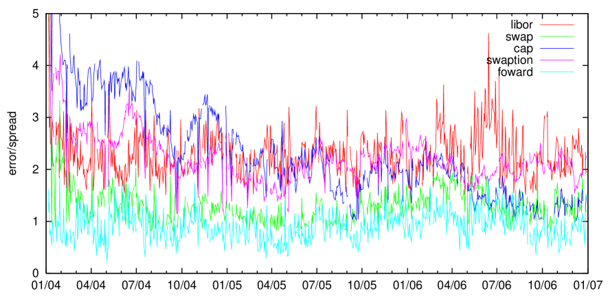
Figure 2: Average absolute errors in spreads.

We present various plots to summarise the quality of the fits. In the first, Figure 2, we show how the average absolute errors (measured in spreads) vary across time. The averages are split according to the types of instrument. It is interesting to note that for FX forwards and swaps the average error is typically no bigger than 1.5 spreads, and for caps, swaptions, and Libor rates the errors are of the typical order of 2.5 spreads.

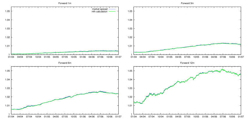
Figure 3: Forward JPY rates.

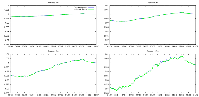
Figure 4: Forward GBP rates.

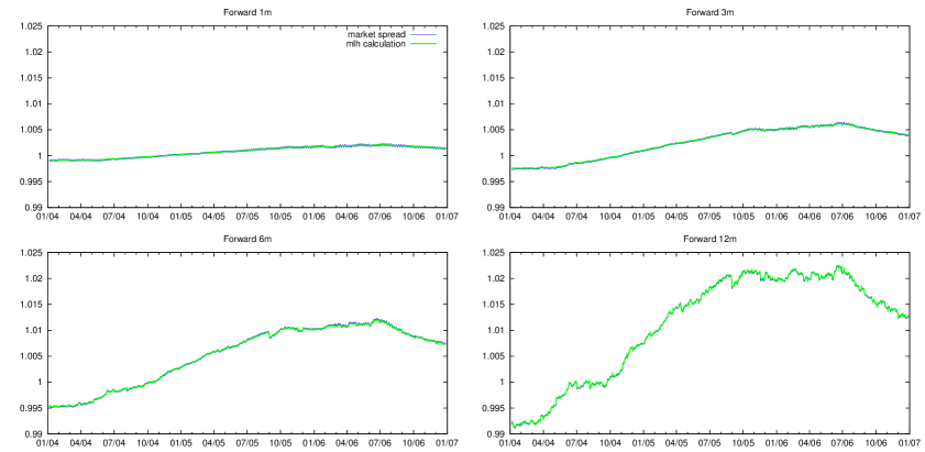
Figure 5: Forward EUR rates.

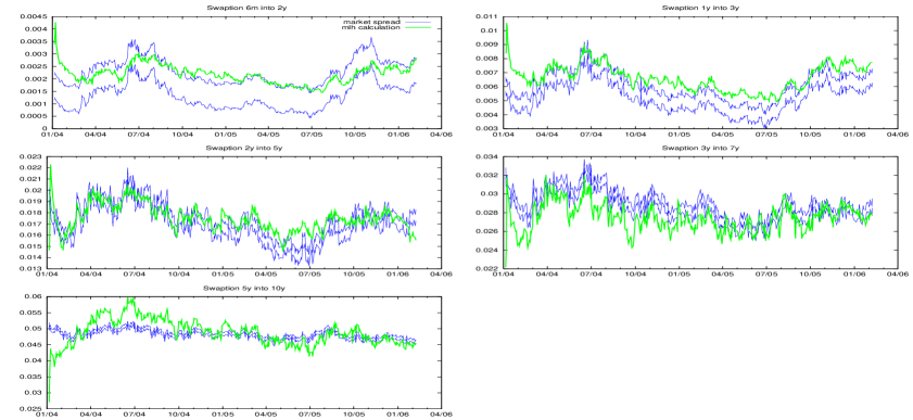
Figure 6: JPY swaption prices.

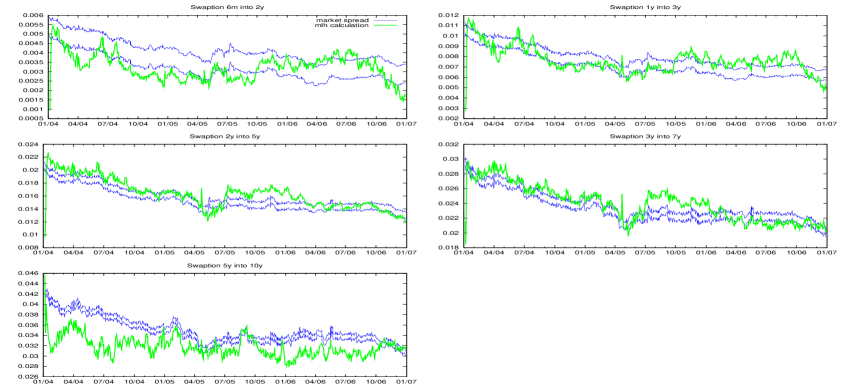
Figure 7: GBP swaption prices.

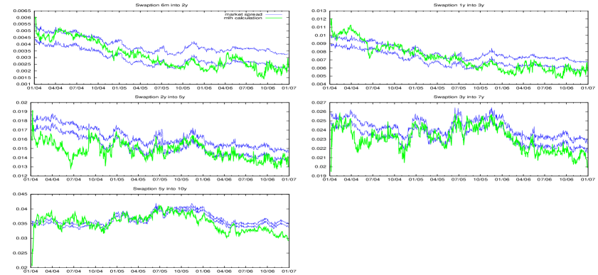
Figure 8: EUR swaption prices.

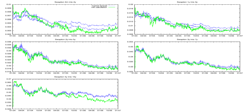
Figure 9: USD swaption prices.

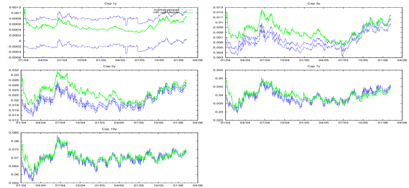
Figure 10: JPY cap prices.

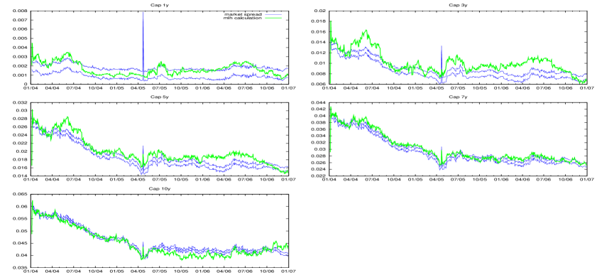
Figure 11: GBP cap prices.

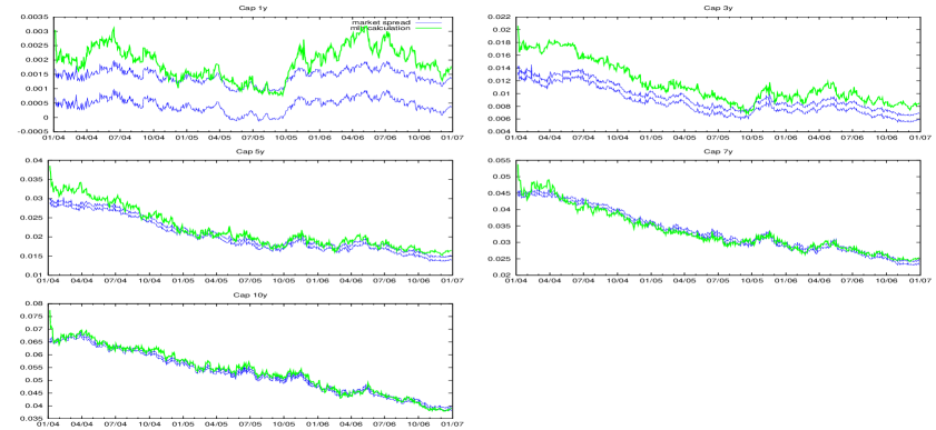
Figure 12: EUR cap prices.

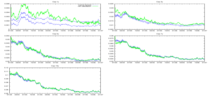
Figure 13: USD cap prices.

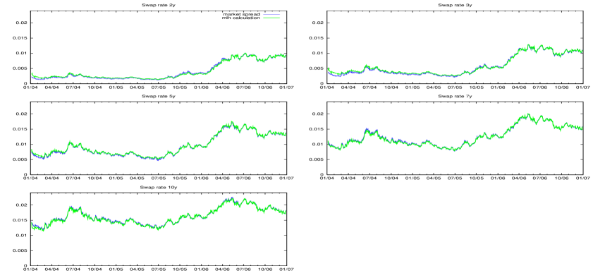
Figure 14: JPY swap rates.

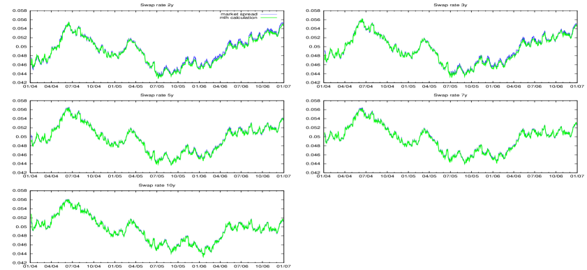
Figure 15: GBP swap rates.

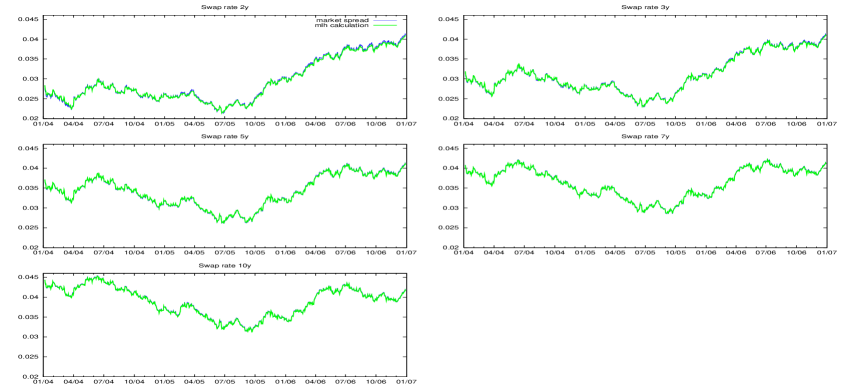
Figure 16: EUR swap rates.

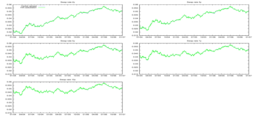
Figure 17: USD swap rates.

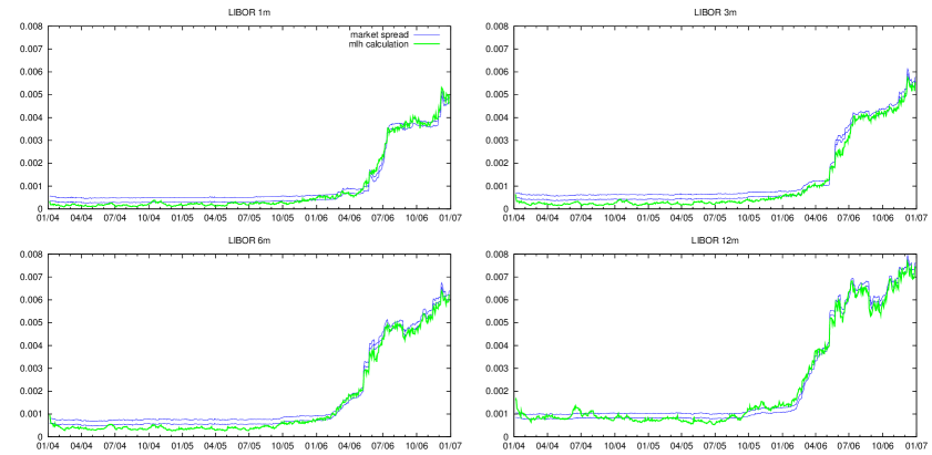
Figure 18: JPY Libor rates.

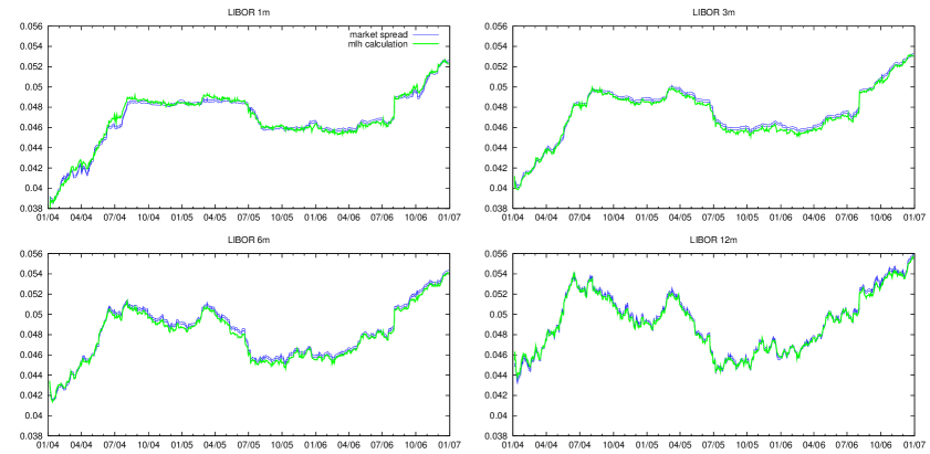
Figure 19: GBP Libor rates.

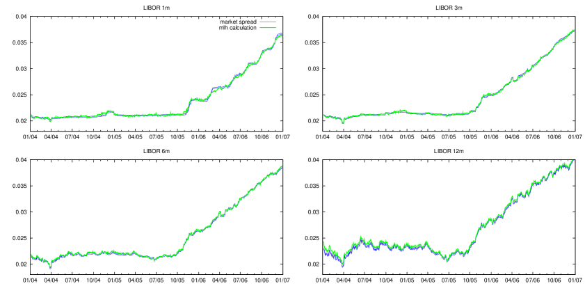
Figure 20: EUR Libor rates.

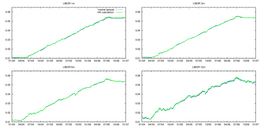
Figure 21: USD Libor rates.

There follow a number of plots of the ML fitted values (in green) and the corresponding market bids and asks (in blue) for various series: FX forward rates (Figures 3, 4, 5); swaption prices (Figures 6, 7, 8, 9); cap prices (Figures 10, 11, 12, 13); swap rates (Figures 14, 15, 16, 17); Libor rates (Figures 18, 19, 20, 21). The quality of the fits is visible from these plots. Perhaps the caps work least well, with the swaptions also less good than the FX forwards, the swap reated and the Libor rates. It is perhaps not too surprising that the OTC derivatives are less well fitted than the more liquid fundamentals, but this does highlight an area for further work. For example, we have only reported on the fits obtained with nearest-neighbour Markov chains on a circular state-space, and with never more than 7 states. There is therefore scope to improve the fit by relaxing these restrictions, but the increased dimensionality that would follow may mean that the fit is not much improved, if at all. We hope to be able to follow this further in subsequent work.

5 Hedging.

In conventional models, the standard way to hedge a derivative is to delta-hedge it. We compute the differential of the price of the derivative with respect to the prices of the underlying instruments, and this tells us how many units of the underlying to hold to protect (to leading order) against the moves in the underlying. In the case of a complete market, this hedging methodology perfectly replicates the contingent claim we were trying to hedge.

If we are using a Markov chain potential model, the notion of differentiating has no meaning, nevertheless the idea of immunising our portfolio against possible changes will work just as well. Suppose that we have a derivative $Z$, and hedging instruments $z^{(1)},z^{(2)},\ldots$. Suppose that if the state of the chain at time $t$ is $i$ and it jumps to $j$ then the value of $Z$ changes by $\Delta Z_{ij}(t)$. Then what we will do is to hold $w_{r}(t)$ units of asset $r$ so that

$$\Delta Z_{ij}(t)+\sum_{r=1}^{m}\;w_{r}(t)\Delta z^{(r)}_{ij}(t)=0\quad\forall j\quad(X_{t}=i).$$ (13)

Thus whatever jumps of the chain occur, our hedging portfolio will be unaffected by them. Of course, we do not in practice know $X_{t}$, but this does not alter the hedging methodology; we would now make a portfolio of more hedging assets so as to ensure that

$$\Delta Z_{ij}(t)+\sum_{r=1}^{M}\;w_{r}(t)\Delta z^{(r)}_{ij}(t)=0\quad\forall i,j.$$ (14)

Following this recipe in the case of (say) a 5-state chain would entail taking a position in 20 different hedging instruments (if that many were available!)

In the context of the particle-filtering modelling, the simplest thing we could propose is to calculate the hedging requirement for each particle in the population using the analysis of (13) above (recall that each particle thinks it knows for certain what the state of the chain is). Taking a weighted average of the individual particles’ hedging requirements then gives a first candidate for the hedge.

In Figure 1 we see how this simple-minded procedure performed when we tried to hedge a 5-into-2 year swaption using some caps The hedge is fitting the market price generally as well as the model, and also appears to be tracking the underlying very well; rises and falls in the underlying are accompanied by corresponding rises and falls in the value of the hedge.

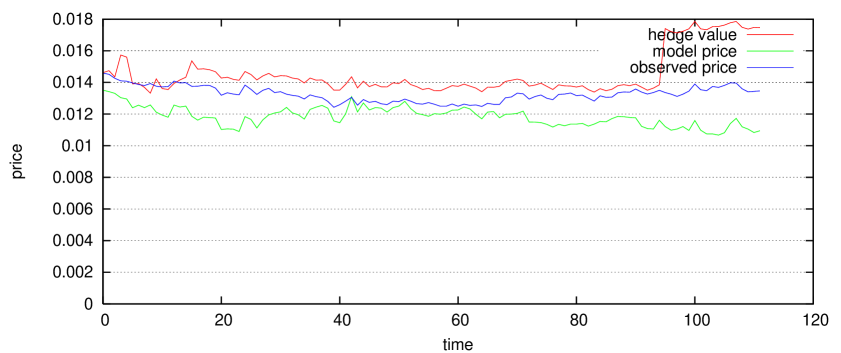
Figure 1: Here we hedge a swaption 5 into 2 years by caps: 1, 3, 5, 7, 10 years in a 5 state chain.

6 Conclusions.

The calibration study conducted in this paper is a major and ambitious test of the concept that the potential approach may account simultaneously for the prices of many assets in different currencies. Altogether, across the four currencies considered, we were computing simultaneously the prices of 168 instruments, and after time for the particle-filtering algorithm to bed in, we were able to fit market prices to within an average error of a few spreads for all the instruments, sometimes much better. The simple-minded hedging rules suggested by the modelling approach gave hedge values which were quite close to the underlying, and tracked well in the sense that the increments processes looked quite similar.

There remain further challenges to tackle, particularly in extending the calibration to other classes of assets. The extension to credit derivatives is mathematically relatively straightforward; the default of a firm is modelled by a credit spread which depends on the state of the Markov chain $\xi$, and this then needs to be estimated. What is easy about this is that the pricing of CDOs and CDS is mathematically very similar to pricing of riskless interest-rate derivatives. What is less appealing is the feature that one may need in principle a different credit spread function for each firm, hugely increasing the dimension of the problem. We expect that the correct approach to this is to firstly fit and fix the model for riskless interest rates, and then calibrate firm- or sector-specific default intensities thereafter.

The next more challenging issue is to try to fit equities to the modelling framework. At one level, this need not be so hard, if we model the price of a stock as the NPV of all future dividends, and then try to write the dividend process as a function of the underlying Markov chain $\xi$. This introduces (in principle) a separate function for each stock being considered, and again the approach will be to fit the model to the big fixed-income, futures, FX data, then try to fit the individual stock characterstics into that model. However, it may turn out to be necessary to introduce individual Brownian terms into the individual stock. At very least, some translation of the proposed (discrete state space) model into the more familiar terms of growth rate and volatility will be necessary.

These are issues which remain to be tackled, and we hope that these will be dealt with shortly. However, what is clear is that the Markov chain potential approach which we advocate in the study has shown an amazing capacity provide a model which closely fits major fixed-income and FX assets in multiple currencies. This is important at various levels, not least that it offers a framework for the pricing and hedging of hybrid derivatives of arbitrary complexity. The fitted model is not merely a fit; it makes predictions about the co-movement of many assets, and so could for example be used to price quite complicated credit derivatives (a theme developed in the study [1]).

References

- [1] G. Di Graziano and L. C. G. Rogers. A dynamic approach to the modelling of correlation credit derivatives using markov chains. Technical report, University of Cambridge, 2005.
- [2] B. Flesaker and L. P. Hughston. Positive interest. RISK, 9:46–49, 1996.
- [3] L. C. G. Rogers. The potential approach to the term structure of interest rates and foreign exchange rates. Mathematical Finance, 7:157–176, 1997.
- [4] L. C. G. Rogers. The origins of risk-neutral pricing and the Black-Scholes formula. In C. O. Alexander, editor, Handbook of Risk Management and Analysis, pages 81–94. Wiley, Chichester, 1998.
- [5] L. C. G. Rogers and F. A. Yousaf. Markov chains and the potential approach to modelling interest rates and exchange rates. In S. R. Pliska & T. Vorst H. Geman, D. Madan, editor, Mathematical Finance - Bachelier Congress 2000, pages 375–406. Springer, Berlin, 2002.
- [6] L. C. G. Rogers and O. Zane. Fitting potential models to interest rates and foreign exchange rates. In L. P. Hughston, editor, Vasicek and beyond, pages 327–342. RISK Publications, London, 1997.