Numerical Simulation of Solar Microflares in a Canopy-Type Magnetic Configuration

Abstract

Microflares are small activities in solar low atmosphere, some are in the low corona, and others in the chromosphere. Observations show that some of the microflares are triggered by magnetic reconnection between emerging flux and a pre-existing background magnetic field. We perform 2.5D compressible resistive MHD simulations of magnetic reconnection with gravity considered. The background magnetic field is a canopy-type configuration which is rooted at the boundary of the solar supergranule. By changing the bottom boundary conditions in the simulation, new magnetic flux emerges up at the center of the supergranule and reconnects with the canopy-type magnetic field. We successfully simulate the coronal and chromospheric microflares, whose current sheets are located at the corona and the chromosphere, respectively. The microflare of coronal origin has a bigger size and a higher temperature enhancement than that of chromospheric origin. In the microflares of coronal origin, we also found a hot jet ($\sim$$1.8\times 10^{6}$ K), which is probably related to the observational EUV/SXR jets, and a cold jet ($\sim$$10^{4}$ K), which is similar to the observational H$\alpha$/Ca surges, whereas there is only an H$\alpha$/Ca bright point in the microflares of chromospheric origin. The study of parameter dependence shows that the size and strength of the emerging magnetic flux are the key parameters which determine the height of the reconnection location, and further determine the different observational features of the microflares.

1 INTRODUCTION

Microflares, or subflares, which are small-scale and short-lived solar activities, have already been studied for many years since last century  (Smith & Smith, 1963; Svestka, 1976; Tandberg-Hanssen & Emslie, 1988). The typical size, duration and total released energy are 5–20 arcsecs, 10–30 minutes and $10^{26}$–$10^{29}$ ergs (Shimizu et al., 2002; Fang et al., 2006, 2010), respectively. Microflares have been observed in many wavelengthes including H$\alpha$ (Schmieder et al., 1997; Chae et al., 1999; Tang et al., 2000), EUV (Emslie & Noyes, 1978; Porter et al., 1984; Chae et al., 1999; Brosius & Holman, 2009; Chen & Ding, 2010), soft X-ray (Golub et al., 1974, 1977; Tang et al., 2000; Shimizu et al., 2002; Kano et al., 2010), hard X-ray (Lin et al., 1984; Qiu et al., 2004; Ning, 2008; Brosius & Holman, 2009), and microwave (Gary & Zirin, 1988; Gopalswamy et al., 1994; Gary et al., 1997). However, not all microflares have emissions at all wavelengths. Observations show that most of bright X-ray microflares also appear at EUV and H$\alpha$ bands, but only part of H$\alpha$ microflares have their counterparts in X-ray emission (Zhang et al., 2012).

Observational characteristics of microflares, such as the heating, the relation with magnetic field, the duration and the coincidence between different wavelengths, etc, imply that microflares are produced by magnetic reconnection, similar to big flares. For example, Qiu et al. (2004) found that about 40% of microflares show hard X-ray emissions at over 10 keV and microwave emissions at about 10 GHz, typical features for flares. Recently, Ning (2008) found that roughly half of the microflares display the Neupert effect as previously revealed in flares. On the other hand, some other microflares may have their origins in the lower atmosphere. Brosius & Holman (2009) found that the microflares are bright in the chromospheric and transition region spectral lines, which is consistent with the chromospheric heating by nonthermal electron beams. Jess et al. (2010) concluded that the microflares in their study are due to magnetic reconnection at a height of 200 km above the solar surface.

Since a part of the microflares are located at emerging flux regions, they are probably due to magnetic reconnection driven by the new emerging magnetic flux (EMF) with a pre-existing magnetic field. Schmieder et al. (1997) found that the X-ray loops of microflares appear at the locations of EMF. Chae et al. (1999) found some repeatedly occurred EUV jets where the pre-existing magnetic field was “canceled” by the new EMF with opposite polarity. Tang et al. (2000) indicated that the new EMF successfully emerged about 20 minutes before the peaks of H$\alpha$ and soft X-ray brightenings. Half of the events studied by Shimizu et al. (2002) show the small scale emergences of magnetic flux loops in the vicinity of the transient brightenings. Kano et al. (2010) found that EMFs and moving magnetic features (MMFs) are related to the energy release for at least half of the microflares around a well developed sunspot. Therefore, to understand the dynamics of microflares, it is crucial to simulate the magnetic reconnection associated with EMF.

The numerical simulations of flux emergence scenario started from 1980s (Horiuchi et al., 1988; Matsumoto et al., 1988; Shibata et al., 1989a, b). Later, more realistic and complicated numerical experiments (Magara, 2001; Fan, 2001; Manchester et al., 2004; Isobe et al., 2005; Leake & Arber, 2006; Isobe et al., 2007; Hood et al., 2009) were presented to study the emergence of twisted flux from the convection region to solar corona. The simulations are mainly based on the Parker instability which is proposed by Parker (1966) and their results can be applied to account for the formation of filament or newly active region. More 2D and 3D numerical experiments are focused on the interaction between the emerging flux and the per-existing coronal magnetic configuration to study the solar eruptions. With 2D simulations, it is found that the magnetic reconnection due to flux emergence can well explain solar jets or explosive events (Yokoyama & Shibata, 1995; Jin et al., 1996; Nishizuka et al., 2008; Ding et al., 2010, 2011), or can even trigger the onset of coronal mass ejections (Chen & Shibata, 2000). Further 3D simulations gave the same but more detailed results, which revealed that the emerging flux plays a key role in the formation of many solar activities, such as type II spicules, erupting filaments or flux ropes, Ellerman bombs, and so on (Galsgaard et al., 2005, 2007; Török et al., 2009; Archontis Török, 2008; Archontis & Hood, 2009; Martínez-Sykora et al., 2011).

From the description of previous works, it is seen that EMF is responsible for many different phenomena, and one main cause of the diversity of the dynamics is that the reconnection happens at diffferent heights in the solar atmosphere (Shibata, 1996; Chen et al., 1999). Our simulation in this paper is mainly focused on the microflares in a canopy-type magnetic configuration, where the height of the reconnection is self-consistently determined by the EMF. In our previous papers (Jiang et al., 2010; Xu et al., 2011), we presented the 2.5 dimensional (2.5D) magnetohydrodynamic (MHD) simulation of magnetic reconnection in the chromosphere, which reproduces qualitatively the temperature enhancement observed in chromospheric microflares. However, the magnetic configuration in that simulation, the same as in Chen et al. (2001), is too idealized and the reconnection site was specified at the computational center. Besides, no corona was included, so that the simulations can tell nothing about the EUV and SXR features. In this paper, we adopt a more realistic magnetic configuration and extend the solar atmosphere up to the corona in order to see what determines a microflare to be of coronal origin or of the chromospheric origin, and to compare the difference between the two types of microflares. The paper is organized as follows: the numerical method is described in Section 2; the numerical results are presented in Section 3. Discussion and summary are given in Section 4.

2 NUMBERICAL METHOD

2.1 Basic Equations

How to keep the magnetic field divergence free is one of the big problems in all MHD codes. Because of the discretization and numerical errors, the performance of the MHD code can be unphysical (Brackbill & Barnes, 1980). There are several ways to maintain $\nabla\cdot\mathbf{B}=0$ for MHD equations: (1) 8-wave formulation (Powell et al., 1999), (2) the CT method (Evans & Hawley, 1988; Stone & Norman, 1992), (3) the projection scheme (Brackbill & Barnes, 1980). The comparison between these methods showed that different methods have their own advantages and disadvantages (Tóth, 2000). Besides, one can rewrite the original MHD equations by using vector potential $\mathbf{A}$ instead of the magnetic field $\mathbf{B}$, or by using the vector magnetic potential or Euler potential. The advantage is that the divergence free condition is always satisfied, however, the MHD equation should be rewritten. Our method, as introduced in Jiang et al. (2012) adopts the 8-wave method. As suggested by Dedner et al. (2002), we use the Extended Generalized Lagrange Multiplier (EGLM)-MHD equations rather than pure MHD equations, which include two additional waves to transfer the numerical error of $\nabla\cdot\mathbf{B}$. The local divergence error can be damped and passed out of the computational domain. The adopted dimensionless EGLM-MHD equations with resistivity and gravity included are given as follows:

$$\frac{\partial\rho}{\partial t}+\nabla\cdot\left(\rho\mathbf{v}\right)=0\,\,,$$ (1)

$$\frac{\partial\left(\rho\mathbf{v}\right)}{\partial t}+\nabla\cdot\left(\left(p+\frac{1}{2}{B}^{2}\right)\mathbf{I}+\rho\mathbf{v}\mathbf{v}-\mathbf{B}\mathbf{B}\right)=-\left(\nabla\cdot\mathbf{B}\right)\mathbf{B}+\rho\mathbf{g}\,\,,$$ (2)

$$\frac{\partial\mathbf{B}}{\partial t}+\nabla\cdot\left(\mathbf{v}\mathbf{B}-\mathbf{B}\mathbf{v}+\psi\mathbf{I}\right)=-\nabla\times\left(\eta\nabla\times\mathbf{B}\right)\,\,,$$ (3)

$$\frac{\partial e}{\partial t}+\nabla\cdot\left(\mathbf{v}\left(e+\frac{1}{2}{B}^{2}+p\right)-\mathbf{B}\left(\mathbf{B}\cdot\mathbf{v}\right)\right)=-\mathbf{B}\cdot\left(\nabla\psi\right)-\nabla\cdot\left(\left(\eta\nabla\times\mathbf{B}\right)\times\mathbf{B}\right)+\rho\mathbf{g}\cdot\mathbf{v}\,\,,$$ (4)

$$\frac{\partial\psi}{\partial t}+c_{h}^{2}\nabla\cdot\mathbf{B}=-\frac{c_{h}^{2}}{c_{p}^{2}}\psi\,\,,$$ (5)

where eight independent conserved variables are the density ($\rho$), momentum ($\rho v_{x}$, $\rho v_{y}$, $\rho v_{z}$), magnetic field ($B_{x}$, $B_{y}$, $B_{z}$), and total energy density ($e$). The expression of the total energy density is $e=p/(\gamma-1)+\rho v^{2}/2+B^{2}/2$ where $\gamma=1.1$ is taken in all our computations. The pressure $p$ and temperature $T$ are dependent on the eight conserved variables, $\mathbf{g}$ is the gravity vector, and $\eta$ the magnetic resistivity coefficient. Finally, a unity matrix $\mathbf{I}$ is the unity matrix. The main variables are normalized by the quantities given in Table 1.

Table 1: Normalization Units

Variable	Quantity	Unit	Value
$T$	Temperature	$T_{0}$	$10000$ K
$\rho$	Density	$\rho_{0}$	$2.56\times 10^{-8}$ kg m-3
$x,y$	Length	$L_{0}=T_{0}\kappa_{B}/(mg_{s})$	$301.6$ km
$p$	Pressure	$p_{0}=\rho_{0}T_{0}\kappa_{B}/m$	$2.12$ N m-2
$\mathbf{V}$	Velocity	$v_{0}=(p_{0}/\rho_{0})^{1/2}$	$9.09$ km s-1
$\mathbf{B}$	Magnetic field	$B_{0}=(\mu_{0}p_{0})^{1/2}$	$16.3$ G
$t$	Time	$t_{0}=L_{0}/v_{0}$	$33.1$ s

In the EGLM-MHD equations, $\psi$ is a scalar potential propagating the divergence error, $c_{h}$ is the wave speed, and $c_{p}$ the damping rate of the wave (Dedner et al., 2002; Matsumoto, 2007). As suggested by Dedner et al. (2002), the expressions for $c_{h}$ and $c_{p}$ are:

$$c_{h}=\frac{c_{cfl}}{\Delta t}\min(\Delta x,\Delta y)\,\,,$$ (6)

$$c_{p}=\sqrt{-\Delta t\frac{c_{h}^{2}}{\ln{c_{d}}}}\,\,,$$ (7)

where $\Delta t$ is the time step, $\Delta x$ and $\Delta y$ are the grid sizes, $c_{cfl}$ is a safety coefficient less than 1. $c_{d}\in(0,1)$ is a problem dependent coefficient to decide the damping rate for the waves of divergence errors. We can see that $c_{h}$ and $c_{p}$ are not independent of the grid resolution and the scheme used. Hence we have to adjust their values for different situations.

2.2 Initial Condition

The computational box is located in the $x$-$y$ Cartesian plane. The $x$-axis is parallel to the solar surface while the $y$-axis is perpendicular to the photosphere. As shown in Figure 1, the computational domain is $-100\leq x\leq 100$ and $0\leq y\leq 200$, where the length unit is $L_{0}=301.6$ km. In the simplified chromosphere and photosphere the temperature is set uniform with the value of 0.6, after being normalized by $T_{0}=10000$ K. This layer extends from the bottom to $y=8.5$. After a thin transition region with a thickness of 1, the plasma temperature rises rapidly to 100 in the corona, which corresponds to 1 MK. Given the temperature distribution we can get the density and pressure distributions according to the hydrostatic equilibrium. The initial distributions of density, gas pressure, plasma $\beta$ (the ratio of gas to magnetic pressures) and temperature along the red line in Figure 1 are outlined by Figure 2.

As shown in Figure 1, two canopy-shaped magnetic structures are separated by a distance of 100 (corresponding to 30 Mm) in order to mimic the two boundaries of a supergranular cell. The canopy magnetic field, which was originally proposed by Gabriel (1976) and Giovanelli (1980, 1982) for studying the chromospheric and photospheric magnetic fields, is rooted at the supergranular boundaries. In order to create a canopy magnetic field, we introduce several “magnetic charges” locating beneath the photosphere. Accroding to the Gauss’s theorem in the magnetism, the magnetic field (at the position $\mathbf{r}$) generated by a “magnetic charges” (at the position $\mathbf{r^{\prime}}$) can be written as $\mathbf{B}=c_{B}(\mathbf{r}-\mathbf{r^{\prime}})/|\mathbf{r}-\mathbf{r^{\prime}}|^{2}$ in two dimensional geometry ($c_{B}$ is a constant related the strength of the field) and $\mathbf{B}=c_{B}(\mathbf{r}-\mathbf{r^{\prime}})/|\mathbf{r}-\mathbf{r^{\prime}}|^{3}$ in three dimensional geometry, which is similar to the electric field. The locations of the “magnetic charges” are depicted in Figure 1. The magnetic configuration in our simulation is not exactly the same as the canopy model proposed by Gabriel (1976) and Giovanelli (1980, 1982).

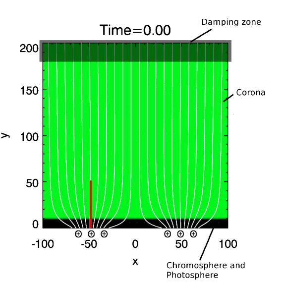
Figure 1: Initial condition for the magnetic configuration and temperature distribution. The ranges of the computational box is from $-100$ to $100$ in the $x$-direction and from $0$ to $200$ in the $y$-direction. The shadowy region means the damping zone. The “magnetic charges” are located beneath the solar surface. Note that the “magnetic charges” are samples to show the positions of these “charges”. The units of length, temperature, time and velocity are $301.6$ km, $10000$ K, $33.1$ s and $9.09$ km s^-1, respectively.

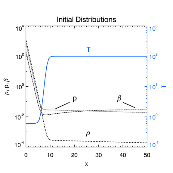
Figure 2: Initial distributions of the density ($\rho$), gas pressure ($p$), plasma beta ($\beta$) and temperature ($T$). The density, gas pressure and plasma $\beta$ distributions use the same left $y$-axis and the right blue $y$-axis is for the temperature. The units of density, gas pressure, length, temperature, time and velocity are $2.56\times 10^{-8}$ kg m^-3, $2.12$ N m^-2, $301.6$ km, $10000$ K, $33.1$ s and $9.09$ km s^-1, respectively.

2.3 Resistivity Model

In order to reproduce a fast reconnection (Petschek, 1964), we adopt a non-uniform anomalous resistivity. This kind of resistivity may be due to some microscopic instabilities, although how these instabilities drive the macroscopic reconnection is still not clear. The mathematical form of the assumed anomalous resistivity model (Ugai, 1985; Chen & Shibata, 2000; Yokoyama & Shibata, 2001) is:

$$\eta=\min\left(\left(\frac{|\mathbf{j}|}{j_{c}}-1\right),\eta_{max}\right)\ for\ |j|\geq j_{c}\,\,,$$ (8)

where $|\mathbf{j}|$ is the total current density, $j_{c}$ the threshold, above which the anomalous resistivity is excited, and $\eta_{max}$ the maximum value of the resistivity. As shown by Equations (8), the resistivity ($\eta$) is dependent on the current density. The anomalous resistivity ($\eta$) is switched off when $|\mathbf{j}|<j_{c}$.

2.4 Boundary condition

The magnetic flux emergence is realized by changing conditions at the lower boundary (Forbes & Priest, 1984; Chen & Shibata, 2000; Ding et al., 2010). In our case, $B_{x}$ and $B_{y}$, rather than the magnetic flux function in previous works, are independent variables, we change directly the magnetic field value at the boundary. The magnetic field ($B_{x}$, $B_{y}$, $B_{z}$) changes with time while the other variables, e.g., $\rho$, $\mathbf{v}$, and $p$, are fixed to the initial values at this boundary. The mathematic form of the EMF is given by:

$$B_{x}(x,y)=-B_{e}\frac{t}{t_{e}}\frac{y-y_{e}}{x^{2}+y^{2}}\,\,,$$ (9)

$$B_{y}(x,y)=B_{e}\frac{t}{t_{e}}\frac{x-x_{e}}{x^{2}+y^{2}}\,\,,$$ (10)

in the range $x^{2}+y^{2}\leq r_{0}^{2}$, $y\leq 0$, where $B_{e}$ is the strength of the EMF, $t_{e}$ the end time of emergence, $r_{0}$ the half width of the EMF, $x_{e}$ and $y_{e}$ the center coordinates of the EMF in $x$- and $y$-direction. In our simulation cases, $x_{e}$ and $y_{e}$ are set to be $0$ and $-3.6$, respectively. Formulae (9)–(10) are applied to the magnetic field $\mathbf{B}$ until $t=t_{e}$. Later, all the physical values are fixed.

Free boundaries (equivalent extrapolation) are adopted at the upper side $y=200$. However, because of the low plasma beta ($\beta=2p/\mathbf{B}^{2}$) the upper boundary becomes unstable when the jets or waves propagate to this boundary. Thus we add a damping zone from $y=180$ to $y=200$ in $y$-direction as shown in Figure 1. The waves or jets will be damped to the initial value as the formulae given below:

$$u(x,y)=u(x,y)D(y)+u_{0}(x,y)\left(1-D(y)\right)\,\,,$$ (11)

$$D(y)=\frac{1}{2}\left(1-\tanh\left(\frac{6}{y_{e}-y_{s}}\left(y-\frac{y_{s}+y_{e}}{2}\right)\right)\right)\,\,,$$ (12)

where $u$ represents varibles $\rho$, $\mathbf{v}$, and $p$ (not $\mathbf{B}$), $u_{0}$ is the initial value, $D$ the damping function, $y_{s}$ the start of position for the damping zone in $y$ direction, $y_{e}$ the end position for damping zone. In all our cases, $y_{s}=180$ and $y_{e}=200$. Nonetheless, the damping zone may also lead to some reflections of waves or jets, but these reflections have little effect on the results since they are far away from the lower atmosphere which we are interested in. We use fixed boundary condition for the left and right boundaries at $x=-100$ and $x=100$.

2.5 Numerical Scheme and AMR Grid

The code used in our simulation is MAP (Jiang et al., 2012), which is developed by the solar group of Nanjing University. The MAP code is a FORTRAN code for MHD calculation with the adaptive mesh refinement (AMR) (Berger & Oliger, 1984; Berger & Colella, 1989) and Message Passing Interface (MPI) parallelization. MAP have three optional numerical schemes for the MHD part, namely, modified Mac Cormack Scheme (Yu & Liu, 2001), Lax-Fridrichs scheme (Toth & Odstrčil, 1996) and weighted essentially non-oscillatory (WENO) (Jiang & Wu, 1999) scheme. In this paper, we mainly use the WENO scheme, which has a higher accuracy than the other two. Moreover, it can keep the total variation diminishing (TVD) (Harten, 1997) property for the MHD part without any additional artificial viscosity. The base resolution of our simulation is $256\times 256$ and the mesh refinement level is $4$ in all of our cases. Thus the effective resolution is $2048\times 2048$ globally and the minimum grid size is $0.1$ (about $30$ km).

3 RESULTS

Our simulations show two typical cases, one with the reconnection occurring in the corona while the other mainly in the chromosphere and partly in transition region. The dynamics of magnetic reconnection processes is similar in the early stage in the two cases. Both show the following evolution: (1) an EMF emerges from the center of the supergranule; (2) the EMF reconnects with the pre-existed magnetic field; (3) temperature is enhanced near the X-point and the reconnection inflow and outflow appear. However, the final results are very different. The difference between these two cases are presented in 3.1 and 3.2 subsections.

3.1 Coronal Microflare

In this case, we set the parameters of the EMF to be $B_{e}=32$ (corresponding to $520$ G), $\eta_{max}=0.1$ and $r_{0}=8$ (corresponding to $\sim 2400$ km). The reconnection occurs when the local current density is larger than the threshold ($j_{c}=10$) in the formula (8). Figure 3 depicts the results of the simulation at different times. In this figure the color stands for the temperature, solid lines for magnetic field and arrows for velocity. The upper panel of Figure 3 shows that the EMF already rose into the photosphere and chromosphere. At the time 55, the transition region has been pushed up to the height $y=35$ (i.e., about $10000$ km), and fast reconnection has not happened yet. Later, when the magnetic reconnection rate reaches the maximum (time=$70$, as shown by the upper left panel of Figure 4), a large amount of magnetic energy is released to the internal energy and kinetic energy. In this case, the reconnection occurs at the corona and the size of this microflare is about 50 from $x=-40$ to $10$ ($\sim 15000$ km, i.e. $\sim 20$ arcsec). The hot jet ($\sim 1.8\times 10^{6}$K) and cold jet ($\sim 10^{4}$ K) have formed around this time that are similar to the results simulated by Yokoyama & Shibata (1995) and Nishizuka et al. (2008).

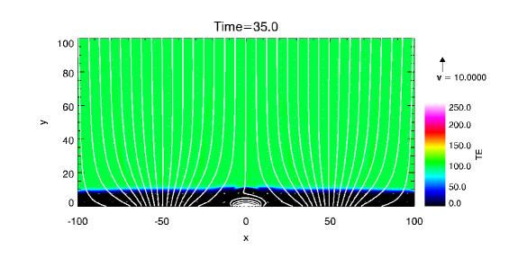
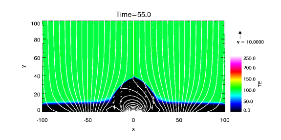
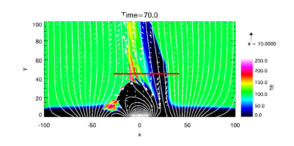
Figure 3: Temperature distributions (color scale), projected magnetic field (solid lines) and velocity field (vector arrows) at times 35 (upper panel), 55 (middle panel) and 70 (lower panel). The units of length, temperature, time and velocity are $301.6$ km, $10000$ K, $33.1$ s, $9.09$ km s^-1, respectively.

The reconnection rate and the one dimensional (1D) distributions of density, temperature and $y$-component of the velocity along the red line in Figure 3 are illustrated in Figure 4. The reconnection rate is calculated by the ratio of the inflow speed ($V_{in}$) and the local Alfvén speed ($V_{A}$). Both two speeds are measured around the current sheet. The reconnection rate reaches the maximum around time=$70$ (38 minutes) and its value is about 0.09 that is within the value of 0.01 - 0.1 predicted by Petschek (1964). The high reconnection rate partly results from some small plasmoids ejections from the X-point, which may increase the reconnection rate (Shibata et al., 1995; Shibata, 1996). While after time=$76$, some numerical errors occur at the center of the EMF. Thus, the result after that time is unreliable although the reconnection rate increases again (see the upper left panel of Figure 4). A roughly estimated life time of this coronal microflare is about 12 minutes if we take the duration being from the beginning (time=$55$) to the ending (time=$75$) of the main reconnection. That is consistant with the observations values (10 - 30 minutes; Shimizu et al., 2002; Fang et al., 2006, 2010). The other three panels show one dimensional distributions of density, temperature and $y$-component velocity at time=$45$, respectively. As we mentioned above, a hot jet and a cold surge are formed in this case. The hot jet ($\sim 1.8\times 10^{6}$K) which originates from the reconnection region, is ejected to the higher corona with the velocity of $16$ (about 140 km s^-1), which corresponds to the observational EUV/SXR jet (Chae et al., 1999; Brosius & Holman, 2009). The denser cold surge ($\sim 10^{4}$ K and the density is two orders of magnitude larger than that of the hot jet), which is drawn to the corona by the hot jet. The cold surge falls to the lower atmosphere later with the speed of 3 ($\sim$ 30 km s^-1). This process is similar to the observational H$\alpha$/Ca surge (Chae et al., 1999). The estimated size of the EUV/SXR or H$\alpha$ bright point in our simulation is about $50$ from $x=-40$ to $10$ ($\sim 15000$ km, i.e. $\sim 20$ arcsec).

Figure 4: The upper left panel shows the magnetic reconnection rate using the ratio between the inflow and Alfvén speeds. Three vertical dashed lines in this panel outline the times used in Figure 3. The other three panels are one dimensional distributions of density (RO), temperature (TE) and $y$-component velocity (VY) along the solid red line shown in the lower panel of Figure 3. The horizontal dashed lines show the initial values while the vertical lines indicate the boundary between the hot and cold jets in these three panels. The density, length, temperature, time and velocity units are $2.56\times 10^{-8}$ kg m^-3, $301.6$ km, $10000$ K, $33.1$ s and $9.09$ km s^-1, respectively.

3.2 Chromospheric Microflare

In this case, the strength and half width of the EMF are set to be $B_{e}=12$ ($200$ G), $\eta_{max}=0.1$ and $r_{0}=6$ ($\sim 1800$ km). Compared the coronal case, the reconnection process is similar but the simulation result is totally differenct, since the coronal magnetic field prevents the weak EMF emerging to the height as high as the coronal one. Therefore, the magnetic field accumulated in the chromosphere until the local current density exceeds the threshold ($j_{c}=10$, the same as the coronal case). Finally, we got the chromospheric microflare resulting from a fast reconnection mainly in the chromosphere and partly in the transition region. The result of this chromospheric microflare is given by three snapshots in Figure 5. Similar to Figure 3, the three panels correspond to the times before the reconnection, the time when reconnection rate is increasing, and the time when the reconnection rate reaches to the maximum (as shown by the upper left panel of Figure 6), respectively. In this case, the reconnection occurs at the chromosphere and the size of this microflare is about 15 from $x=-10$ to $5$ ($\sim 4500$ km, i.e. $\sim 6$ arcsec). There is no obvious reconnection jets ejected into the corona and we only obtain some temperature enhancements in the chromosphere and partly in the transition region.

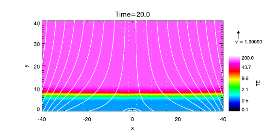
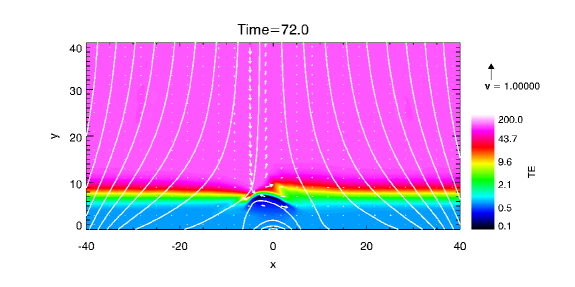
Figure 5: Temperature distributions (color scale), projected magnetic field (solid lines) and velocity field (vector arrows) at time 20 (upper panel), 40 (middle panel) and 72 (lower panel). The units of length, temperature, time and velocity are $301.6$ km, $10000$ K, $33.1$ s and $9.09$ km s^-1, respectively.

The reconnection rate and the one dimensional (1D) distribution of temperature along the red line in Figure 5 are illustrated in Figure 6. The physical process is much simpler than the corona case. As the reconnection occurs in the dense chromosphere, it is very hard to heat the plasma to a very high temperature. The right panel of Figure 6 is the temperature distribution at the the height of 1500 km. The inital value of the temperature is 0.64 (6400 K) and the temperature enhancement is about 800 K at this layer. The low temperature region is due to the expansion of the EMF. As we know, the plasma satisfies the frozen-in condition in the solar atmosphere without the resistivity. Therefore, the plasma of the lower atmosphere is dominanted by the strong magnetic field and finally such an adiabatic expansion will reduce the temperature. The low adiabatic index ($\gamma=1.1$ in our simulations) can decrease such an effect, which also makes the simulated system more similar as an isothermal process. Although we can see two regions where the temperature is increased as seen in Figure 6, they are not be observed as two H$\alpha$ bright points since the hot region is a shell covering the EMF as seen from the lower panel of Figure 5. That is to say, we can only observe one H$\alpha$ bright point if the line of sight is along the $y$-axis. The size of this bright point is about 15 from $x=-10$ to $5$ ($\sim 4500$ km, i.e. $\sim 6$ arcsec). There is no obvious temperature enhancement in the corona. Thus this case can explain the microflares with only H$\alpha$ emssion. The inflow (downward) speed in the lower panel of Figure 5 is about 6 km s^-1 which may be observed as a redshifted Doppler velocity in coronal lines. The outflow velocity of the reconnection flow in the chromosphere is about 20 km s^-1, but the direction of this outflow is redirected by background canopy-type field. Eventually, this coronal outflow ($\sim 4$ km s^-1) moves upward next to the downward inflow as shown by the lower panel of Figure 5.

Figure 6: The left panel shows the magnetic reconnection rate using the ratio between the inflow and Alfvén speed. Three vertical dashed lines in this panel outline the times used in Figure 5. The other panel are one dimensional distributions of temperature (TE) along the solid red line shown in the lower panel of Figure 5. The horizontal dashed lines show the initial value. The length, temperature and time units are $301.6$ km, $10000$ K and $33.1$ s, respectively.

3.3 Parameter Dependence

So far we have simulated one coronal case and one chromospheric case. An important question is which parameters determine whether reconnection happens in the corona or in the chromosphere when an EMF appears. In this subsection, we study three parameters, i.e., the strength of the EMF ($B_{e}$), the maximum value of resistivity ($\eta_{max}$), and the half width of EMF ($r_{0}$). In order to understand the effects of different parameters, we perform extensive simulations by changing one parameter with others being fixed.

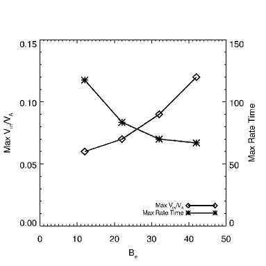
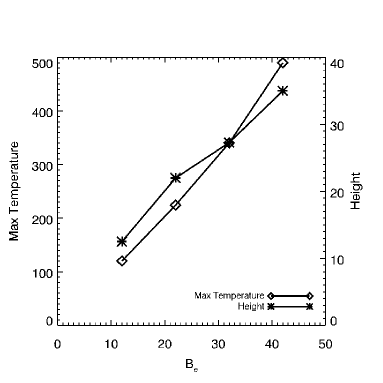
Figure 7: The left panel shows the dependence of Max $V_{in}/V_{A}$ (maximum magnetic reconnection rate) and Max Rate Time (the time when the reconnection rate reaches the maximum) on different strength of the EMF magnetic field. The right panel depicts the dependence of Max Temperature (the maximum temperature at the Max Rate Time ) and Height (the height of current sheet center at the Max Rate Time ) on different strengths of EMF magnetic field. The length, temperature, time and magnetic field units are $301.6$ km, $10000$ K, $33.1$ s and $16.3$ G, respectively.

Figure 7 shows the dependence of the reconnection process on different strengths of the EMF magnetic field. Four values of $B_{e}$ are studied, i.e., $B_{e}=12,22,32$ and $42$, whereas the other two parameters are fixed, i.e., $\eta_{max}=0.1$ and $r_{0}=8$. With the increasing of the strength of the EMF, the magnetic reconnection rate can reach the maximum much faster and the maximum reconnection rate becomes larger and larger when we set a stronger initial magnetic field. The right panel shows how the maximum temperature and the height of the current sheet center change with the strength of EMF magnetic field. The Max Temperature and Height is very sensitive to the parameter $B_{e}$. A stronger EMF can result to a higher altitude which can generate a stronger current density. Thus, it is easy to trigger the reconnection at an earlier time. The reconnection is faster and the outflow is hotter than a weak EMF. When we set $B_{e}=12$, we find that the height is 12.5 (3750 km), which is located nearly above the transition region. If we keep reducing the value $B_{e}$, the reconnection will occur in the chromosphere.

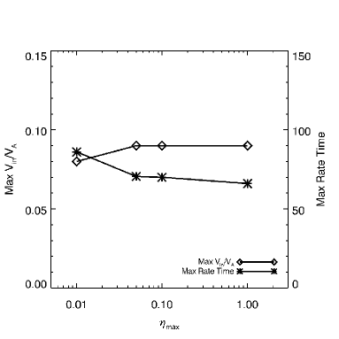
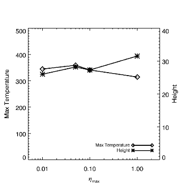
Figure 8: The left panel shows the dependence of Max $V_{in}/V_{A}$ and Max Rate Time on different maximum values of resistivity ($\eta_{max}$). The right panel depicts the dependence of Max Temperature and Height on different maximum values of resistivity ($\eta_{max}$). The length, temperature, time and resistivity units are $301.6$ km, $10000$ K, $33.1$ s and 3445.1 $\Omega$ m, respectively.

Figure 8 shows the dependence of various quantities on different values of maximum resistivity ($\eta_{max}$). Four different values are selected, i.e., $\eta_{max}=0.01,0.05,0.1$ and $1.0$. The other two parameters are fixed, i.e. $B_{e}=32$ and $r_{0}=8$. We got the similar results as described in our previous paper (Jiang et al., 2010). The variation of the resistivity value does not change the results too much. The reconnections almost occur around the heigh of 28 (8500 km) and the temperature enhancement at such a height is about 350 ($3.5\times 10^{6}$).

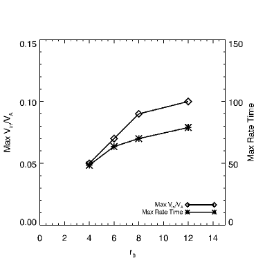
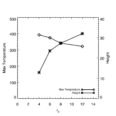
Figure 9: The left panel shows the dependence of Max $V_{in}/V_{A}$ and Max Rate Time on different half width ($r_{0}$) of the EMF. The right panel depicts the dependence of Max Temperature and Height on different half width ($r_{0}$) of the EMF. The length, temperature, time and length units are $301.6$ km, $10000$ K, $33.1$ s and $301.6$ km, respectively.

The dependence on different half widths ($r_{0}=4,6,8$ and $12$) are depicted in Figure 9. The other two fixed parameters are $B_{e}=32$ and $\eta_{max}=0.1$. From the reconnection start time to the maximum time, a bigger EMF can rise to a higher altitude. We know that in the higher altitude the plasma $\beta$ is lower, thus the magnetic reconnection can be very fast with the same resistivity. At the same time, the strength of the magnetic field of EMF becomes weaker and weaker after expanding to such a long distance, so the temperature enhancement becomes smaller and smaller as indicated by Figure 7. Therefore, the left panel of Figure 9 shows the reconnection rate and the reconnection duration increase with the increasing half width of the EMF. In the right panel, we find that the height of X-point is also sensitive to the size of the EMF. Combining the small magnetic strength of the EMF, we can get the result of chromospheric microflare as described in Section 3.2.

4 DISCUSSION AND SUMMARY

In this paper, we simulate the microflares produced by EMFs. The EMFs with different strength and size lead to different results. Two types of the microflares in our simulations, i.e., of coronal origin and of chromospheric origin, can be illustrated by the cartoon in Figure 10. According to our simulations, small microflares with weak Doppler velocities and only H$\alpha$ emissions are most likely due to the reconnection in the lower solar atmosphere (for instance, the chromosphere or photosphere). However, big microflares with obvious Doppler velocities and emissions in both low and high temperature wavelengthes (H$\alpha$ and EUV/SXR) originate from the reconnection in the corona. This model is similar to the unified model of Shibata (1996); Shibata et al. (2007) and Chen et al. (1999) in the sense that the different behaviors of eruptions are determined by the different height of the magnetic reconnection. According to the result in this paper, the strength and the size of the EMF determines whether the microflare is of coronal origin or of chromospheric origin when the EMF emerges from the center of a supergranule, probably dragged by the convective upflow. Of course, EMFs may also appear at other sites of a supergranule, which would also affect the height of the reconnection site.

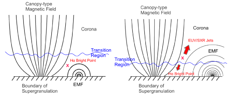
Figure 10: The cartoon shows the basic physical process of our simulated two types of microflares, i.e. of chromospheric and coronal origins.

As mentioned in Section 3.1, we find some plasmoids in our simulations. Figure 11 shows the current density distribution of a small region [-35, 0] $\times$ [10, 45] in Figure 3. From both the temperature and current density distributions (Figure 3 and 11), we can see a plasmoid is formed at the center of the current sheet. The ejection of the plasmoid can increase the magnetic reconnection rate temporarily (Shibata et al., 1995; Shibata, 1996; Shen et al., 2011). In the reconnection process, the plasmoids are generated one by one, therefore we can see some oscillations of the reconnection rate in Figure 4. However, for the chromospheric case, the Alfvén speed is much smaller than the coronal one, which leads to a smaller magnetic Reynolds number. Thus, similar to the results presented by Shen et al. (2011), there is no plasmoid produced in the chromospheric case. The corresponding reconnection rate in Figure 6 also shows less oscillations. In the coronal case, as the reconnection occurs in the corona, both hot jets and cold surges are ejected. No doubt that the EUV/SXR emissions from the hot jet will be observed first, whereas H$\alpha$/Ca bright points and surges appear later. If we take the temperature response at the height of 1500 km, which is the H$\alpha$ formation height (Vernazza et al., 1981), the roughly calculated time delay between the EUV/SXR and H$\alpha$ emissions is about 3–5 minutes, which is comparable to the observations (Zhang et al., 2012). We have to mention that the temperature enhancement and the time delay can be more realistic if we include the thermal conduction, radiation, the high energe particles (non-thermal electrons and ions), and the effect of partially ionised plasma. For simplicity and for the sake to see how emerging flux with different sizes and strengths influencesthe reconnection, we kept the threshold of the current density $j_{c}$ in the anomalous resisitivity in Eq. (8) to be constant. In reality, the threshold of $j_{c}$ in the chromosphere might be higher because of its high plasma density. In order to see how $j_{c}$ would change the reconnection process, we performed other numerical experiments with higher $j_{c}$ in the chromosphere, and it is found that the basic results are the same, the main difference is that the commencement of reconnection is postponed only for the case that the current sheet located at the chromosphere, as demonstrated by Yokoyama & Shibata (1994).

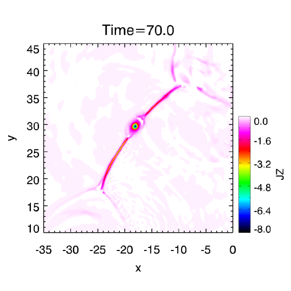
Figure 11: A amplified view of $z$-component current density (JZ) distribution of the conoral case at the time 70. The overall view of temperature distribution is shown by the bottom panel of Figure 3 at the same time. The range of this box is [-35, 0] $\times$ [10, 45], in which a plasmoid in the center of the current sheet is clearly seen.

In summary, we successfully simulated the coronal and chromospheric microflares by using MHD simulations with a canopy-type magnteic configuration. The different observational behaviors between coronal microflares and chromospheric ones are due to the height of magnetic reconnection, which is determined by the size of the emerging flux, i.e., smaller emerging flux produces chromospheric microflares and larger emerging flux produces coronal microflares. Correspondingly, the resulting microflares have different sizes. In the case of coronal origin, the sizes of the simulated microflares are $11000-16000$ km, i.e., $15-22$″, which correspond to big microflares. We find a hot jet ($\sim$$1.8\times 10^{6}$ K for the typical case), which should be relates to the observational EUV/SXR jet, and a cold jet ($\sim$$10^{4}$ K for the typical case), which corresponds to the observational H$\alpha$/Ca surge or brightening. Some plasmoids generated at the center of the current sheet are ejected, which can increase the magnetic reconnection rate. In the case of chromospheric origin, the sizes of the microflares are $4200-4500$ km, i.e., $\sim$6$\arcsec$, which correspond to relatively small microflares. As the reconnection occurs in the chromosphere, only the H$\alpha$/Ca brightenings show up in this case, where no significant SXR brightening and no plasmoids are produced in this case. The parameter survey qualitatively shows that the size and strength of the EMF are the key parameters which determine the height of the reconnection X-point. For some typical values, we can get the reconnection either in the corona or in the chromosphere. The parameter $\eta_{max}$ has little effect on the final results.

This paper deals with the microflares related to EMFs. It should be mentioned that some microflares are due to other mechanisms, e.g., the reconnection between the MMFs (Harvey & Harvey, 1973) and the pre-existing magnetic field. Priest et al. (1994) proposed a canceling magnetic features model. Browning et al. (2008) performed 3D MHD simulations to study the role of kink instability in the magnetic energy releas process, which may also lead to microflares. It is also noticed that the simulated emerging flux in this paper does not include the twisted field, which is required for the emerging flux to survive the subsurface convection (see Babcock, 1961; Piddington, 1975; Fan, 2009, and references therein), e.g., Murray & Hood (2008) found that the tension force of twisted tube plays a key role in determining whether the flux can successfully emerge to the upper solar atmosphere in 3D numerical experiments. In the 2D coronal simulations, the twisted field can be easily considered by including $B_{z}$, which would not change the results greatly. Moreover, a single-fluid model for the solar atmosphere was adopted in this paper for simplicity. In reality, the chromosphere, especially the lower part, is weakly-ionzed, and partial ionization should be considered, which would lead to strong anisotropic Cowling resistivity (Cowling, T. G., 1957; Khodachenko et al., 2004; Leake & Arber, 2006), ambipolar diffusion (Vishniac & Lazarian, 1999; Soler et al., 2009; Singh et al., 2011). Moreover, the ionization of neutral atoms would consume a significant part of the released energy in the magnetic reconnection (Chen et al., 2001; Jiang et al., 2010).

References

- Archontis Török (2008) Archontis, V., Török, T. 2008, A&A, 492, L35
- Archontis & Hood (2009) Archontis, V., & Hood, A. W. 2009, A&A, 508, 1469
- Babcock (1961) Babcock, H. W. 1961, ApJ, 133, 572
- Berger & Oliger (1984) Berger, M. J., & Oliger, J. 1984, J. Comput. Phys., 53, 484
- Berger & Colella (1989) Berger, M. J., & Colella, P. 1989, J. Comput. Phys., 82, 64
- Brackbill & Barnes (1980) Brackbill, J. U., & Barnes, D. C. 1980, Journal of Computational Physics, 3, 426
- Brosius & Holman (2009) Brosius, J. W., & Holman, G. D. 2009, ApJ, 692, 492
- Browning et al. (2008) Browning, P. K., Gerrard, C., Hood, A. W., Kevis, R., & van der Linden, R. A. M. 2008, A&A, 485, 837
- Chae et al. (1999) Chae, J., Qiu, J., Wang, H., & Goode, P. R. 1999, ApJ, 513, L75
- Chen et al. (1999) Chen, P. F., Fang, C., Ding, M. D., & Tang, Y. H. 1999, ApJ, 520, 853
- Chen & Shibata (2000) Chen, P.-F., & Shibata, K. 2000, ApJ, 545, 524
- Chen et al. (2001) Chen, P.-F., Fang, C., & Ding, M.-D. D. 2001, ChJAA, 1, 176
- Chen & Ding (2010) Chen, F., & Ding, M.-D. 2010, ApJ, 724, 640
- Cowling, T. G. (1957) Cowling, T. G., Magnetohydrodynamics (New York: Interscience), 1957
- Dedner et al. (2002) Dedner et al. 2002, J. Comput. Phys., 175, 645
- Ding et al. (2010) Ding, J. Y., Madjarska, M. S., Doyle, J. G., & Lu, Q. M. 2010, A&A, 510, A111
- Ding et al. (2011) Ding, J. Y., Madjarska, M. S., Doyle, J. G., Lu, Q. M., Vanninathan, K., & Huang, Z. 2011, A&A, 535, A95
- Emslie & Noyes (1978) Emslie, A. G., & Noyes, R. W. 1978, Sol. Phys., 57, 373
- Evans & Hawley (1988) Evans, C. R., & Hawley, J. F. 1988, ApJ, 332, 659
- Fan (2001) Fan, Y. 2001, ApJ, 554, L111
- Fan (2009) Fan, Y. 2009, Living Reviews in Solar Physics, 6, 4
- Fang et al. (2006) Fang, C., Tang, Y.-H., & Xu, Z. 2006, ChJAA, 6, 597
- Fang et al. (2010) Fang, C., P.-F. Chen, R.-L. Jiang & Y.-H. Tang 2010, RAA, 10, 83
- Forbes & Priest (1984) Forbes, T. G., & Priest, E. R. 1984, Sol. Phys., 94, 315
- Gabriel (1976) Gabriel, A. H. 1976, Royal Society of London Philosophical Transactions Series A, 281, 339
- Galsgaard et al. (2005) Galsgaard, K., Moreno-Insertis, F., Archontis, V., & Hood, A. 2005, ApJ, 618, L153
- Galsgaard et al. (2007) Galsgaard, K., Archontis, V., Moreno-Insertis, F., & Hood, A. W. 2007, ApJ, 666, 516
- Gary & Zirin (1988) Gary, D. E., & Zirin, H. 1988, ApJ, 329, 991
- Gary et al. (1997) Gary, D. E., Hartl, M. D., & Shimizu, T. 1997, ApJ, 477, 958
- Giovanelli (1980) Giovanelli, R. G. 1980, Sol. Phys., 68, 49
- Giovanelli (1982) Giovanelli, R. G. 1982, Sol. Phys., 80, 21
- Gopalswamy et al. (1994) Gopalswamy, N., Payne, T. E. W., Schmahl, E. J., Kundu, M. R., Lemen, J. R., Strong, K. T., Canfield, R. C., & de La Beaujardiere, J. 1994, ApJ, 437, 522
- Golub et al. (1974) Golub, L., Krieger, A. S., Silk, J. K., Timothy, A. F., & Vaiana, G. S. 1974, ApJ, 189, L93
- Golub et al. (1977) Golub, L., Krieger, A. S., Harvey, J. W., & Vaiana, G. S. 1977, Sol. Phys., 53, 111
- Harvey & Harvey (1973) Harvey, K., & Harvey, J. 1973, Sol. Phys., 28, 61
- Harten (1997) Harten, A. 1997, J. Comput. Phys., 135, 260
- Hood et al. (2009) Hood, A. W., Archontis, V., Galsgaard, K., & Moreno-Insertis, F. 2009, A&A, 503, 999
- Horiuchi et al. (1988) Horiuchi, T., Matsumoto, R., Hanawa, T., & Shibata, K. 1988, PASJ, 40, 147
- Isobe et al. (2005) Isobe, H., Miyagoshi, T., Shibata, K., & Yokoyama, T. 2005, Nature, 434, 478
- Isobe et al. (2007) Isobe, H., Tripathi, D., & Archontis, V. 2007, ApJ, 657, L53
- Jess et al. (2010) Jess, D. B., Mathioudakis, M., Browning, P. K., Crockett, P. J., & Keenan, F. P. 2010, ApJ, 712, L111
- Jiang & Wu (1999) Jiang, G.-S., & Wu, C.-C. 1999, J. Comput. Phys., 150, 561
- Jiang et al. (2010) Jiang, R. L., Fang, C., & Chen, P. F. 2010, ApJ, 710, 1387
- Jiang et al. (2012) Jiang, R.-L., Fang, C., Chen, P.-F., 2012, Comput. Phys. Comm., 183, 1617
- Jin et al. (1996) Jin, S.-P., Inhester, B., & Innes, D. 1996, Sol. Phys., 168, 279
- Kano et al. (2010) Kano, R., Shimizu, T., & Tarbell, T. D. 2010, ApJ, 720, 1136
- Khodachenko et al. (2004) Khodachenko, M. L., Arber, T. D., Rucker, H. O., & Hanslmeier, A. 2004, A&A, 422, 1073
- Leake & Arber (2006) Leake, J. E., & Arber, T. D. 2006, A&A, 450, 805
- Lin et al. (1984) Lin, R. P., Schwartz, R. A., Kane, S. R., Pelling, R. M., & Hurley, K. C. 1984, ApJ, 283, 421
- Magara (2001) Magara, T. 2001, ApJ, 549, 608
- Manchester et al. (2004) Manchester, W., IV, Gombosi, T., DeZeeuw, D., & Fan, Y. 2004, ApJ, 610, 588
- Martínez-Sykora et al. (2011) Martínez-Sykora, J., Hansteen, V., & Moreno-Insertis, F. 2011, ApJ, 736, 9
- Matsumoto et al. (1988) Matsumoto, R., Horiuchi, T., Shibata, K., & Hanawa, T. 1988, PASJ, 40, 171
- Matsumoto (2007) Matsumoto, T. 2007, PASJ, 59, 905
- Murray & Hood (2008) Murray, M. J., & Hood, A. W. 2008, A&A, 479, 567
- Ning (2008) Ning, Z. 2008, ApJ, 686, 674
- Nishizuka et al. (2008) Nishizuka, N., Shimizu, M., Nakamura, T., Otsuji, K., Okamoto, T. J., Katsukawa, Y., & Shibata, K. 2008, ApJ, 683, L83
- Parker (1966) Parker, E. N. 1966, ApJ, 145, 811
- Petschek (1964) Petschek, H. E., 1964, in physics of Solar Flares, ed. W. N. Hess, NASA SP-50, Washington, DC, p. 425
- Piddington (1975) Piddington, J. H. 1975, Ap&SS, 34, 347
- Porter et al. (1984) Porter, J. G., Toomre, J., & Gebbie, K. B. 1984, ApJ, 283, 879
- Powell et al. (1999) Powell, K. G., et al. 1999, J. Comput. Phys., 154, 284
- Priest et al. (1994) Priest, E. R., Parnell, C. E., & Martin, S. F. 1994, ApJ, 427, 459
- Qiu et al. (2004) Qiu, J., Liu, C., Gary,D. E., Nita, G. M., & Wang, H. 2004, ApJ, 612, 530
- Schmieder et al. (1997) Schmieder, B., Aulanier, G., Demoulin, P., van Driel-Gesztelyi, L., Roudier, T., Nitta, N., & Cauzzi, G. 1997, A&A, 325, 1213
- Shen et al. (2011) Shen, C., Lin, J., & Murphy, N. A. 2011, ApJ, 737, 14
- Shibata et al. (1989a) Shibata, K., Tajima, T., Matsumoto, R., Horiuchi, T., Hanawa, T., Rosner, R., & Uchida, Y. 1989a, ApJ, 338, 471
- Shibata et al. (1989b) Shibata, K., Tajima, T., Steinolfson, R. S., & Matsumoto, R. 1989b, ApJ, 345, 584
- Shibata et al. (1995) Shibata, K., Masuda, S., Shimojo, M., Hara, H., Yokoyama, T., Tsuneta, S., Kosugi, T., & Ogawara, Y. 1995, ApJ, 451, L83
- Shibata (1996) Shibata, K. 1996, Advances in Space Research, 17, 9
- Shibata et al. (2007) Shibata, K., et al. 2007, Science, 318, 1591
- Shimizu et al. (2002) Shimizu, T., Shine, R. A., Title, A. M., Tarbell, T. D., & Frank, Z. 2002, ApJ, 574, 1074
- Singh et al. (2011) Singh, K. A. P., Shibata, K., Nishizuka, N., & Isobe, H. 2011, Plasma Physics, 18, 111210
- Smith & Smith (1963) Smith, H. J., & Smith, E. V. P. 1963, New York, Macmillan [1963]
- Soler et al. (2009) Soler, R., Oliver, R., & Ballester, J. L. 2009, ApJ, 699, 1553
- Stone & Norman (1992) Stone, J. M., & Norman, M. L. 1992, ApJS, 80, 791
- Tóth (2000) Tóth, G. 2000, J. Comput. Phys., 161, 605
- Svestka (1976) Svestka Z., Solar Flares, 1976, Dordrecht: D.Reidel Publ. Co., Holland.
- Tandberg-Hanssen & Emslie (1988) Tandberg-Hanssen E., Emslie A. G., The physics of solar flares, 1988, Cambridge: Cambridge University Press
- Tang et al. (2000) Tang, Y. H., Li, Y. N., Fang, C., Aulanier, G., Schmieder, B., Demoulin, P., & Sakurai, T. 2000, ApJ, 534, 482
- Török et al. (2009) Török, T., Aulanier, G., Schmieder, B., Reeves, K. K., & Golub, L. 2009, ApJ, 704, 485
- Toth & Odstrčil (1996) Tóth, G., & Odstrčil, D. 1996, J. Comput. Phys., 128, 82
- Ugai (1985) Ugai, M. 1985, Plasma Phys. Controlled Fusion, 27, 1183
- Vernazza et al. (1981) Vernazza, J. E., Avrett, E. H., & Loeser, R. 1981, ApJS, 45, 635
- Vishniac & Lazarian (1999) Vishniac, E. T., & Lazarian, A. 1999, ApJ, 511, 193
- Xu et al. (2011) Xu, X.-Y., Fang, C., Ding, M.-D., & Gao, D.-H. 2011, Research in Astronomy and Astrophysics, 11, 225
- Yokoyama & Shibata (1994) Yokoyama, T., & Shibata, K. 1994, ApJ, 436, L197
- Yokoyama & Shibata (1995) Yokoyama, T., & Shibata, K. 1995, Nature, 375, 42
- Yokoyama & Shibata (2001) Yokoyama, T., & Shibata, K. 2001, ApJ, 549, 1160
- Yu & Liu (2001) Yu, H., & Liu, Y.-P. 2001, J. Comput. Phys., 173, 1
- Zhang et al. (2012) Zhang, P., Zhang Q.-M. & Fang, C. 2012, Science China, 55, 907