A new MHD code with adaptive mesh refinement and parallelization for astrophysics

Abstract

A new code, named MAP, is written in FORTRAN language for magnetohydrodynamics (MHD) calculation with the adaptive mesh refinement (AMR) and Message Passing Interface (MPI) parallelization. There are several optional numerical schemes for computing the MHD part, namely, modified Mac Cormack Scheme (MMC), Lax-Fridrichs scheme (LF) and weighted essentially non-oscillatory (WENO) scheme. All of them are second order, two-step, component-wise schemes for hyperbolic conservative equations. The total variation diminishing (TVD) limiters and approximate Riemann solvers are also equipped. A high resolution can be achieved by the hierarchical block-structured AMR mesh. We use the extended generalized Lagrange multiplier (EGLM) MHD equations to reduce the non-divergence free error produced by the scheme in the magnetic induction equation. The numerical algorithms for the non-ideal terms, e.g., the resistivity and the thermal conduction, are also equipped in the MAP code. The details of the AMR and MPI algorithms are described in the paper.

1 Introduction

The adaptive mesh refinement (AMR) algorithm was firstly proposed by Berger and Oliger [1] and Berger and Colella [2], which can recursively create finer overlapping meshes to a given accuracy based on the Richardson error estimation. Using AMR, one can resolve a very small region in a very large scale simulation, for instance, the simulation of the propagation of solar wind from the Sun to the Earth, the protostellar collapse in the processes of star formation, the very thin current sheets in magnetic reconnection, and so on. There are two advantages comparing to uniform grid: AMR is very fast and effective to get a global high resolution; it can also refine any part of the computational box.

The preliminary block structured AMR method [1, 2] is not so easy to extend to multiprocessor calculation because the sizes of the blocks in the AMR hierarchical grid are different which generate difficulty in load balance between different processors, although the arbitrary shapes of the blocks can get a flexible and efficient memory usage. The data blocks, which are the subgrids of the base grid, allow to have arbitrary shapes and can merge with other blocks at the same level. In order to overcome this drawback, a simple approach was developed by DeZeeuw and Powell [3]. The basic idea is to build a hierachical binarytree for one dimension (1D), quadtree for two dimension (2D) and octree for three dimension (3D). These tree structures contain the necessary information between the parent blocks, child blocks and neighbor blocks, which can be used to update the block data from the finer blocks or exchange boundary data from the neighbor blocks. All blocks in all refinement levels have the exact same shape and can be easily parallelled using the Morton space filling curve (Z-curve [4]), Hilbert space filling curve (H-curve [5]), or other curves.

There are many existing AMR codes including FLASH [6], AMRVAC [7], PLUTO [8], SFUMATO [9], NIRVANA [10, 11], RAMSES [12], RIEMANN [13], CRASH [14], CHARM [15], CASTRO [16, 17] and so on. Some of them, e.g. FLASH and PLUTO, are using the AMR library like PARAMESH [18] toolkit, CHOMBO library [19] or BoxLib library [20]. Other codes, however, developed their own AMR algorithms for better performance. Our code, named as MAP (MHD code with adaptive mesh refinement and parallelization for astrophysics), was also designed with the same considerations. Besides, being easy to use and modify is another purpose. In the developing process, we learn much experience from these pioneers’ papers, for instance, the block structured idea from Berger and Colella [2] and DeZeeuw and Powell [3], the error estimation method from Ziegler [11], the file management method from the code AMRVAC developed by Keppens et al. [7] and CANS (Coordinated Astronomical Numerical Softwares).

The major difference between our code and most of the existing codes is that we use the extended generalized Lagrange multiplier (EGLM) MHD equations which have one more variable and one more equation representing the damping and transfer of the non-divergence free error as described by Dedner et al. [21]. The method of constrained transport (CT) [22] is not included in our MAP code, although it is almost perfect to control the divergence free condition to the machine round-off error. The reasons are: (1) it is complicated in an AMR code as it requires a staggered mesh; (2) additional variables have to be allocated for the cell center value of magnetic field, and the boundary data exchanging process is complex which takes much longer time than the unstraggered grids; (3) it requires a strict divergence free boundary condition, because CT can only guarantee the zero divergence condition from the old time to new time. When we use a rapidly-changing boundary, for instance, an emerging flux boundary, it will inevitably produce non-divergence free magnetic field. In this case, the CT method may not be a good choice. There are several numerical schemes optionally for computing the EGLM-MHD equations, namely, modified Mac Cormack Scheme (MMC) [23], Lax-Fridrichs (LF) [24] and weighted essentially non-oscillatory (WENO) [25]. Since all of them are second-order, two-step, component-wise schemes for hyperbolic conservation laws, the code is fast, effective and lightweight. One can easily understand what is going on in the FORTRAN codes of the three schemes according to the formulae described in Section 3. It is also convenient to modify the code or even add a new MHD solver. This is another feature of our code. The three schemes have their own special implements. The first two schemes, i.e. the MMC and LF schemes, are equipped with the total variation diminishing [TVD 26] limiters, while the latter two, i.e. the LF and WENO, are implemented with the approximate Riemann solvers. In MHD, the exact solver for Riemann problem is too complex and time consuming, thus only the simple solver like nonlinear Harten-Lax-van Leer Contact (HLLC) [27], Harten-Lax-van Leer Discontinuities (HLLD) [28] and Roe linear solver [29, 30] are adopted in the code MAP. There are several reasons for us not using higher-resolution numerical schemes (for instance, the piecewise parabolic method (PPM) by Colella [31], Dai and Woodward [32] or corner transport upwind PPM (CTU-PPM) by Gardiner and Stone [33, 34] or 5th order WENO by Jiang and Shu [35], Jiang and Wu [25]): (1) the lack in accuracy can be compensated by the hierarchical block-structured AMR algorithm; (2) the accuracy of many parts of the equations like the thermal conduction and the resistivity, divergence cleanance method, as well as AMR reflux and interpolation method, can not always guarantee a high-order precision, which would lead to a poor global accuracy; (3) the high-order method is complex and time consuming.

Our current MAP code is based only on the Cartesian coordinates, and the extension to cylindrical and spherical grids will be conducted in the next version. The other improvements like finite difference (FD) and finite volume (FC) schemes, the radiation cooling for both optically thin and thick situations, and the relativistic MHD module are in consideration too. The AMR strategy for high-order FD and FV schemes are almost the same except the algorithm of boundary reflux between coarse and fine meshes, interpolation from parent blocks to child blocks and update parent blocks from child blocks at the new time. For a high-order FD scheme, if we use the same procedure as in FV, the scheme may lose some conservation and accuracy according to our practical experience. That is our additional reason for using only second-order schemes.

The organization of this paper is as follows: Section 2 introduces the basic EGLM-MHD equations for the divergence clean in our code; Section 3 describes the numerical schemes for solving the EGLM-MHD equations including the resistivity and thermal conduction; The detailed AMR algorithm with MPI is given in Section 4; Some numerical tests in 1D, 2D and 3D are presented in Section 5; Finally, we give a summary in Section 6.

2 EGLM-MHD equation

The dimensionless MHD equations with gravity, resistivity and thermal conduction included are given in conservative form as follows:

$$\frac{\partial\rho}{\partial t}+\nabla\cdot\left(\rho\mathbf{v}\right)=0\,\,,$$ (1)

$$\frac{\partial\left(\rho\mathbf{v}\right)}{\partial t}+\nabla\cdot\left(\left(p+\frac{1}{2}{B}^{2}\right)\mathbf{I}+\rho\mathbf{v}\mathbf{v}-\mathbf{B}\mathbf{B}\right)=\rho\mathbf{g}\,\,,$$ (2)

$$\frac{\partial\mathbf{B}}{\partial t}+\nabla\cdot\left(\mathbf{v}\mathbf{B}-\mathbf{B}\mathbf{v}\right)=-\nabla\times\left(\eta\nabla\times\mathbf{B}\right)\,\,,$$ (3)

$$\frac{\partial e}{\partial t}+\nabla\cdot\left(\mathbf{v}\left(e+\frac{1}{2}{B}^{2}+p\right)-\mathbf{B}\left(\mathbf{B}\cdot\mathbf{v}\right)\right)=-\nabla\cdot\left(\left(\eta\nabla\times\mathbf{B}\right)\times\mathbf{B}\right)+\nabla\cdot\left(\kappa\nabla T\right)+\rho\mathbf{g}\cdot\mathbf{v}\,\,,$$ (4)

here, eight independent conserved variables are the density ($\rho$), momentum ($\rho v_{x}$, $\rho v_{y}$, $\rho v_{z}$), magnetic field ($B_{x}$, $B_{y}$, $B_{z}$), and total energy density ($e$). The expression of the total energy density is $e=p/(\gamma-1)+\rho v^{2}/2+B^{2}/2$. The pressure $p$ and temperature $T$ are dependent on the eight conserved variables, $\mathbf{g}$ is the gravity vector, and $\eta$ the magnetic resistivity coefficient, and $\kappa$ is the thermal conductivity coefficient. It is noted that $\kappa$ is not always a constant. It may relate to the local temperature value with the form $\kappa_{0}T^{5/2}$ (here $\kappa_{0}$ is another parameter for describing the conductivity). This thermal flux may associate with the direction of the magnetic field, the direction of this thermal flux may change to $(\mathbf{B}\cdot\nabla T)\mathbf{B}/B^{2}$ in some cases. Finally, a unity matrix $\mathbf{I}$ is involved for matrix operations. The vacuum permeability is omitted in this dimensionless MHD equation.

Almost all modern MHD codes have to face the problem of how to guarantee the divergence free requirement. Because of the discretization and numerical errors, the performance of the MHD code can be unphysical [36]. There are several ways to maintain $\nabla\cdot\mathbf{B}=0$ for MHD equations (1) - (4): (1) 8-wave formulation [37], (2) the CT method [22], (3) the projection scheme [36]. The 8-wave formulation can be easily implemented in a code by so-called “divergence source terms” without modifying the MHD solver. The numerical value of $\nabla\cdot\mathbf{B}$ can be controlled to a truncation error. The CT method is much robuster which can maintain the zero divergence condition to the machine round off error, but this method needs the staggered mesh which increase the difficulty in coding especially for AMR algorithm. The projection scheme introduces the Poisson equation to clean the numerical error of $\nabla\cdot\mathbf{B}$ which can preserve the conservative properties and the efficiency of the base scheme [38]. Another way to keep divergence-free condition is to modify the MHD equations (1) - (4) by using vector potential $\mathbf{A}$ instead of the magnetic field $\mathbf{B}$ as it was used in Chen et al. [39], or by using the vector magnetic potential or Euler poential. The advantage is that the divergence free condition is always satisfied, however, the MHD equation should be rewritten.

Recently, Dedner et al. [21] proposed the extended generalized Lagrange multiplier (EGLM) formulation of the MHD equations. This method uses two additional waves to transfer the numerical error of $\nabla\cdot\mathbf{B}$. Thus the local divergence error can be damped and passed out of the computational domain. It can also tansfer and damp the numerical error coming from the boundaries. As we described above, the rapidly-changing boundary will inevitably produce non-divergence free magnetic field. Actually, another method, the GLM-MHD system (i.e. mixed GLM scheme in Dedner’s paper), is also proposed in Dedner’s paper and Dedner et al. [21] themselves recommend GLM-MHD system rather than the EGLM-MHD system. The EGLM-MHD equations (5) - (9) is the GLM-MHD system extended by additional terms which may lead to some conservation loss. However, in some of our applications, we found that the GLM-MHD system works not so well as the EGLM-MHD system. Another reason, once we implement the EGLM-MHD, it is very easy to roll back to the GLM-MHD by disabling the additional source terms. Hence we adopted the EGLM-MHD equations of Dedner et al. [21] in our simulations. The EGLM-MHD equations with resistivity, thermal conduction and gravity included are given as follows:

$$\frac{\partial\rho}{\partial t}+\nabla\cdot\left(\rho\mathbf{v}\right)=0\,\,,$$ (5)

$$\frac{\partial\left(\rho\mathbf{v}\right)}{\partial t}+\nabla\cdot\left(\left(p+\frac{1}{2}{B}^{2}\right)\mathbf{I}+\rho\mathbf{v}\mathbf{v}-\mathbf{B}\mathbf{B}\right)=-\left(\nabla\cdot\mathbf{B}\right)\mathbf{B}+\rho\mathbf{g}\,\,,$$ (6)

$$\frac{\partial\mathbf{B}}{\partial t}+\nabla\cdot\left(\mathbf{v}\mathbf{B}-\mathbf{B}\mathbf{v}+\psi\mathbf{I}\right)=-\nabla\times\left(\eta\nabla\times\mathbf{B}\right)\,\,,$$ (7)

$$\frac{\partial e}{\partial t}+\nabla\cdot\left(\mathbf{v}\left(e+\frac{1}{2}{B}^{2}+p\right)-\mathbf{B}\left(\mathbf{B}\cdot\mathbf{v}\right)\right)=-\mathbf{B}\cdot\left(\nabla\psi\right)-\nabla\cdot\left(\left(\eta\nabla\times\mathbf{B}\right)\times\mathbf{B}\right)+\nabla\cdot\left(\kappa\nabla T\right)+\rho\mathbf{g}\cdot\mathbf{v}\,\,,$$ (8)

$$\frac{\partial\psi}{\partial t}+c_{h}^{2}\nabla\cdot\mathbf{B}=-\frac{c_{h}^{2}}{c_{p}^{2}}\psi\,\,,$$ (9)

where $\psi$ is a scalar potential propagating divergence error, $c_{h}$ the wave speed, and $c_{p}$ the damping rate of the wave [9, 21]. The other symbols have their normal meanings as in Eq. (1) - (4). As suggested in Dedner et al. [21], the expressions for $c_{h}$ and $c_{p}$ are

$$c_{h}=\frac{c_{cfl}}{\Delta t}\min(\Delta x,\Delta y,\Delta z)\,\,,$$ (10)

$$c_{p}=\sqrt{-\Delta t\frac{c_{h}^{2}}{\ln{c_{d}}}}\,\,.$$ (11)

where, $\Delta t$ is the time step, $\Delta x$, $\Delta y$ and $\Delta z$ are the space steps, $c_{cfl}$ is a safety coefficient less than 1. $c_{d}\in(0,1)$ is a problem dependent coefficient to decide the damping rate for the waves of divergence errors. The value of $c_{d}$ is 0.18 in most of our tests. We can see that $c_{h}$ and $c_{p}$ is not independent of the grid resolution and the scheme used. Hence we may have to adjust their values for different situations.

3 Numerical schemes

We use three different optional numerical schemes to solve the MHD part, i.e. MMC, LF and WENO as we mentioned above. In our calculations presented here, we mainly use the WENO scheme, the other two are used for comparison (see the accuracy test of these schemes in Section 5). Although the accuracy of all three schemes is not so high in both space and time, the advantage is that the coding is simple and the running speed is fast. In this section, we briefly review the three schemes by using the following 1D equation:

$$\frac{\partial u(x,t)}{\partial t}+\frac{\partial f\left(u(x,t)\right)}{\partial x}=0\,\,,$$ (12)

here $u(x,t)$ represents the eight conserved variables ($\rho$, $\rho v_{x}$, $\rho v_{y}$, $\rho v_{z}$, $B_{x}$, $B_{y}$, $B_{z}$, $e$) and we assume the grid in domain $[a,b]$ is uniform and it is discretized into $n$ points (for FD) or cells (for FV):

$$a<x_{i}<b\,,i=1,2,3,4,...,n\,\,,$$ (13)

$$\Delta x=x_{i}-x_{i-1}\,,i=2,3,4,...,n\,\,,$$ (14)

the discretization of Eq. (12) in finite difference form at the point $i$ is as follows (using $u_{i}=u(x_{i},t_{n})$ and $f_{i}=f\left(u(x_{i},t_{n})\right)$ for simplicity):

$$\frac{1}{\Delta t}\left(u_{i}^{n+1}-u_{i}\right)+\frac{1}{\Delta x}\left(\hat{f}_{i+\frac{1}{2}}-\hat{f}_{i-\frac{1}{2}}\right)=0\,\,,$$ (15)

where $\hat{f}_{i\pm\frac{1}{2}}$ is the approximate numerical flux. The notation $n+1$ means the values of $u$ at the new time. Other terms without the superscript $n+1$ are old values. The time step is $\Delta t$, $i\pm\frac{1}{2}$ means the half grid points. The discretization of Eq. (12) in the finite volume form at the cell $i$ is:

$$\frac{1}{\Delta t}\left(\bar{u}_{i}^{n+1}-\bar{u}_{i}\right)+\frac{1}{\Delta x}\left(\hat{f}_{i+\frac{1}{2}}-\hat{f}_{i-\frac{1}{2}}\right)=0\,\,,$$ (16)

where $i\pm\frac{1}{2}$ are the cell boundaries and the cell average is:

$$\bar{u}_{i}=\frac{1}{\Delta x}\int^{x_{i+\frac{1}{2}}}_{x_{i-\frac{1}{2}}}u(\xi,t)\,\mathrm{d}\xi\,\,,$$ (17)

where we use the cell average values to get $\hat{f}_{i\pm\frac{1}{2}}$ for this equation.

Whether FD schemes or FV schemes, the new value can be obtained by the following formula (if we omit the average bar on the variable $u$):

$$u_{i}^{n+1}=u_{i}-\frac{\Delta t}{\Delta x}\left(\hat{f}_{i+\frac{1}{2}}-\hat{f}_{i-\frac{1}{2}}\right)\,\,.$$ (18)

As we mentioned above, the AMR algorithms for high-order FD schemes and high-order FV schemes are not exactly the same. The main differences include boundary reflux between coarse and fine meshes, interpolation from parent blocks to child blocks and updating parent blocks from child blocks at the new time. Note that the initial definitions of the cell average value and the point value are different. However, under our second-order approximation, there is no difference in the mathematic expressions between FV and FD and the point values are regarded as the cell average values in our MAP code.

3.1 MMC scheme

We briefly give the FD formulae here, for more information we refer the readers to the paper by Yu and Liu [23]. The numerical flux ($\hat{f}_{i+\frac{1}{2}}$) needed in the Eq. (18) is formed by using the Lax-Friedrichs splitting method with an additional higher order modified term:

$$\hat{f}_{i+\frac{1}{2}}=\hat{h}_{i+\frac{1}{2}}+\frac{1}{2}\left(\phi\left(r_{i+\frac{1}{2}}^{+}\right)\hat{g}_{i+\frac{1}{2}}^{+}-\phi\left(r_{i+\frac{1}{2}}^{-}\right)\hat{g}_{i+\frac{1}{2}}^{-}\right)\,\,,$$ (19)

where

$$\hat{h}_{i+\frac{1}{2}}=f_{i}^{+}+f_{i+1}^{-}\,\,,$$ (20)

$$r_{i+\frac{1}{2}}^{+}=\frac{\hat{g}_{i-\frac{1}{2}}^{+}}{\hat{g}_{i+\frac{1}{2}}^{+}}\,,\,\,\,r_{i+\frac{1}{2}}^{-}=\frac{\hat{g}_{i+\frac{3}{2}}^{-}}{\hat{g}_{i+\frac{1}{2}}^{-}}\,\,,$$ (21)

$$\hat{g}_{i+\frac{1}{2}}^{+}=\tilde{f}_{i+1}^{+}-f_{i}^{+}\,,\,\,\,\hat{g}_{i+\frac{1}{2}}^{-}=f_{i+1}^{-}-\tilde{f}_{i}^{-}\,\,,$$ (22)

$$\tilde{u}_{i}=u_{i}-\frac{\Delta t}{\Delta x}\left(\hat{h}_{i+\frac{1}{2}}-\hat{h}_{i-\frac{1}{2}}\right)\,\,,$$ (23)

$$f_{i}^{\pm}=\frac{1}{2}\left(f_{i}\pm\alpha u_{i}\right)\,,\,\,\,\tilde{f}_{i}^{\pm}=\frac{1}{2}\left(\tilde{f}_{i}\pm\tilde{\alpha}\tilde{u}_{i}\right)\,\,.$$ (24)

The values of $\tilde{f}$ and $\tilde{\alpha}$ are obtained from the value $\tilde{u}$. $\alpha$ and $\tilde{\alpha}$ is the local maximum eigenvalue of $f$ and $\tilde{f}$ (namely the maximum wave speed taken from the relevant range of $u$ and $\tilde{u}$), respectively. The TVD flux limiter is taken as the form [40]:

$$\phi(r)=\left\{\begin{array}[]{ll}r&,\ \ |r|\leq 1\\ 1&,\ \ |r|>1\end{array}.\right.$$ (25)

3.2 LF scheme

The FV formulae of LF scheme is given here, see Tóth and Odstrčil [24] for more information. The numerical flux ($\hat{f}_{i+\frac{1}{2}}$) needed by Eq. (18) is obtained by the following flux ($f_{m}$):

$$\hat{f}_{i+\frac{1}{2}}=f_{m}\left(\tilde{u}_{i+\frac{1}{2}}^{-},\tilde{u}_{i+\frac{1}{2}}^{+}\right)\,\,.$$ (26)

The simplest $f_{m}$ flux is Lax-Friedrichs flux but our MAP code also implemented approximate Riemann solvers like HLLC [27], HLLD [28] and Roe solver [29, 30]. Since the formulae of these Riemann solvers are too complicated to be given here, thus we only list the Lax-Friedrichs flux as

$$f_{m}(a,b)=\frac{1}{2}\left(f(a)+f(b)-\alpha(b-a)\right)\,\,,$$ (27)

where $\alpha$ is the local maximum speed. Other variables are given as:

$$\tilde{u}_{i}=u_{i}-\frac{\Delta t}{2\Delta x}\left(f_{i+\frac{1}{2}}^{-}-f_{i-\frac{1}{2}}^{+}\right)\,\,,$$ (28)

$$u_{i+\frac{1}{2}}^{-}=u_{i}+\frac{1}{2}\phi\left(\Delta u_{i-\frac{1}{2}},\Delta u_{i+\frac{1}{2}}\right)\,,\,\,\,u_{i-\frac{1}{2}}^{+}=u_{i}-\frac{1}{2}\phi\left(\Delta u_{i-\frac{1}{2}},\Delta u_{i+\frac{1}{2}}\right)\,\,,$$ (29)

$$\tilde{u}_{i+\frac{1}{2}}^{-}=\tilde{u}_{i}+\frac{1}{2}\phi\left(\Delta u_{i-\frac{1}{2}},\Delta u_{i+\frac{1}{2}}\right)\,,\,\,\,\tilde{u}_{i-\frac{1}{2}}^{+}=\tilde{u}_{i}-\frac{1}{2}\phi\left(\Delta u_{i-\frac{1}{2}},\Delta u_{i+\frac{1}{2}}\right)\,\,,$$ (30)

$$\Delta u_{i+\frac{1}{2}}=u_{i+1}-u_{i}\,\,,$$ (31)

where $\phi$ is a TVD slope limiter. Note that the slopes in equations (29) and (30) are calculated from the same variable differences $\Delta u_{i\pm\frac{1}{2}}$ for better performance [24]. The form of the limiter used in our code is

$$\phi\left(a,b\right)=\mathrm{minmod}\left(a,b\right)=\mathrm{sgn}\left(a\right)\max\left(0,\min\left(|a|,\mathrm{sgn}\left(a\right)b\right)\right)\,\,,$$ (32)

where $\mathrm{sgn}\left(a\right)$ stands for the sign of value $a$.

3.3 WENO scheme

As for the component-wise FV WENO scheme, in order to form Eq. (18), we can also use the same Lax-Friedrichs flux Eq. (27) or Riemann solvers like HLLC, HLLD and Roe solvers in

$$\hat{f}_{i+\frac{1}{2}}=f_{m}\left(u_{i+\frac{1}{2}}^{-},u_{i+\frac{1}{2}}^{+}\right)\,\,,$$ (33)

where the reconstructions of values $u_{i+\frac{1}{2}}^{\pm}$ are

$$u_{i+\frac{1}{2}}^{-}=\frac{2a_{i+\frac{1}{2}}w_{i+\frac{1}{2}}^{-}+a_{i-\frac{1}{2}}v_{i-\frac{1}{2}}^{-}}{2a_{i+\frac{1}{2}}+a_{i-\frac{1}{2}}}\,,\,\,\,u_{i-\frac{1}{2}}^{+}=\frac{a_{i+\frac{1}{2}}w_{i+\frac{1}{2}}^{+}+2a_{i-\frac{1}{2}}v_{i-\frac{1}{2}}^{+}}{a_{i-\frac{1}{2}}+2a_{i-\frac{1}{2}}}\,\,,$$ (34)

where

$$w_{i+\frac{1}{2}}^{-}=\frac{1}{2}\left(u_{i}+u_{i+1}\right)\,,\,\,\,v_{i-\frac{1}{2}}^{-}=\frac{1}{2}\left(3u_{i}-u_{i-1}\right)\,\,,$$ (35)

$$w_{i+\frac{1}{2}}^{+}=\frac{1}{2}\left(3u_{i}-u_{i+1}\right)\,,\,\,\,v_{i-\frac{1}{2}}^{+}=\frac{1}{2}\left(u_{i}+u_{i-1}\right)\,\,,$$ (36)

$$a_{i+\frac{1}{2}}=\frac{1}{\left(\epsilon+\left(u_{i+1}-u_{i}\right)^{2}\right)^{2}}\,\,.$$ (37)

where the constant $\epsilon=10^{-12}$ in our code, which can avoid the denominator becoming zero. Following the formulae listed above, we can obtain the value of $u$ at the new time. However, the time accuracy is only the first-order. It is recommended to use the optimal second-order TVD Runge-Kutta method [41] instead of formula (18), i.e.,

$$u_{i}^{1}=u_{i}-\frac{\Delta t}{\Delta x}(\hat{f}_{i+\frac{1}{2}}-\hat{f}_{i-\frac{1}{2}})\,\,,$$ (38)

$$u_{i}^{n+1}=\frac{1}{2}\left(u_{i}+u_{i}^{1}-\frac{\Delta t}{\Delta x}\left(\hat{f}_{i+\frac{1}{2}}^{1}-\hat{f}_{i-\frac{1}{2}}^{1}\right)\right).$$ (39)

Note that $u_{i}^{1}$ is an intermediate variable and the numerical flux $\hat{f}_{i\pm\frac{1}{2}}^{1}$ is taken from $u_{i}^{1}$.

3.4 Thermal conduction

Thermal conduction is added into the MAP code by an explicit scheme. Generally speaking, once we consider the thermal conduction, the safety time step become very small. It may take a long wall time to get the result if the code evolves the whole EGLM-MHD part with such a small time step. Thus we set a subcycle for treating the thermal conduction. The subcycle means that the code only computes the thermal conduction part of energy equation many times with the time step determined by the speed of thermal conduction within an EGLM-MHD time step, as shown in the schematic chart (Fig. 1). The equation of the thermal conduction for integration of subcycle is written as

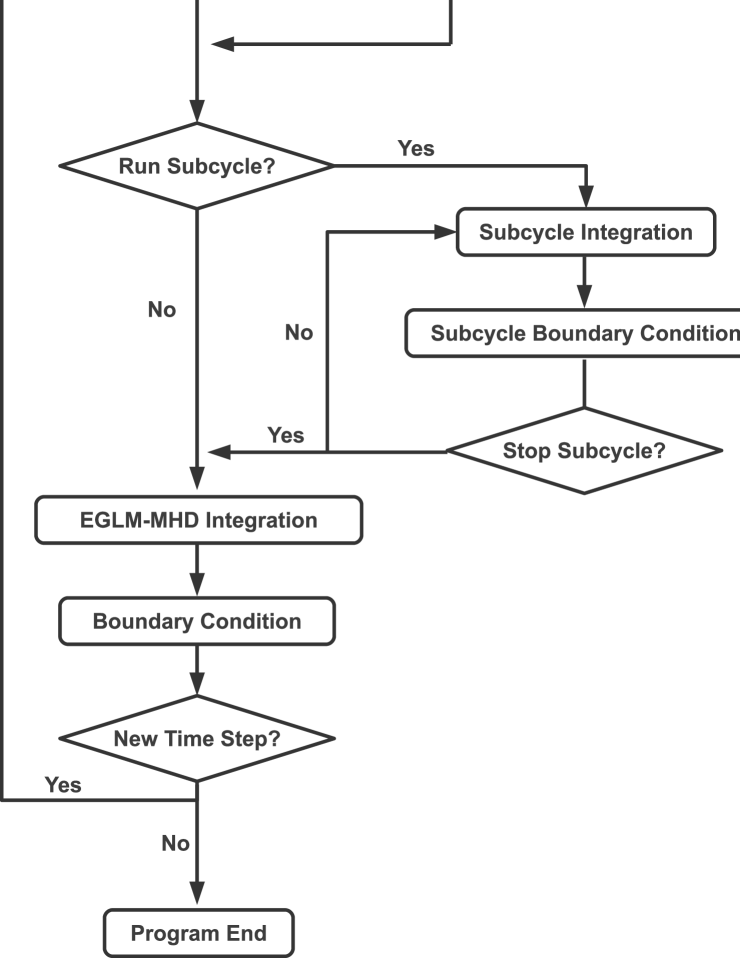
Figure 1: Schematic chart of our MAP code. The AMR algorithm includes the regriding, framework synchronization, load balance and neighbor statistics procedures. The time step in the subcycle is controlled by actual physical problem, e.g., the thermal conduction. The boundary condition of the subcycle is treated only for the specific physical quantity, i.e., the total energy. The boundary conditions contain the refluxing, data exchange and boundary fixing procedures.

$$\frac{\partial e}{\partial t}=\nabla\cdot\left(\kappa\nabla T\right)\,\,.$$ (40)

Assuming the grid is uniform, the one dimensional numerical scheme for this equation is given as

$$e_{i}^{n+1}=e_{i}+\frac{\Delta t}{{\Delta x}^{2}}\left(\sqrt{\kappa_{i}\kappa_{i+1}}\left(T_{i+1}-T_{i}\right)-\sqrt{\kappa_{i}\kappa_{i-1}}\left(T_{i}-T_{i-1}\right)\right)\,\,.$$ (41)

The time step used in the subcycle is given by

$$\Delta t=c_{cfl}\frac{\left(\min(\Delta x,\Delta y,\Delta z)\right)^{2}}{n_{dim}\max(\kappa T/p)}\,\,,$$ (42)

where $n_{dim}$ is the number of dimensions. The subcycle is simple and fast but one should be careful to deal with it. Since the other variables do not change with time during the subcycle, in our experience it is better to reduce the number of cycles to dozens or less to get the reliable results. Moreover, there should be a threshold for the temperature gradient in Eq. (40), because for any matter the speed of thermal conduction can not be infinite. That is a problem dependent parameter. So far, only the thermal conduction is calculated by the subcycle. If necessary, it is easy to add other physical process into the subcycle.

3.5 Resistivity

As for the resistivity terms $\mathbf{R}(R_{x},R_{y},R_{z})=-\nabla\times\left(\eta\nabla\times\mathbf{B}\right)$ and $R_{e}=-\nabla\cdot\left(\left(\eta\nabla\times\mathbf{B}\right)\times\mathbf{B}\right)$ in the induction equations (7) and (8), we use the simple central finite difference scheme to compute the current density first ($\mathbf{J}(J_{x},J_{y},J_{z})=\nabla\times\mathbf{B}$), and then the resistivity terms, i.e.:

$$(J_{x})_{i,j,k}=\frac{(B_{z})_{i,j+1,k}-(B_{z})_{i,j-1,k}}{2\Delta y}-\frac{(B_{y})_{i,j,k+1}-(B_{y})_{i,j,k-1}}{2\Delta z}\,\,\,$$

$$(J_{y})_{i,j,k}=\frac{(B_{x})_{i,j,k+1}-(B_{x})_{i,j,k-1}}{2\Delta z}-\frac{(B_{z})_{i+1,j,k}-(B_{z})_{i-1,j,k}}{2\Delta x}\,\,\,$$ (43)

$$(J_{z})_{i,j,k}=\frac{(B_{y})_{i+1,j,k}-(B_{y})_{i-1,j,k}}{2\Delta x}-\frac{(B_{x})_{i,j+1,k}-(B_{x})_{i,j-1,k}}{2\Delta y}\,\,,$$

$$(R_{x})_{i,j,k}=\frac{(\eta J_{y})_{i,j,k+1}-(\eta J_{y})_{i,j,k-1}}{2\Delta z}-\frac{(\eta J_{z})_{i,j+1,k}-(\eta J_{z})_{i,j-1,k}}{2\Delta y}\,\,\,$$

$$(R_{y})_{i,j,k}=\frac{(\eta J_{z})_{i+1,j,k}-(\eta J_{z})_{i-1,j,k}}{2\Delta x}-\frac{(\eta J_{x})_{i,j,k+1}-(\eta J_{x})_{i,j,k-1}}{2\Delta z}\,\,\,$$ (44)

$$(R_{z})_{i,j,k}=\frac{(\eta J_{x})_{i,j+1,k}-(\eta J_{x})_{i,j-1,k}}{2\Delta y}-\frac{(\eta J_{y})_{i+1,j,k}-(\eta J_{y})_{i-1,j,k}}{2\Delta x}\,\,,$$

$$R_{e}=\frac{\left(\eta(J_{z}B_{y}-J_{y}B_{z})\right)_{i+1,j,k}-\left(\eta(J_{z}B_{y}-J_{y}B_{z})\right)_{i-1,j,k}}{2\Delta x}\,\,\,$$

$$\frac{\left(\eta(J_{x}B_{z}-J_{z}B_{x})\right)_{i,j+1,k}-\left(\eta(J_{x}B_{z}-J_{z}B_{x})\right)_{i,j-1,k}}{2\Delta y}\,\,\,$$

$$\frac{\left(\eta(J_{y}B_{x}-J_{x}B_{y})\right)_{i,j,k+1}-\left(\eta(J_{y}B_{x}-J_{x}B_{y})\right)_{i,j,k-1}}{2\Delta z}\,\,,$$ (45)

where $R_{x}$, $R_{y}$ and $R_{z}$ are for the induction equation (7) and $R_{e}$ for the energy Eq. (8). The resistivity model can be modified to any form according to the user’s need.

3.6 Damping zone

The damping zone is a range where the MHD waves and matter motions can be damped to the initial condition. It is a kind of boundary condition because it is usually adjacent to the physical boundary. The goal of the zone is to stablize the boundary and to remove the non-physical inflows and outflows produced by the numerical error. Given a start position ($D_{s}$) and an end position ($D_{e}$) of the damping zone, the one dimensional damping function $D(x)$ is

$$D(x)=\frac{1}{2}\left(1-\tanh\left(\frac{6}{D_{e}-D_{s}}\left(x-\frac{D_{s}+D_{e}}{2}\right)\right)\right)$$ (46)

$$u(x)=u_{0}(x)(1-D(x))+u(x)D(x),$$ (47)

where $u_{0}$ is the initial value of the variable $u$. Fig. 2 shows the function of $D(x)$ with the situations $D_{s}>D_{e}$ and $D_{s}<D_{e}$, which correspond to the different damping directions, namely, physical waves and motions will vanish at the lower boundary for $D_{s}>D_{e}$ and at the higher boundary $D_{s}<D_{e}$. It is the same way to treat the damping zone in multiple dimensions. One can do it dimension by dimension or treat $x$, $y$ and $z$ directions together. The damping function only has effect on the density ($\rho$), velocities ($v_{x},v_{y},v_{z}$) and pressure ($p$), but not to the magnetic field. Because the modification of magnetic field will change the magnetic topological configuration which may destroy the divergence free condition leading to some non-physical results. It is noted that the damping zone can also produce some weak reflected waves. That is inevitable for most of the boundary conditions and these reflected waves have little effect on the results in our tests.

Figure 2: Damping function $D(x)$. Left panel shows the situation of $D_{s}>D_{e}$ where the left bounday is damped, while right panel shows the case with $D_{s}<D_{e}$ where the right bounday is damped.

3.7 Multiple spatial dimensions

All we discussed above is in 1D space. It is easy to extend the schemes to two or three dimensions. However, the method in extending the numerical scheme to multiple dimensions depends on the schemes. We treat the WENO scheme dimension by dimension in 2D and 3D. For the 2D case, the numerical flux in $x$-direction is calculated first and then the flux in $y$-direction by using the same variables at the old time. After that, the variables are updated to the new time by taking the numerical flux in $x$- and $y$- directions simultaneously. If the TVD Runge-Kutta method is available, the variables need to be calculated twice to update all variables. For TVD-MMC and TVD-LF methods, the dimension by dimension method is not necessary, since we can do all directions together. The formulae for 2D or 3D are easy to derive following the procedure in Sections 3.1 and 3.2. The time step in multiple dimensional problems are shown as follows:

$$\Delta t=c_{cfl}\frac{\min(\Delta x,\Delta y,\Delta z)}{n_{dim}\alpha_{g}}\,\,,$$ (48)

the $n_{dim}$ is the number of the dimensions, i.e. $n_{dim}=1$ for 1D, $n_{dim}=2$ for 2D and $n_{dim}=3$ for 3D and $\alpha_{g}$ is the global maximal wave speed. In Section 5, we show several 2D and 3D tests in some special test problems.

4 AMR parallelization strategy

The schematic chart (Fig. 1) shows the main process in the MAP code. The AMR parallelization is more difficult than the usual Eulerian meshes. The main difficults are: (1) how to arrange the structure for AMR hierarchical blocks? (2) how to guarantee the load balance when new blocks are generated? (3) how to apply the boundary conditions between different processors and between different refinement levels? We use the two dimensional MAP code to explain what we did in the AMR algorithm for simplicity and intuition. The aim of this section is to give a detailed explanation of the MAP code. Another purpose is to let the readers who have no idea about the AMR to know what is AMR and how to write an AMR code by themselves. MAP code implements the MPI parallelization which supports the MPICH2 and OpenMPI softwave, which are full MPI-2 standards. The other parallelization softwares like OpenMP which requires a shared-memory computer are not supported in our code.

4.1 Hierarchical structure

Supposing that we have a 2D computational domain with the total mesh cells of $8\times 8$, the domain initially is divided into 4 subdomains, labeled by 1, 2, 3, 4. Every block has the same cells $4\times 4$ and are surrounded by physical boundaries in gray and inner boundaries in yellow as shown in the upper left panel of Fig. 3 (note that the inner boundaries exist only between blocks). The numerical scheme discussed in Section 3 will solve the four blocks in turn. Then we can get the solution at the new time by gathering the data from all blocks.

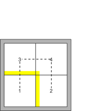
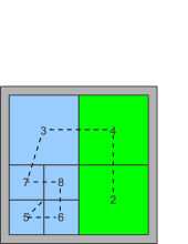
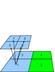
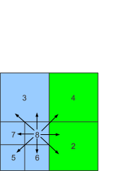
Figure 3: The AMR hierarchical structure. Upper left panel: The computational domain has four blocks with cells $4\times 4$ and the regions in gray and yellow are physical and inner boundaries. Only the inner boundaries of block 1 have been plotted in this panel. Note that the inner boundaries only exist between blocks. Upper middle panel: Blocks treated in processor 0 are in blue and those in processor 1 are in green. Block 1 has been refined to blocks 5, 6, 7 and 8. The inner boundaries have been omitted in this panel. Upper right panel: Another viewing angle for the middle panel without the physical and inner boundaries. The dashed lines in three panels are the H-curves. Lower left panel: the $child$ points of block 1 point to blocks 5, 6, 7 and 8. Lower middle panel: the $parent$ pointers of blocks 5, 6, 7 and 8 point to block 1. Lower right panel: The eight $neigh$ pointers of block 8 point to blocks 5, 6, 2, 2, 4, 3, 3 and 7, respectively.

Assuming that blocks 1 and 3 are in processor 0, blocks 2 and 4 in processor 1 and block 1 has already been refined as shown by the upper middle and upper right panels of Fig. 3. The number of cells in blocks 5, 6, 7, 8 is the same as the block 1, i.e. $4\times 4$, which means that the amount of calculation of the blocks 5, 6, 7, 8 is the same as the blocks 1, 2, 3, 4. All blocks are connected by the so-called link list. Every process includes two kind of link lists, one for collecting information in the local processor and the other one for global information, i.e. (1) global link list and (2) local link list. The local one refers to the links in the local processor while the global one links all blocks which exist in all processors as shown in Fig. 4. That is, the local ones are totally different in individual processors but the global ones are exactly the same. Actually, the global link is enough to complete the AMR algorithm, because one can judge which block in the link is located in the local processor. However, as we know, the global link sometimes is very long and may include several hundred thousand blocks, so the frequently used searching operations may take a long time. The order of these two links are arranged by the Hilbert space filling curve (H-curve) which is shown by the dashed lines in the upper panels of Fig. 3. The H-curve maps multidimensional data to one dimension while preserving locality of the data points. The order of the H-curve in the finer level blocks is determined by the parameters ($s\_pos$, $e\_pos$, $s\_point$ in Table 1) of the H-curve in their parent blocks.

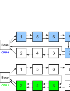
Figure 4: The global links (dashed arrows) and local links (solid arrows) between different blocks and different processors.

Every block, which is a STRUCTURE type variable in FORTRAN language, includes some information and data. The contents of information are listed in Table 1. Some examples: the $lv$ of block 8 is 2 and the $processor\_id$ of it is 0. The $id$ of block 8 is $\{\{1,1\},\{2,2\}\}$ and block 5 is $\{\{1,1\},\{1,1\}\}$. The $child$ pointers of block 1 point to blocks 5, 6, 7 and 8 (lower left panel of Fig. 3), respectively. The $parent$ pointers of blocks 5, 6, 7, 8 point to block 1 (lower middle panel of Fig. 3). The eight $neigh$ pointers of block 8 point to blocks 5, 6, 2, 2, 4, 3, 3, 7 (lower right panel of Fig. 3), respectively. The $neigh$ pointers have some identical values because, for instance, the right and lower right neighbors are the same.

Table 1: The block information.

Variable	Interpretation
$lv$	Level of current block.
$processor\_id$	Processor rank the current block belong to.
$nx,ny,nz$	Grid points or cells in $x$, $y$, $z$-direction of the current block.
$x,y,z$	$x$, $y$, $z$-coordinates of the current block.
$h\_number$	Position of the current block in the Hilbert curve.
$s\_pos,e\_pos,s\_point$	Used to generate the Hilbert curve in the finer level (array).
$id$	Position of the current block in the total AMR hierarchical levels (array).
$parent$	Link to the parent block of the current block (pointer).
$child$	Link to the children blocks of the current block, if no point to NULL (pointer array).
$neigh$	Link to the neighbor blocks of the current block, if no point to NULL (pointer array).
$next$	Link to the next block in the local link list (pointer).
$framework\_next$	Link to the next block in the global link list (pointer).

4.2 Load balance

Before introducing what is the load balance, we first introduce the definition of $framework$, which is very important to find a simple way to do the load balance. Just as its name implies, $framework$ is the framework of the AMR hierarchical structure. It is the global link list plus the all blocks’ information listed by Table 1. Like the global link list, the $framework$ in all processors should be exactly the same. In this case, block 8 in the processor 0 knows which is its right neighbor block located in the processor 1 as shown in Fig. 3. The processors have the same $framework$s, but they need not store all the variables of the blocks which belong to other processors. That is to say the blocks which belong to other processor have only the information listed by Table 1. In Fig. 4, the blocks in blue and green colors denote that only these blocks have allocated the memory for variables. It is noted that the blocks without the variable data can still be refined or destroyed. The $child$ blocks also have no variable data. And the memory required to store the entire global link list is very small.

The $framework$ structure has some advantages: (1) load balance can be done all at once rather than iteratively. That is to say, all blocks can be refined or destroyed to a suitable level according to the regrid algorithm. However, there is a special situation we have to carry on the regriding and load balance level by level (iteratively). When only a very small region has to refine to a very high level, while this region locates in only one processor, then the code has to allocate a huge number of memory in one processor. If the memory in one node is not enough, then the code crashes. Therefore, in our MAP code we can choose whether carrying on the regrid and load balance processes iteratively or not. (2) The data exchanging is simple. When carrying on the load balance, for instance, Processor 1 has to send the data of block A to processor 2, the processor 1 only needs to send the data of variables to the processor 2. And the block A (it already exists in processor 2 but without variable data) in processor 2 will be filled by this data. It needs not to send the neighbors information to processor 2 simultaneously. Because of the so-called $framework$, processors know the number of blocks in different processors and the total number of blocks in all processors. Thus, the code can calculate the load in different processors and balance the load by sending the block data from one processor to other one. The load is measured by the number of blocks which will be solved using the schemes described in Section 3. For instance, the block 3 in the upper middle panel of Fig. 3 will to sent to processor 1 by MPI calls because there are five blocks needed to be calculated in the processor 0 (the block 1 can be updated by the average values of its child blocks) and two blocks in the processor 1. This is not a rigorous balance because of the number of blocks which will be solved, the parent blocks (e.g. the block 1) which will be updated, and the boundary data which will be exchanged are different. However, this difference is very small when the total number of blocks is much greater than the number of processors.

After the load balance is done, the code has to do another important job: neighbor statistics. This is a preparation for the boundary conditions between different processors in the next several or dozens of time steps as shown in the schematic chart (Fig. 1). In this procedure, the code will record the number and the $id$ of blocks which need to reflux, the blocks which need to send data from fine blocks to coarse blocks, and the blocks which need to send data to the blocks at the same level. Once the number of the blocks is known, the code can allocate enough memory to store the data which will be sent or received in advance. When the block $id$ is known, the block will be found immediately and store its data to the allocated array or update its data from the allocated array. This can reduce the operations of allocating and freeing memory, so that the performance of the code can be greatly improved.

4.3 Boundary condition

The neighbor statistics can provide enough information for processing the boundary conditions quickly. As we described above, for boundary conditions we need to do: (1) data updating from the child blocks to the parent blocks; (2) reflux; (3) data exchange between blocks in the same level; (4) data exchange between different levels. We have several steps to do these. Every step has two small sub-steps: inter-processor first and then intra-processor. The inter-processor means the boundary conditions between different processors and the intra-processor stands for the boundary conditions inside one processor. The procedure is: (1) to update the parent data. In this step, we should care about shareblocks in the inter-processor case. The shareblock was firstly introduced by [11], which refers to the child blocks of one block located in different processors. Suppose that block 8 in Fig. 3 belongs to the processor 1 while its parent block belongs to the processor 0, so the block 8 is called the shareblock. The shareblock has to send all of its data (without the ghost region) to the corresponding position in the global link list of processor 0 in order to update the data of block 1; (2) to reflux the data between the fine-coarse boundaries as shown by the upper right panel of Fig. 3. Because the data of the coarse block 1 is updated by the fine blocks 5, 6, 7, 8 and the flux between the blocks 1 and 2 is changed, the block 2 has to use the new numerical flux to update its boundary data as suggested by [1] and [2]; (3) to exchange the $x$-direction data in the same level; (4) to exchange the $y$-direction data in the same level; (5) to exchange the $z$-direction data in the same level. The MAP code does not need extra requirement of MPI calls for the corner data (as shown by Fig. 5). The steps (3) - (5) can be explained by the left panel of Fig. 5. In this figure, the blue dashed ghost region will be updated by the data of the blue dashed box in the block 2; Then, the ghost region of the block 3 will be updated by the data of the red dashed box (already included the corner data) in the block 1. Of course, the steps (3) - (5) also treat the physical boundary conditions at the same time; (6) to update the ghost region of the fine block by interpolating the data of the coarse block at the fine-coarse boundaries. The only important thing here is that we should use a conservative interpolation. The formula is taken from [9]:

Figure 5: Left panel shows the data exchange at the same level. In the panel, we exchange the data in the $x$-direction first and then the $y$-direction. The corner data are also updated. The right panel shows a special situation in which the corner data can not be updated correctly.

$$u^{f}_{i,j,k}=u^{c}_{i^{c},j^{c},k^{c}}+\mathrm{minmod}\left(u^{c}_{i^{c}+1,j^{c},k^{c}}-u^{c}_{i^{c},j^{c},k^{c}},u^{c}_{i^{c},j^{c},k^{c}}-u^{c}_{i^{c}-1,j^{c},k^{c}}\right)\frac{x^{f}(i)-x^{c}(i^{c})}{\Delta x^{c}}\,\,\,$$

$$+\mathrm{minmod}\left(u^{c}_{i^{c},j^{c}+1,k^{c}}-u^{c}_{i^{c},j^{c},k^{c}},u^{c}_{i^{c},j^{c},k^{c}}-u^{c}_{i^{c},j^{c}-1,k^{c}}\right)\frac{y^{f}(j)-z^{c}(j^{c})}{\Delta y^{c}}\,\,\,$$ (49)

$$+\mathrm{minmod}\left(u^{c}_{i^{c},j^{c},k^{c}+1}-u^{c}_{i^{c},j^{c},k^{c}},u^{c}_{i^{c},j^{c},k^{c}}-u^{c}_{i^{c},j^{c},k^{c}-1}\right)\frac{z^{f}(k)-z^{c}(k^{c})}{\Delta z^{c}}\,,$$

where the fine block ($f$) is a child of the coarse block ($c$), the grids index ($i^{c},j^{c},k^{c}$) is for the coarse block and the coordinate ($x,y,z$) is defined at the center of the cell. The function of $\mathrm{minmod}$ is given by Eq. (32); (7) to fix the corner data. The steps (1) - (6) are successful to exchange almost all boundary data except one special situation shown by the right panel of Fig. 5. Only the lower left neighbor of the special block ($S$) is a coarse block. Before the fine-coarse step (6), the non-updated corner data of the normal block ($N$) are sent to the block ($S$) since the steps (3) - (5) is the advance step (6). Thus the corner data of the special block ($S$) need a fix step. In the MAP code, we just look for these so-called $S$ blocks and do the steps (4) - (5) again.

4.4 Framework synchronization

As we mentioned above, every processor knows the total information of the AMR hierarchical structure, it is possible to accomplish the load balance and the boundary conditions quickly and effectively. However, the next question is how to keep the $framework$ systems synchronous for every processor.

The framework synchronization is something like the cloning technique. The processors can generate the same $framework$ by the same $gene$. The local sequence of $gene$ is built by recording the $id$ of every block which will be regrided (including refining and destroying procedures) in a regridding operation in the current processor. The global sequence of $gene$ is obtained by merging all the local sequences. The MPI communication of $mpi\_allgatherv$ is necessary for such a merging. The criterion for refining or destroying will be discussed in Section 4.5. With the assumption that we have the same $framework$ in the current state, we can get the same $gene$ after regriding and then the code should generate the exactly same $framework$ at the next time step.

4.5 Regrid

The error estimation formula is taken from Matsumoto [9], Ziegler [11], which is determined by the first and second derivatives in the current level:

$$\left(\frac{B||\Delta u||_{2}}{|u|+\epsilon}+\frac{(1-B)||\Delta^{2}u||_{2}}{||\Delta u||_{2}+F\cdot\left(|u|+\epsilon\right)}\right)R^{\xi(L-1)}\,\,,$$ (50)

$$||\Delta u||_{2}=\frac{\sqrt{3}}{2}\left(\left(u_{i+1,j,k}-u_{i-1,j,k}\right)^{2}+\left(u_{i,j+1,k}-u_{i,j-1,k}\right)^{2}+\left(u_{i,j,k+1}-u_{i,j,k-1}\right)^{2}\right)^{1/2}\,\,,$$ (51)

$$||\Delta^{2}u||_{2}=(\left(u_{i+1,j,k}-2u_{i,j,k}+u_{i-1,j,k}\right)^{2}+\,\,\,$$

$$\left(u_{i,j+1,k}-2u_{i,j,k}+u_{i,j-1,k}\right)^{2}+\,\,\,$$ (52)

$$\left(u_{i,j,k+1}-2u_{i,j,k}+u_{i,j,k-1}\right)^{2})^{1/2}\,\,,$$

where the value of the filter $F$ is 0.05, $R$ is the refinement ratio and $L$ the level of the current block, and $\epsilon$ is taken as $10^{-12}$ for $\rho,p,T$ and $0.1$ for $\mathbf{v},\mathbf{B}$. The parameter $B=0.6$ specifies a bias toward the first derivatives for the criterion. The value $\xi$ makes the threshold for higher levels higher ($\xi<0$) or lower ($\xi>0$). When the error exceeds the given threshold values, the current block will be refined. If the errors estimated in every cell in the current block are larger than the threshold values, the child block of the current block can be destroyed. We also try to use the Richardson error estimation, however, this method usually takes a long time and is not so effective. For this reason, the Richardson error estimation is not included in the MAP code.

After several time steps the regridding operation will be carried on. The estimation interval for the next regridding is

$$\Delta t_{r}=c_{r}\frac{2n_{g}\min(\Delta x,\Delta y,\Delta z)}{\alpha_{g}}=c_{r}\frac{2n_{g}n_{dim}\Delta t}{c_{cfl}},$$ (53)

where $\Delta t_{r}$ is the time interval for the next regridding and $\Delta t$ is the time step of the simulation, which is taken from the finest level, and $\alpha_{g}$ is the global maximum wave speed. The different time steps for different levels will be achieved in the future work. Since the code checks the errors for every cell covering the ghost region so the length of buffer region in which the waves or discontinuities do not propagate to the coarse block before the next regridding time is $2n_{g}$ (Fig. 6), where $n_{g}$ is the number of ghost cells.

Figure 6: The blocks with blue borders show the coarse blocks and the red ones show the fine blocks. Assuming that the ghost cell is $1$, the buffer zone for the next regridding is the shadowy cells in the fine blocks since the MAP code checks every cell in the current block.

5 Numerical tests

Our MAP code is examined with a variety of test and application problems in this section. The 1D problems test the difference between different schemes and the accuracy of them. The 2D and 3D problems check the AMR parallel performance of our code. In all our test cases, we use the primitive variables to describe the initial conditions.

5.1 1D accuracy test

We test the accuracy of the three schemes, namely, MMC, LF and WENO by simplest advection problem: $(\rho,v_{x},v_{y},v_{x},B_{x},B_{y},B_{z},p)=((\sin(2\pi x)+2)/3,1,0,0,0,0,0,1)$ in the domain $[-0.5,0.5]$ with the periodic boundary. Lax-Friedrichs splitting for MMC and Lax-Friedrichs flux for LF and WENO are used in this test. The adiabatic index is $\gamma=1.4$. The $L^{1}$, $L^{2}$ and $L^{\infty}$ errors are listed in Table 2, which are defined as:

$$L^{1}(u)=\frac{1}{N}\sum_{i=1}^{N}|u_{i}^{n}-U_{i}|\,\,,$$ (54)

$$L^{2}(u)=\left(\frac{1}{N}\sum_{i=1}^{N}|u_{i}^{n}-U_{i}|^{2}\right)^{1/2}\,\,,$$ (55)

$$L^{\infty}(u)=\max_{1\leq i\leq N}(u_{i}^{n}-U_{i})\,\,,$$ (56)

where $U$ is the exact solution and $N$ the grid number. From Table 2, it can be seen that these schemes are second order accuracy and WENO scheme is better than the other two. This is why we mainly use WENO for most of our 2D and 3D tests.

Table 2: $L^{1}$, $L^{2}$ and $L^{\infty}$ error and order in 1D accuracy test.

Scheme	$N$	$L^{1}$ error	$L^{1}$ order	$L^{2}$ error	$L^{2}$ order	$L^{\infty}$ error	$L^{\infty}$ order
	$128$	$5.47\times 10^{-3}$	$-$	$7.27\times 10^{-3}$	$-$	$1.74\times 10^{-2}$	$-$
	$256$	$1.55\times 10^{-3}$	$1.82$	$2.34\times 10^{-3}$	$1.64$	$7.18\times 10^{-3}$	$1.27$
MMC	$384$	$7.37\times 10^{-4}$	$1.84$	$1.20\times 10^{-3}$	$1.65$	$4.25\times 10^{-3}$	$1.30$
	$512$	$4.32\times 10^{-4}$	$1.85$	$7.42\times 10^{-4}$	$1.66$	$2.91\times 10^{-3}$	$1.31$
	$640$	$2.84\times 10^{-4}$	$1.88$	$5.12\times 10^{-4}$	$1.66$	$2.17\times 10^{-3}$	$1.31$
	$128$	$4.64\times 10^{-3}$	$-$	$6.32\times 10^{-3}$	$-$	$1.72\times 10^{-2}$	$-$
	$256$	$1.31\times 10^{-3}$	$1.82$	$2.03\times 10^{-3}$	$1.64$	$7.12\times 10^{-3}$	$1.27$
LF	$384$	$6.20\times 10^{-4}$	$1.85$	$1.04\times 10^{-3}$	$1.65$	$4.22\times 10^{-3}$	$1.29$
	$512$	$3.62\times 10^{-4}$	$1.87$	$6.44\times 10^{-4}$	$1.66$	$2.90\times 10^{-3}$	$1.30$
	$640$	$2.38\times 10^{-4}$	$1.89$	$4.45\times 10^{-4}$	$1.66$	$2.17\times 10^{-3}$	$1.31$
	$128$	$2.99\times 10^{-3}$	$-$	$4.62\times 10^{-3}$	$-$	$1.24\times 10^{-2}$	$-$
	$256$	$7.04\times 10^{-4}$	$2.09$	$1.35\times 10^{-3}$	$1.77$	$4.68\times 10^{-3}$	$1.41$
WENO	$384$	$2.96\times 10^{-4}$	$2.14$	$6.54\times 10^{-4}$	$1.79$	$2.61\times 10^{-3}$	$1.44$
	$512$	$1.59\times 10^{-4}$	$2.16$	$3.89\times 10^{-4}$	$1.81$	$1.73\times 10^{-3}$	$1.44$
	$640$	$9.79\times 10^{-5}$	$2.17$	$2.60\times 10^{-4}$	$1.81$	$1.25\times 10^{-3}$	$1.46$

5.2 1D Brio-Wu shocktube test

This test is taken from [30], which is a standard 1.5D (one dimensional multi components) MHD shocktube problem. The initial conditions of the left ($x<0$) and right ($x>0$) states are $(\rho,v_{x},v_{y},v_{x},B_{x},B_{y},B_{z},p)_{L}=(1,0,0,0,0.75,1,0,1)$ and $(\rho,v_{x},v_{y},v_{x},B_{x},B_{y},B_{z},p)_{R}=(0.125,0,0,0,0.75,-1,0,0.1)$ with the adiabatic index $\gamma=2$. The length of computational domain is 1 and $x\in[-0.5,0.5]$. The upper panels of Fig. 7 show the comparison between the three kinds of schemes without the approximate Riemann solvers (Lax-Friedrichs splitting for MMC and Lax-Friedrichs flux for LF and WENO) while the lower panels show the same scheme (WENO) but with different Riemann solvers. From this figure, we found that the WENO and LF schemes are much better than the MMC scheme (upper panels). Although the MMC scheme has the same accuracy as the LF scheme, the former is not suitable to treat the MHD problem. HLLD and Roe Riemann solvers are more accurate than HLLC (lower panels). However, in our multi-dimensional tests, the HLLD and Roe solvers fail sometimes, thus we mainly use HLLC for our 2D and 3D test problems.

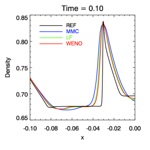
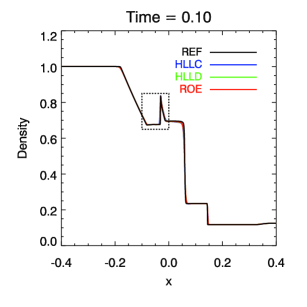
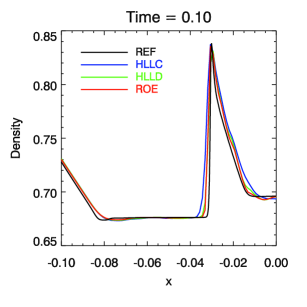
Figure 7: Comparsion between the modified Mac Cormack Scheme (MMC), Lax-Fridrichs scheme (LF), and weighted essentially non-oscillatory (WENO) scheme in the 1.5D MHD shocktube problem. The figure shows the range from $-0.4$ to $0.4$ at time $0.10$. The solid line is a reference solution with $4000$ cells, while the MMC, LF, WENO schemes are computed with $800$ cells. The lower panels are calculated based on the WENO scheme with different approximate Riemann solvers, i.e. HLLC, HLLD and Roe solver. The right panel is a zoom-in view of the dashed box in the left panel.

5.3 2D accuracy test

As the 1D advection test, we also test the convergence of the three schemes in 2D advection problem: $(\rho,v_{x},v_{y},v_{x},B_{x},B_{y},B_{z},p)=((\sin(2\pi(x+y/\sqrt{3})+pi/2)+2)/3,1,\sqrt{3},0,0,0,0,1)$ in the domain $[-0.5,0.5]\times[-\sqrt{3}/2,\sqrt{3}/2]$ with the periodic boundary. The velocity has angle of $\pi/6$ with the $y$-axis. Lax-Friedrichs splitting for MMC and Lax-Friedrichs flux for LF and WENO are used in this test. The adiabatic index $\gamma=1.4$. The $L^{1}$, $L^{2}$ and $L^{\infty}$ errors are listed in Table 3. As shown by this table, we got almost the same results with the 1D test. Moreover, we found that the extended 3D advection test also given the similar result, which is no longer necessary to discuss in this paper.

Table 3: $L^{1}$, $L^{2}$ and $L^{\infty}$ error and order in 2D accuracy test.

Scheme	$N$	$L^{1}$ error	$L^{1}$ order	$L^{2}$ error	$L^{2}$ order	$L^{\infty}$ error	$L^{\infty}$ order
	$64$	$1.89\times 10^{-2}$	$-$	$2.30\times 10^{-2}$	$-$	$4.82\times 10^{-2}$	$-$
	$128$	$6.35\times 10^{-3}$	$1.59$	$8.34\times 10^{-3}$	$1.48$	$2.09\times 10^{-2}$	$1.22$
MMC	$192$	$2.95\times 10^{-3}$	$1.90$	$4.32\times 10^{-3}$	$1.63$	$1.26\times 10^{-2}$	$1.25$
	$256$	$1.76\times 10^{-3}$	$1.80$	$2.70\times 10^{-3}$	$1.65$	$8.75\times 10^{-3}$	$1.27$
	$320$	$1.16\times 10^{-3}$	$1.90$	$1.86\times 10^{-3}$	$1.67$	$6.58\times 10^{-3}$	$1.29$
	$64$	$2.07\times 10^{-2}$	$-$	$2.49\times 10^{-2}$	$-$	$5.16\times 10^{-2}$	$-$
	$128$	$6.99\times 10^{-3}$	$1.58$	$9.09\times 10^{-3}$	$1.47$	$2.25\times 10^{-2}$	$1.21$
LF	$192$	$3.35\times 10^{-3}$	$1.83$	$4.67\times 10^{-3}$	$1.65$	$1.35\times 10^{-2}$	$1.25$
	$256$	$1.96\times 10^{-3}$	$1.87$	$2.91\times 10^{-3}$	$1.64$	$9.38\times 10^{-3}$	$1.28$
	$320$	$1.29\times 10^{-3}$	$1.87$	$2.01\times 10^{-3}$	$1.66$	$7.04\times 10^{-3}$	$1.29$
	$64$	$1.78\times 10^{-2}$	$-$	$2.09\times 10^{-2}$	$-$	$4.14\times 10^{-2}$	$-$
	$128$	$4.39\times 10^{-3}$	$2.05$	$6.40\times 10^{-3}$	$1.72$	$1.63\times 10^{-2}$	$1.36$
WENO	$192$	$1.90\times 10^{-3}$	$2.07$	$3.15\times 10^{-3}$	$1.76$	$9.26\times 10^{-3}$	$1.40$
	$256$	$1.05\times 10^{-3}$	$2.08$	$1.89\times 10^{-3}$	$1.78$	$6.17\times 10^{-3}$	$1.42$
	$320$	$6.64\times 10^{-4}$	$2.06$	$1.27\times 10^{-3}$	$1.79$	$4.49\times 10^{-3}$	$1.43$

5.4 2D parallelization efficiency test

A simple MHD 2D test is a blast wave. The problem can generate several shocks from the central high gas pressure zone, it is very suitable to test the AMR algorithm and the parallel efficiency. The density ($\rho$) and magnetic field ($B_{x},B_{y},B_{z}$) are uniform in the domain $[-0.5,0.5]\times[-0.5,0.5]$ with the value $1$ and $(1/\sqrt{2},1/\sqrt{2},0)$, respectively. A small hot area is located at the center of the domain, i.e. $p=10$ within the circle $x^{2}+y^{2}\leq 0.1^{2}$, whereas $p=1$ out of this circle. Adiabatic index is $\gamma=5/3$. The left panel of Fig. 8 shows the pressure distribution at time $0.16$ and the right one shows the AMR mesh with the refinement level $L=5$. Since the base resolution is $256\times 256$, the effective resolution is $4096\times 4096$. Fig. 8 corresponds to a 8-processor run, the parallelization efficiency for other number of processors are listed in Table 4, where $N_{p}$ is the number of processors, $Blocks$ indicates the total number of blocks in all processors at time 0.16. The efficiencies higher than 1 may due to the speed fluctuation of the supercomputer.

Table 4: Parallelization efficiency for Blast wave test (AMR level $L=5$).

$N_{p}$	Blocks	Time	Efficiency
$1$	$15512$	$88504$ s	$1$
$2$	$15512$	$43595$ s	$1.02$
$4$	$15512$	$21941$ s	$1.01$
$8$	$15512$	$11327$ s	$0.98$
$16$	$15512$	$5731$ s	$0.97$
$32$	$15512$	$2908$ s	$0.95$
$64$	$15504$	$1521$ s	$0.90$
$128$	$15504$	$831$ s	$0.83$

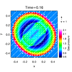
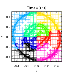
Figure 8: Left panel is the gas pressure distribution with the velocity arrows and magnetic field lines at time 0.16. The right panel shows the AMR mesh with the refinement level 5. The eight colors in the right panel stand for the blocks occupied by the eight processors.

5.5 2D divergence free test

The test was introduced by [33] to check the conservation of the divergence-free condition. If we had not taken this condition into account, the code may give us non-physical results in some MHD applications. The problem domain is $[-0.5,0.5]\times[-0.5,0.5]$, with the uniform density ($\rho=1$) and velocity ($v_{x}=1$, $v_{y}=1$, $v_{z}=0$). The magnetic configuration is given by $B_{x}=-B_{0}y/r$, $B_{y}=B_{0}x/r$ and $B_{z}=0$ in the region $r=\sqrt{x^{2}+y^{2}}<0.2$. In this region, we set $p=1-B_{0}^{2}/2$ for magnetostatic equilibrium and $p=1$ for outside of this region. Adiabatic index $\gamma=5/3$ and $B_{0}=1\times 10^{-3}$. The results are displayed in Fig. 9. The magnetic loops advect across the boundary twice when the dimensionless time is $2$. As shown in Fig. 9, the magnetic loops without divergence cleanance are distorted (middle panel). However, when the divergence cleanance is conducted, the loops keep their original shapes (right panel). The $\nabla\cdot\mathbf{B}$ errors are plotted with the function of time in the Fig. 10. In this figure, we show the performances of the three schemes. As expected, the methods using EGLM-MHD equations can maintain the error one order of magnitude smaller than the methods using pure MHD. The method with higher resolution also given less $\nabla\cdot\mathbf{B}$ error. Although it is not so perfect as the CT schemes, EGLM-MHD has its advantages: (1) it is easy to be equipped in the existed MHD codes; (2) it can damp the non-divergence error produced by the rapidly-changing boundaries.

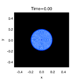
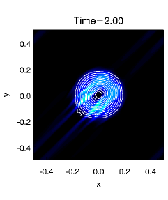
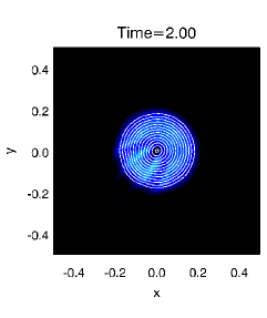
Figure 9: Total magnetic pressure distributions with the magnetic field lines of divergence free test. Left panel: The initial condition; Middle panel: advection result at time $2$ without divergence cleanance method; Right panel: advection result at time $2$ using EGLM-MHD with a coefficient $c_{d}=0.18$ as described in Section 2. This simulation is carried on by using the WENO scheme with the Lax-Friedrichs flux. The resolution in this test is $256\times 256$, no AMR involved.

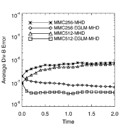
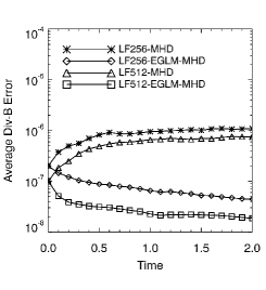
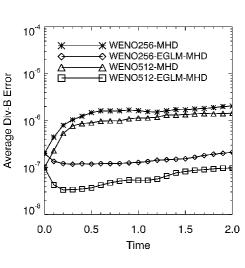
Figure 10: The $\nabla\cdot\mathbf{B}$ average errors with a function of time for different methods and resolutions (the numbers 256 and 512 mean the resolutions of $256\times 256$ and $512\times 512$). Left panel: the MMC scheme; Middle panel: LF scheme; Right panel: WENO scheme. Lax-Friedrichs splitting for MMC and Lax-Friedrichs flux for LF and WENO are used in this test.

5.6 2D magnetic rotor

This test suite is introduced by Balsara and Daniel [42], which is used to test the propagation of strong torsional Alfvén waves. The rotating disk in the computational center generates shocks and waves from the strong shearing surface between the rotating disk and the static ambient fluid. We use the initial conditions as described by Tóth [38] which involves a higher initial velocities. It is better to test the robustness of our code. The computational domain is $[-0.5,0.5]\times[-0.5,0.5]$, the initial distributions are:

$$\rho=\left\{\begin{array}[]{ll}10&\ \ \textrm{for}\ \ r<r_{0}\\ 1+9f&\ \ \textrm{for}\ \ r_{0}\leq r\leq r_{1}\\ 1&\ \ \textrm{for}\ \ r>r_{1}\\ \end{array}\,\,,\right.$$ (57)

$$v_{x}=\left\{\begin{array}[]{ll}-2y/r_{0}&\ \ \textrm{for}\ \ r<r_{0}\\ -2fy/r&\ \ \textrm{for}\ \ r_{0}\leq r\leq r_{1}\\ 0&\ \ \textrm{for}\ \ r>r_{1}\\ \end{array}\,\,,\right.$$ (58)

$$v_{y}=\left\{\begin{array}[]{ll}2x/r_{0}&\ \ \textrm{for}\ \ r<r_{0}\\ 2fx/r&\ \ \textrm{for}\ \ r_{0}\leq r\leq r_{1}\\ 0&\ \ \textrm{for}\ \ r>r_{1}\\ \end{array}\,\,,\right.$$ (59)

where, $r=\sqrt{x^{2}+y^{2}}$ and $f=(r_{1}-r)/(r_{1}-r_{0})$ with $r_{0}=0.1$ and $r_{1}=0.115$. $f$ function helps to reduce initial transients. The gas pressuse $p=1$ and magnetic field $B_{x}=5/\sqrt{4\pi},B_{y}=0$ are uniform. The third components of velocity and magnetic field are set to zero. Adiabatic index $\gamma=1.4$. The density, gas pressure, Mach number and magnetic pressure distributions at Time = 0.15 are shown in Fig. 11. The test is based on the WENO scheme with the resolution of $400\times 400$ and no approximate Riemann solvers included. From this figure we can observe that the torsional Alfvén waves are generated. The EGLM-MHD equations prevent the magnetic monopoles to form and the contours of Mach number keep the shape of concentric circles. Other methods (LF and MMC) show almost the same results.

Figure 11: The density, gas pressure, Mach number and magnetic pressure distributions at Time = 0.15. There are 30 equally spaced contours between the maximum and minimum for each plot. This test is based on the WENO scheme with the resolution of $400\times 400$ and the Lax-Friedrichs flux.

5.7 2D magnetic reconnection application

In this subsection we mainly test the effect of resistivity in the magnetic reconnection process. This kind of resistivity may due to some microscopic instabilities, although how these instabilities drive the macroscopic reconnection is still not clear. The velocities ($v_{x}$,$v_{y}$,$v_{z}$) are zero in the initial state. We set a uniform density ($\rho=1$) and pressure ($p=0.1$) distributions with an anti-parallel magnetic configuration (see below) in the computational domain ($[-0.5,0.5]\times[-2,2]$) as follows:

$$B_{x}=0\,\,,$$ (60)

$$B_{y}=\left\{\begin{array}[]{ll}-1&\ \ \textrm{for}\ \ x<-L_{r}\\ \sin(\pi x/2L_{r})&\ \ \textrm{for}\ \ |x|\leq L_{r}\\ 1&\ \ \textrm{for}\ \ x>L_{r}\\ \end{array}\,\,,\right.$$ (61)

$$B_{z}=\left\{\begin{array}[]{ll}0&\ \ \textrm{for}\ \ x<-L_{r}\\ \cos(\pi x/2L_{r})&\ \ \textrm{for}\ \ |x|\leq L_{r}\\ 0&\ \ \textrm{for}\ \ x>L_{r}\\ \end{array}\,\,,\right.$$ (62)

where $L_{r}=0.05$ is the half width of the resistivity region in the $x$-direction. The resistivity has the form $\eta=\eta_{0}\left(\cos(\pi x/0.1)+1\right)\left(\cos(\pi y/0.4)+1\right)/4$ in the small region $[-0.05,0.05]\times[-0.2,0.2]$. The reconnection becomes fast when localized resistivity is included. The simulation results are shown in Fig. 12. We get a fast magnetic reconnection results by a localized resistivity region [43, 44] at the center of the domain. The magnetic reconnection releases the magnetic energy to heat the matter located at the center of the computation box. The upward and downward outflows are accelerated to the Alfvén speed by the magnetic tension force. This test is based on the WENO scheme with the Lax-Friedrichs flux. The effective resolution is $2048\times 4096$ and we can observe some plasmoids formed at the positions $x=0$ and $y=\pm 0.2$.

In Fig. 13, we can see five variable distributions along the white horizontal line in the right panel of Fig. 12 and the reconnection rate as a function of time. The variable distributions clearly show the slow mode shock in the ranges ($-0.03<x<-0.01$ and $0.01<x<0.03$). The variables sharply changed between the upstream and the downstream of this shock. The reconnection rate is calculated by $V_{in}/V_{A}$, where $V_{in}$ is the inflow speed and $V_{A}$ the Alfvén speed. As shown by the lower right of Fig. 13, the reconnection rate reaches to the maximum around the time 1.0 and the value of this rate is about 0.76 which is in the range of $0.01-0.1$ as expected by Petschek [45].

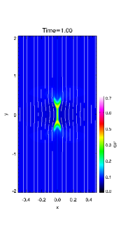
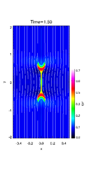
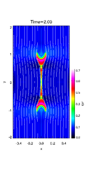
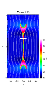
Figure 12: Gas pressure distributions with velocity arrows and magnetic field lines at time 1.0, 1.5, 2.0 and 2.5. This test is based on the WENO scheme with the Lax-Friedrichs flux. Base resolution is $128\times 256$ and the maximum refinement level is 5.

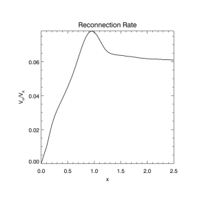
Figure 13: The distributions of gas pressure, magnetic pressure, x-component velocity, y-component velocity, density along the white line in Fig. 12 at time 2.5. The lower right panel is the magnetic reconnection rate as a function of the time. The dashed lines show the velocity value of 0.

5.8 2D thermal conduction test

In this test, we test the thermal condction effect with the method of subcycle and without the subcycle. Considering fully ionization plasma ($\gamma=5/3$), the thermal conduction can only transfer the energy along the magnetic field lines. The conduction term $\nabla\cdot\left(\kappa\nabla T\right)$ in the MHD energy equation (Eq. (8)) is changed to the form $\nabla\cdot\left(\kappa_{0}T^{5/2}(\mathbf{B}\cdot\nabla T)\mathbf{B}/B^{2}\right)$, where $\kappa_{0}$ is a coefficient for thermal conduction (we take $\kappa_{0}=0.001$ in this test). The initial condition is very simple. In the computational domain ($[-0.5,0.5]\times[-0.5,0.5]$), we have uniform distributions: $(\rho,v_{x},v_{y},v_{x},B_{x},B_{y},B_{z},p)=(0.1,0,0,0,1,1,0,0.1)$. Besides, we set a small hot range ($\rho(x,0)=0.01$ in the range $|x|<0.1$) at the bottom of the boundary and the heat will be transferred along the oblique magnetic field lines as shown by Fig. 14. The bottom boundary is maintained as its initial value in the total evolution, while the left and right boundaries are periodic. Finally, the top boundary is free.

Fig. 14 shows that the results with and without subcycle almost have the same results. Additional comparison is given in Fig. 15 which taken the temperature distributions along a vertical line ($x=0.4$) for both the upper right and the lower right panels. We can see that the shapes of two results are identical. We checked the values for both cases and found the difference between two case is less than $0.5\%$. However, the time spent in both cases are not in the same order of magnitude. For instance, in this test, the total elapsed time is 2225.27 seconds for the subcycle case while 28770.04 seconds for the case without subcycle. That is to say, we can get a almost identical result in a relatively short time by using the subcycle method.

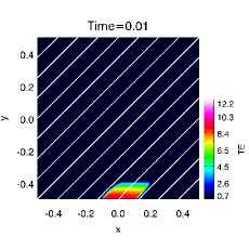
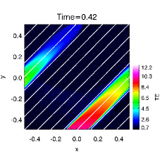
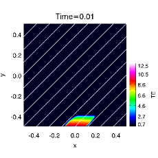
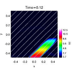
Figure 14: Temperature distributions with the magnetic field lines (white lines) at time 0.01, 0.12 and 0.42. The upper and lower panels show the results with subcycle and without subcycle, respectively. This test is based on the WENO scheme with the Lax-Friedrichs flux.

Figure 15: Comparison of temperature distributions for the test with and without subcycle. The distributions are along the line $x=0.4$ at the Time = 0.42 for both cases shown in Fig. 14.

5.9 3D Rayleigh Taylor instability application

In the last application we check the performance of our MAP code in the 3D domain $[-0.5,0.5]\times[-0.5,0.5]\times[-1,1]$ with a gravity field ($g_{x}=0$, $g_{y}=0$, $g_{z}=-1$). The heavy gas ($\rho=3$) fills the upper half of the computational box ($z>0$) while the light gas ($\rho=1$) fills the lower half ($z<0$). A velocity perturbation is introduced in the $z$-direction to trigger instability. The mathematical form of the perturbation is $v_{x}=0$, $v_{y}=0$, $v_{z}=0.01(1+\cos(\pi x))(1+\cos(\pi y))(1+\cos(\pi z))$ in the cubic region $[-0.5,0.5]\times[-0.5,0.5]\times[-0.5,0.5]$. The pressure ($p$) is changed from $1$ at the bottom boundary to $5$ at the top boundary to get the hydrostatic balance. There is no magnetic field and the adiabatic index $\gamma=7/5$. The resuls are shown in Fig. 16. The statistics of the time consumption is given in Table 5 for a 128-processor run and AMR level $L=4$.

This simulation can test the performance of the source term and the symmetry of our code. As we can observe from Fig. 16, the Rayleigh Taylor instability is successfully formed and the Kelvin-Helmholtz instability is also generated at the interface. The WENO scheme maintains a good symmetrical property in this problem. However, as we know, the final structure of this Rayleigh Taylor instability test is sensitive to the numerical diffusion of the scheme we used. If we use the Lax-Fridrichs flux instead of HLLC soler, the final shape of the interface between the light and heavy fluids will differ wildly from the result shown in Fig. 16. Thus, we do not give the results got by other methods.

Figure 16: Simulation result of the 3D rayleigh taylor instability at the time 3.0, 3.5 and 4.0. Left panels: density distribution displayed by the volume rendering, which is visualized by the tool $VisIt$ developed by the Department of Energy (DOE) Advanced Simulation and Computing Initiative (ASCI). Middle panels: the density distribution on the $x$-$z$ plane at the position $y=0$. Right panels: the density distribution on the $x$-$y$ plane at the position $z=0$. The test is based on the WENO scheme with the HLLC approximate Riemann solver.

Table 5: Statistics of the time consumption for the 3D rayleigh Taylor instability.

$N_{p}$	$128$
Levels	$4$
Effective resolution	$256\times 256\times 512$
Total elapsed time	5h 55m 11.15s
Regridding, Load Balance	0.46%
Integration	83.64%
Data output	0.05%
Boundary condition	8.590%
Other (initial condition, data check, calculate minimum $\Delta t$)	6.96%

6 Summary

We have presented an MHD code with adaptive mesh refinement and parallelization for astrophysics, named MAP. We use three kind of schemes, namely modified Mac Cormack Scheme (MMC), Lax-Fridrichs scheme (LF) and weighted essentially non-oscillatory (WENO) scheme, combined with TVD limiters and approximate Riemann solvers (HLLC, HLLD, and Roe solvers). The divergence free condition is guaranteed by the EGLM-MHD equations. As for the AMR parallelization strategy, the conception of $framework$ and $gene$ may be discussed with a different names in other codes. Nevertheless, there must be many differences from other existing codes, for instance, the treatments of the load balance, boundary condition, etc. It is also useful for the readers to understand what is AMR or how to develop an AMR code by themselves.

Our MAP code can be easily applied to the actual problems by simply modifying the modules of initial and boundary conditions. For some special cases, the resistivity model and the damping region can also be changed. We are already using our MAP code for some solar MHD applications, for example, magnetic reconnection between emerging flux and the background canopy-type magnetic configuration which is aimed to explain the microflares in the solar chromosphere and corona. These will be discussed in detail in future papers.

This paper only describes the first version of our MAP code. The code needs to be further improved in many aspects. Up to now, an improvement should be done in the next job is the radiative transfer. As well known, in the solar photosphere and chromosphere, the optically-thick radiation is very important for the energy transfer. How to implement it into MHD equations should be a heavy work and needs a long time to code and test. Optically-thin case is relatively easy to include, for instance, one can write a subroutine for adding a source term to include the optically-thin transfer. The other implements like the mesh geometries in cylindrical and spherical grids will be added in the next version. It is emphasized here again that we did not take the schemes with the accuracy higher than two orders into account as we mentioned in Section 1, since many operations in the AMR algorithm and the treatment in source terms, for instance, the radiation transfer mentioned above, can not reach such a higher accuracy. How to improve the accuracy globally is another topic which is out of the scope of this paper.

References

- Berger and Oliger [1984] M. J. Berger, J. Oliger, J. Comput. Phys. 53 (1984) 484.
- Berger and Colella [1989] M. J. Berger, P. Colella, J. Comput. Phys. 82 (1989) 64.
- DeZeeuw and Powell [1993] D. DeZeeuw, K. G. Powell, J. Comput. Phys. 104 (1993) 56.
- Morton [1966] G. M. Morton, Technical Report, Canada: IBM Ltd., Ottawa, 1966.
- Hilbert [1891] D. Hilbert, Math. Ann. 38 (1891) 459.
- Fryxell et al. [2000] B. Fryxell, K. Olson, P. Ricker, F. X. Timmes, M. Zingale, D. Q. Lamb, P. MacNeice, R. Rosner, J. W. Truran, H. Tufo, Astrophs. J. Suppl. 131 (2000) 273.
- Keppens et al. [2003] R. Keppens, M. Nool, G. Tóth, J. P. Goedbloed, Comput. Phys. Comm. 153 (2003) 317.
- Mignone et al. [2007] A. Mignone, G. Bodo, S. Massaglia, T. Matsakos, O. Tesileanu, C. Zanni, A. Ferrari, Astrophs. J. Suppl. 170 (2007) 228.
- Matsumoto [2007] T. Matsumoto, Publ. Astron. Soc. Japan 59 (2007) 905.
- Ziegler [2005] U. Ziegler, Comput. Phys. Comm. 170 (2005) 153.
- Ziegler [2008] U. Ziegler, Comput. Phys. Comm. 179 (2008) 227.
- Fromang et al. [2006] S. Fromang, P. Hennebelle, R. Teyssier, Astron. Astrophys. 457 (2006) 371.
- Balsara [2001] D. S. Balsara, J. Comput. Phys. 174 (2001) 614.
- van der Holst et al. [2011] B. van der Holst, G. Tóth, I. V. Sokolov, K. G. Powell, J. P. Holloway, E. S. Myra, Q. Stout, M. L. Adams, J. E. Morel, S. Karni, B. Fryxell, R. P. Drake, Astrophs. J. Suppl. 194 (2011) 23.
- Miniati and Martin [2011] F. Miniati, D. F. Martin, Astrophs. J. Suppl. 195 (2011) 5.
- Almgren et al. [2010] A. S. Almgren, V. E. Beckner, J. B. Bell, M. S. Day, L. H. Howell, C. C. Joggerst, M. J. Lijewski, A. Nonaka, M. Singer, M. Zingale, Astrophs. J. 715 (2010) 1221.
- Zhang et al. [2011] W. Zhang, L. Howell, A. Almgren, A. Burrows, J. Bell, Astrophs. J. Suppl. 196 (2011) 20.
- MacNeice et al. [2000] P. MacNeice, K. M. Olson, C. Mobarry, R. de Fainchtein, C. Packer, Comput. Phys. Comm. 126 (2000) 330.
- Cho [2011] CHOMBO library, Website, 2011. https://seesar.lbl.gov/anag/chombo/.
- Box [2011] BoxLib library, Website, 2011. https://ccse.lbl.gov/index.html.
- Dedner et al. [2002] A. Dedner, F. Kemm, D. Kroner, C.-D. Munz, T. Schnitzer, M. Wesenberg, J. Comput. Phys. 175 (2002) 645.
- Evans and Hawley [1988] C. R. Evans, J. F. Hawley, Astrophs. J. 332 (1988) 659.
- Yu and Liu [2000] H. Yu, Y.-P. Liu, J. Comput. Phys. 173 (2000) 1.
- Tóth and Odstrčil [1996] G. Tóth, D. Odstrčil, J. Comput. Phys. 128 (1996) 82.
- Jiang and Wu [1999] G.-S. Jiang, C.-C. Wu, J. Comput. Phys. 150 (1999) 561.
- Harten [1997] A. Harten, J. Comput. Phys. 135 (1997) 260.
- Gurski [2001] K. F. Gurski, SIAM J. Sci. Comput. 25 (2001) 2165.
- Miyoshi and Kusano [2005] T. Miyoshi, K. Kusano, J. Comput. Phys. 208 (2005) 315.
- Roe [1981] P. L. Roe, J. Comput. Phys. 43 (1981) 357.
- Brio and Wu [1988] M. Brio, C. C. Wu, J. Comput. Phys. 75 (1988) 400.
- Colella [1984] P. Colella, J. Comput. Phys. 54 (1984) 174.
- Dai and Woodward [1994] W. Dai, P. R. Woodward, J. Comput. Phys. 115 (1994) 485.
- Gardiner and Stone [2005] T. A. Gardiner, J. M. Stone, J. Comput. Phys. 205 (2005) 509.
- Gardiner and Stone [2008] T. A. Gardiner, J. M. Stone, J. Comput. Phys. 227 (2008) 4123.
- Jiang and Shu [1996] G.-S. Jiang, C.-W. Shu, J. Comput. Phys. 126 (1996) 202.
- Brackbill and Barnes [1980] J. U. Brackbill, D. C. Barnes, J. Comput. Phys. 3 (1980) 426.
- Powell et al. [1999] K. G. Powell, L. P. Roe, T. J. Linde, T. I. Gombosi, D. L. De zeeuw, J. Comput. Phys. 154 (1999) 284.
- Tóth [2000] G. Tóth, J. Comput. Phys. 161 (2000) 605.
- Chen et al. [1999] P. F. Chen, C. Fang, Y. H. Tang, M. D. Ding, Astrophs. J. 513 (1999) 516.
- Roe [1989] P. L. Roe, Lecture Notes in Physics 323 (1989) 69.
- Butcher [2005] J. Butcher, Numerical Methods for Ordinary Differential Equations, UK: John Wiley & Sons, Ltd, Chichester, 2005.
- Balsara and Daniel [1999] D.-S. Balsara, S.-S. Daniel, J. Comput. Phys. 149 (1999) 270.
- Jiang et al. [2010] R. L. Jiang, C. Fang, P. F. Chen, Astrophs. J. 710 (2010) 1387.
- Jiang et al. [2011] R. L. Jiang, K. Shibata, H. Isobe, C. Fang, Astrophs. J. Lett. 726 (2011) L16.
- Petschek [1964] H. E. Petschek, NASA Special Publication 50 (1964) 425.