Remarks concerning bulk viscosity of hadron matter in relaxation time ansatz

Abstract

The bulk viscosity is calculated for hadron matter produced in heavy-ion collisions, being described in the relaxation time approximation within the relativistic mean-field-based model with scaled hadron masses and couplings. We show how different approximations used in the literature affect the result. Numerical evaluations of the bulk viscosity with three considered models deviate not much from each other confirming earlier results.

1 Introduction

Recently, interest in the transport coefficient issue for hadronic and quark matter has essentially increased due to clarifying the role of viscosity in extraction of flow parameters from heavy-ion collisions, see review-article [1]. Viscosity coefficients in a weakly coupled scalar field theory at an arbitrary temperature can be evaluated directly from the first principles using expansion of the Kubo formulas in terms of ladder diagrams in the imaginary time formalism [2]. Unfortunately, similar analysis for more general cases is unavailable. Therefore, in order to evaluate transport coefficients in multi-component systems with a strong coupling between species, one often uses a kinetic approach. Thus, one can exploit the relaxation time approximation to the Boltzmann-like quasiparticle kinetic equations. The shear and bulk viscosities of the hadron and the quark-gluon plasma phases of strongly interacting matter at finite temperature and baryon density were evaluated, see Refs. [3, 4, 5]. In [6, 7, 8], a similar analysis was performed for purely gluon matter. Besides the use of the relaxation time approximation, one needs to do some extra assumptions in order to proceed further. In [7], we studied how different ansatze used in the literature affect the result for shear and bulk viscosities for gluon matter. We found that the result for the shear viscosity was robust with respect to different ansatz reductions, whereas the value of the bulk viscosity significantly depends on them. In this note we study how different approximations used in the literature affect the bulk viscosity of the hadron matter.

2 Model equations

As in [4], we describe the hadron phase in terms of the quasiparticle relativistic mean-field (RMF)-based model with the scaling hadron mass-couplings (SHMC) successfully applied earlier to the description of heavy-ion collision reactions  [9]. The model used is an extension of the model [10] applied there for the cold dense hadron matter. Bearing in mind its application to heavy-ion collisions, we deal with a RMF-based model of iso-symmetric non-equilibrium hadron matter with $\sigma$- and $\omega$-meson mean fields and in contrast with ordinary RMF models we assume that not only baryon but also other hadron masses might depend on the $\sigma$-meson mean field. Also excitations emerging from the $\sigma$ and $\omega_{0}$ mean fields are incorporated. We study the system with zero net strangeness and use the same hadron set, as in [9, 4]. Considering small deviations from local equilibrium we keep only first-order gradient terms. Further details can be found in the mentioned works [9, 4].

We start with the Lagrangian of SHMC model [9] from where expressions are reproduced for the baryon/strangeness 4-current and the energy-momentum tensor densities [4]:

$$J^{\mu}_{B,S} = \sum_{a}t_{a}^{B,S}\int\mathrm{d}\Gamma_{a}\frac{p^{\mu}_{a}}{E_{a}}\,f_{a}(x,\vec{p})~{},$$ (1)

$$T^{\mu\nu} = \sum_{a}\int\mathrm{d}\Gamma_{a}\frac{(p_{a}^{\mu}+X_{a}^{\mu})p^{\nu}_{a}}{E_{a}}\,f_{a}(x,\vec{p})+T^{\mu\nu}_{\rm MF}~{}.$$ (2)

Here ${\rm d}\Gamma_{a}=d_{a}\frac{{\rm d}^{3}p}{(2\pi)^{3}}~{},\quad p_{a}^{\mu}=\left(E_{a},\vec{p}\right)~{},$

$$E_{a}=\sqrt{\vec{p}^{\,2}+m_{a}^{*\,2}(\sigma)}~{},\quad X_{a}^{\mu}=X^{0}_{a}(\sigma,\omega_{0})\,\delta^{\mu 0}~{},$$ (3)

$t_{a}^{B},\ t_{a}^{S}$ are the baryon and strange charges of the $a$-hadron (antiparticles are included), $d_{a}$ is the degeneracy factor, $m_{a}^{*}(\sigma)$ is the effective mass, $f_{a}$ is the quasiparticle distribution function, $\sigma$ and $\omega_{0}$ are mean scalar and vector meson fields, $\omega^{\mu}=(\omega_{0},\vec{0})$, $X_{a}^{0}\sim\omega_{0}$,

$$T^{\mu\nu}_{\rm MF} = g^{\mu\nu}\left[U(\sigma)-V(\sigma,\omega)\right],$$ (4)

$$U(\sigma) = \frac{m_{\sigma}^{*\,2}(\sigma)\sigma^{2}}{2}+U_{\rm NL}(\sigma),$$

$$V(\sigma,\omega) = \frac{m_{\omega}^{*\,2}(\sigma)\omega_{0}^{2}}{2},$$

where $U_{\rm NL}(\sigma)$ is the non-linear potential of the $\sigma$ field. In general, since we derive (2) from the Lagrangian, in our mean-field approach the energy-momentum tensor can be symmetrized following the standard rule, e.g. see [11]. In this note we study viscosities. For their calculation we need spatial components of the tensor $T^{ik}$:

$$T^{ik}=\sum_{a}\int\mathrm{d}\Gamma_{a}\frac{p_{a}^{i}p^{k}_{a}}{E_{a}}\,f_{a}(x,\vec{p})+T^{ik}_{\rm MF}\,.$$ (5)

Latin indices $i,k=1,2,3$. This term is symmetric. Here we used that in the mean-field approximation, which we exploit, only $X_{0}\neq 0$ in local equilibrium, see (3). This causes contributions $\propto\partial{u}_{j}/\partial x_{k}$, when we further calculate viscosities, and $u_{j}$ is $j$-spatial component of the hydrodynamic velocity. The spatial components $X_{j}$ yield only higher order terms in $\partial{u}_{j}/\partial x_{k}$ in the local rest frame. Therefore, their contribution can be omitted.

Conservation laws of the baryon/strangeness 4-current and of the energy-momentum tensor densities are read as

$$\partial_{\mu}J_{B,S}^{\mu} = 0~{},\quad\partial_{\mu}T^{\nu\mu}=0~{}.$$ (6)

We assume that the quasiparticle distribution functions $f_{a}$ obey a set of kinetic equations

$$E_{a}^{-1}p_{a}^{\mu}\partial_{\mu}f_{a}-\nabla E_{a}\nabla_{{p}}f_{a} = \mbox{St}f_{a}~{},$$ (7)

where $\mbox{St}f_{a}$ is the collision term for the given species satisfying the conditions

$$\sum_{a}t_{a}^{B,S}\int\mathrm{d}\Gamma_{a}{\rm St}f_{a}=0,\quad\sum_{a}\int\mathrm{d}\Gamma_{a}\varepsilon_{a}{\rm St}f_{a}=0,$$ (8)

with the quasiparticle energy $\varepsilon_{a}=E_{a}+X_{a}^{0}$. Further in the Boltzmann equations (7) we omit the term $\propto\nabla E_{a}$, which does not contribute to viscosities.

The collision term is zero for the local equilibrium distribution, ${\rm St}f_{a}^{\rm l.eq.}=0$, where

$$f_{a}^{\rm l.eq.}(E_{a}^{\rm l.eq.},\vec{p}\,,x^{\mu})$$ (9)

$$= \left\{e^{[E_{a}^{\rm l.eq.}-\vec{p}\,\cdot\vec{u}(x^{\mu})-\mu^{*}_{a}(x^{\mu})]/T(x^{\mu})}\pm 1\right\}^{-1},$$

with $+$ for fermions, $-$ for bosons,

$$E^{\rm l.eq.}_{a} = E_{a}(\sigma^{\rm l.eq.})~{},$$

$$\mu^{*}_{a}(x^{\mu}) = t_{a}^{B}\mu_{B}(x^{\mu})+t_{a}^{S}\mu_{S}(x^{\mu})-X^{0}_{a}(\sigma^{\rm l.eq.},\omega_{0}^{\rm l.eq.})~{},$$

$\sigma^{\rm l.eq.}=\sigma^{\rm l.eq.}(T,\mu_{B},\mu_{S})$, $\omega_{0}^{\rm l.eq.}=\omega_{0}^{\rm l.eq.}(T,\mu_{B},\mu_{S})$, $\mu_{B},\mu_{S}$ are the baryon and strangeness chemical potentials, and the four-velocity of the frame is $u^{\mu}\simeq[1,\vec{u}(x^{\mu})]$ for $|\vec{u}|\ll 1$.

Applying the second Eq. (6) for $\nu=0$ with the condition (8), and using (2) we derive the self-consistency conditions:

$$\frac{\partial V}{\partial\omega_{0}} = \sum_{a}\int\mathrm{d}\Gamma_{a}f_{a}\,\frac{\partial\varepsilon_{a}}{\partial\omega_{0}}~{},$$ (10)

$$\frac{{\rm d}U}{{\rm d}\sigma}-\frac{\partial V}{\partial\sigma} = -\sum_{a}\int\mathrm{d}\Gamma_{a}f_{a}\,\frac{\partial\varepsilon_{a}}{\partial\sigma}~{}.$$

For the equilibrium system these equations coincide with the conditions of maximum pressure $\partial P/\partial\omega_{0}=0,\quad\partial P/\partial\sigma=0$, where pressure $P=\frac{1}{3}T_{ii}^{\rm l.eq.}$.

In the general case, it is impossible to solve the Boltzmann kinetic equations for the strongly interacting multi-hadron system appearing in the course of heavy-ion collisions. However the collision term is greatly simplified in the so-called relaxation time approximation or more precisely, in the relaxation time ansatz. Near the local equilibrium state we will use the expansion

$${\rm{St}}f_{a}=-\delta f_{a}/\tau_{a},\quad\delta f_{a}=f_{a}-f_{a}^{\rm l.eq.}(E_{a}^{\rm l.eq.}),$$ (11)

where $\tau_{a}$ are in general the energy-dependent quantities, i.e., $\tau_{a}=\tau_{a}(E_{a}^{\rm l.eq.})$. These values can be evaluated from the cross sections of particle-particle interactions.

Since within the relaxation time approximation the expression for the shear viscosity, $\eta$, is easily recovered [4] and one needs no extra assumptions for that, we study below the bulk viscosity, $\zeta$, only.

3 Bulk viscosity

The bulk viscosity is defined as the coefficient entering into the variation of $T^{ii}$ in the local rest frame:

$${\delta T^{ii}}/{3} = -\zeta\ \nabla\cdot\vec{u}~{},$$ (12)

and variations of the baryon/strange charge and the energy density should satisfy the so-called Landau-Lifshitz matching conditions $u_{\mu}\delta J^{\mu}_{B,S}=0$ and $u_{\mu}\delta T^{\mu\nu}u_{\nu}=0$, which in the local rest frame reduce to

$$\delta J^{0}_{B,S} = \sum_{a}t_{a}^{B,S}\int\mathrm{d}\Gamma_{a}\,\delta f_{a}=0~{},$$ (13)

$$\delta T^{00} = \sum_{a}\int\mathrm{d}\Gamma_{a}\varepsilon_{a}\,\delta f_{a}=0~{}.$$ (14)

These conditions are necessary to make the system thermodynamically stable in the first-order theory [12].

From the Boltzmann equations within the relaxation time approximation we find

$$\delta f_{a}[{{\nabla}}\cdot\vec{u}] = \left[\tau_{a}Q_{a}(\vec{p}^{\,2})\frac{f_{a}(1\mp f_{a})}{T}\right]^{\rm l.eq.}{{\nabla}}\cdot\vec{u}~{},$$ (15)

where

$$-Q_{a}(\vec{p}^{\,2}) = \frac{\vec{p}^{\,2}}{3E_{a}}+\left(\frac{\partial P}{\partial\epsilon}\right)_{n_{B},n_{S}}$$ (16)

$$\times\left(T\frac{\partial\varepsilon_{a}}{\partial T}+\mu_{B}\frac{\partial\varepsilon_{a}}{\partial\mu_{B}}+\mu_{S}\frac{\partial\varepsilon_{a}}{\partial\mu_{S}}-\varepsilon_{a}\right)$$

$$+\left(\frac{\partial P}{\partial n_{B}}\right)_{\epsilon,n_{S}}\left(\frac{\partial\varepsilon_{a}}{\partial\mu_{B}}-t_{a}^{B}\right)$$

$$+\left(\frac{\partial P}{\partial n_{S}}\right)_{\epsilon,n_{B}}\left(\frac{\partial\varepsilon_{a}}{\partial\mu_{S}}-t_{a}^{S}\right)$$

and $\epsilon=T_{00}^{\rm l.eq.}$, cf. [3, 4]. We retained only terms with $\nabla\vec{u}$ since now we are interested in the calculation of the bulk viscosity.

Note that with $\delta f_{a}$ obeying Eq. (15) we are able to explicitly show that initially asymmetric contribution to the energy-momentum tensor $T^{0i}$ is zero. Indeed,

$$\Delta T^{0i} =\sum_{a}X_{a}^{0}\int\mathrm{d}\Gamma\frac{p^{i}}{E_{a}}\,\delta f_{a}=0\,$$ (17)

due to angular integrations. Thus our initially asymmetric expression for the energy-momentum tensor (2) does not cause any problems in calculation of viscosity.

In the relaxation time approximation, using (15) we present the Landau-Lifshitz conditions (13), (14) as

$$\sum_{a}t_{a}^{B,S}\left\langle{\tau_{a}Q_{a}(\vec{p}^{\,2})}\right\rangle = 0~{},$$ (18)

$$\sum_{a}\left\langle{\tau_{a}\varepsilon_{a}Q_{a}(\vec{p}^{\,2})}\right\rangle = 0~{}.$$ (19)

Here we introduced notation

$$\left\langle\Phi_{a}(\vec{p})\right\rangle=\int\mathrm{d}\Gamma_{a}\,\left[\Phi_{a}(\vec{p})f_{a}(1\pm f_{a})\right]^{\rm l.eq.}~{}.$$ (20)

Similarly Eqs. (8) are reduced to

$$\sum_{a}t_{a}^{B,S}\left\langle{Q_{a}}\right\rangle=0~{},\quad\sum_{a}\left\langle{\varepsilon_{a}Q_{a}}\right\rangle=0~{}.$$ (21)

Using standard thermodynamic relations and self-consistency relations (10), one may show that Eqs. (21) are indeed fulfilled.

To continue calculation of the bulk viscosity additional approximations are needed. Below we introduce three possible ansatze and compare results of calculations.

3.1 Model I (Refs. [3, 4]).

Following the line sketched in Ref. [3], performing variations in Ref. [4] we did not vary quantities which may depend on the distribution function only implicitly, such as $E_{a}$. This approximation is well satisfied for non-relativistic systems, see [7]. Although the validity of this approximation becomes questionable in the application to relativistic systems, its use allows one to essentially simplify calculations for the bulk viscosity, which is important in the case of a complicated system of many strongly interacting particle species. Therefore, in [4] we used it as an additional assumption. Then the expression for the value $\delta T^{ii}$ looks very simple

$$\delta T^{ii}[\delta f_{a}] = \sum_{a}\int\mathrm{d}\Gamma_{a}\frac{\vec{p}^{\,2}}{E_{a}}\,\delta f_{a}~{},$$ (22)

since $E_{a}$ values are not varied. Using (22) we arrived at the following expression for the bulk viscosity:

$$\zeta = -\frac{1}{T}\sum_{a}\left\langle{\tau_{a}Q_{a}(\vec{p}^{\,2})\frac{\vec{p}^{\,2}}{3E_{a}}}\right\rangle~{}.$$ (23)

Using the Landau-Lifshitz condition (19) we present Eq. (23) in the form  [4]

$$\zeta_{\,\text{Ref.\cite[cite]{[\@@bibref{}{SHMCbulk}{}{}]}}} = \frac{1}{3T}\sum_{a}\left\langle{\tau_{a}Q_{a}(\vec{p}^{\,2})\left(\frac{m_{a}^{*\,2}}{E_{a}}+X_{a}^{0}\right)}\right\rangle~{}.$$ (24)

Here, as in [3], we have just assumed the validity of the Landau-Lifshitz conditions (18) and (19). However one should note that these relations might not be fulfilled, until some additional conditions were not imposed, see below. Since we did not impose these extra conditions, the use of the Landau-Lifshitz matching conditions can be considered just as an additional not yet justified assumption. Nevertheless, as it follows from (21), at least in simplest cases, like for a one-component system with $\tau(E)=\,$const and, more generally, for $\tau_{a}=\tau=\,$const, the Landau-Lifshitz conditions are indeed fulfilled.

Concluding, we stress that all quantities in Eqs. (23) and (24) including $E_{a}$ are taken at local equilibrium.

3.2 Model II

We return to the relaxation time ansatz. But now we avoid additional two assumptions used in [3, 4]. To derive the expression for the bulk viscosity, we follow the procedure sketched in [7, Sec. III.A] for gluons.

First, from (10), (2) we find variations of mean fields

$$\begin{pmatrix}\delta\sigma\\ \delta\omega_{0}\\ \end{pmatrix}=\begin{pmatrix}\Lambda_{\sigma}&\Lambda_{\sigma\omega}\\ \Lambda_{\sigma\omega}&\Lambda_{\omega}\\ \end{pmatrix}\begin{pmatrix}\sum_{a}\int\mathrm{d}\Gamma_{a}\frac{\partial\varepsilon_{a}}{\partial\sigma}\,\delta f_{a}\\ \sum_{a}\frac{\partial X^{0}_{a}}{\partial\omega_{0}}\int\mathrm{d}\Gamma_{a}\,\delta f_{a}\\ \end{pmatrix}~{},$$ (25)

where

$$\Lambda_{\sigma}\Lambda = \sum_{a}\frac{\partial^{2}X_{a}^{0}}{\partial\omega_{0}^{2}}\,n_{a}-\frac{\partial^{2}V}{\partial\omega_{0}^{2}}~{},$$ (26)

$$\Lambda_{\sigma\omega}\Lambda = \frac{\partial^{2}V}{\partial\omega_{0}\partial\sigma}-\sum_{a}\frac{\partial^{2}X_{a}^{0}}{\partial\omega_{0}\partial\sigma}\,n_{a}~{},$$

$$\Lambda_{\omega}\Lambda = \frac{{\rm d}^{2}U}{{\rm d}\sigma^{2}}-\frac{\partial^{2}V}{\partial\sigma^{2}}+\sum_{a}\left(\frac{{\rm d}m_{a}^{*}}{{\rm d}\sigma}\right)^{2}\int\mathrm{d}\Gamma_{a}\frac{\vec{p}^{\,2}}{E_{a}^{3}}\,f_{a}^{\rm l.eq.}$$

$$+\sum_{a}\frac{{\rm d}^{2}m_{a}^{*}}{{\rm d}\sigma^{2}}\,\rho^{sc}_{a}+\sum_{a}\frac{\partial^{2}X^{0}_{a}}{\partial\sigma^{2}}\,n_{a}~{},$$

$$\Lambda = (\Lambda\Lambda_{\sigma\omega})^{2}-(\Lambda\Lambda_{\sigma})(\Lambda\Lambda_{\omega})~{},$$ (27)

$n_{a}=\int\mathrm{d}\Gamma_{a}f_{a}$ is the number density of the particle species “$a$” and $\rho^{sc}_{a}=\int\mathrm{d}\Gamma_{a}\frac{m^{*}_{a}}{E_{a}}\,f_{a}$ is the scalar density. All integrals in matrix $\Lambda$ are calculated in the rest reference frame of the fluid with the local equilibrium distribution function. With the help of these expressions the variation $\delta T^{ii}$ can be expressed as

$$\delta T^{ii}[\delta f_{a}] = 3\sum_{a}\int\mathrm{d}\Gamma_{a}F_{a}(\vec{p}^{\,2})\,\delta f_{a}~{},$$ (28)

with

$$F_{a}(\vec{p}^{\,2}) = \frac{\vec{p}^{\,2}}{3E_{a}}-K_{\sigma}\frac{\partial\varepsilon_{a}}{\partial\sigma}-K_{\omega}\frac{\partial X^{0}_{a}}{\partial\omega_{0}}~{},$$ (29)

$$K_{\sigma} = \kappa\,\Lambda_{\sigma}-\frac{\partial V}{\partial\omega_{0}}\,\Lambda_{\sigma\omega}~{},$$

$$K_{\omega} = \kappa\,\Lambda_{\sigma\omega}-\frac{\partial V}{\partial\omega_{0}}\,\Lambda_{\omega}~{},$$

$$\kappa = \frac{{\rm d}U}{{\rm d}\sigma}-\frac{\partial V}{\partial\sigma}+\,\frac{1}{3}\sum_{a}m_{a}^{*}\,\frac{{\rm d}m_{a}^{*}}{{\rm d}\sigma}\int\mathrm{d}\Gamma_{a}\frac{\vec{p}^{\,2}}{E_{a}^{3}}\,f_{a}^{\rm l.eq.}~{}.$$

Using Eqs. (12), (15), (28) we obtain

$$\zeta = -\frac{1}{T}\sum_{a}\left\langle{\tau_{a}Q_{a}(\vec{p}^{\,2})F_{a}(\vec{p}^{\,2})}\right\rangle~{}.$$ (30)

Setting $F_{a}=\vec{p}^{\,2}/3E_{a}$, see (29), we reproduce the result (23).

If the Landau-Lifshitz conditions (18), (19) are not fulfilled with the particular distribution (15), we may still fulfill them doing the shift

$$\tau_{a}Q_{a}(\vec{p}^{\,2})\rightarrow\tau_{a}Q_{a}(\vec{p}^{\,2})+y^{B}\,t_{a}^{B}+y^{S}t_{a}^{S}+x\,\varepsilon_{a},$$ (31)

where $x$ and $y^{B,S}$ are some constants. These constants are associated with the conservation of the energy and the baryon and strange charges. Values of $y^{B}$ and $y^{S}$ are similar to baryon and strange chemical potentials. Since $\mu_{S}\neq 0$ even for hadron matter with zero net strangeness, we cannot exclude the term $y^{S}$.

If one considers only elastic scattering of particles described by the exact Boltzmann collision term, the replacement (31) is fully legitimate since it generates new solutions of the original Boltzmann equation, see [5]. However, one can show that for multi-particle systems considered within the relaxation time approximation even with energy-averaged values of $\tau_{a}$, the above replacement does not result in new solutions. Even for one species but with the energy-dependent relaxation time $\tau(E^{\rm l.eq.})$, the replacement does not generate new solutions. Thus, we actually fulfill the Landau-Lifshitz conditions at the price that the solutions of the Boltzmann equations with the collision terms (11) might be spoiled.

After performing the replacement (31) in the conditions (18), (19), we arrive at the system of linear equations for $x$ and $y$. Finally, we obtain

$$\zeta = -\frac{1}{T}\sum_{a}\left<\tau_{a}Q_{a}(\vec{p}^{\,2})\right.$$ (32)

$$\left.\times\left[F_{a}(\vec{p}^{\,2})-\gamma\varepsilon_{a}-t_{a}^{B}\chi_{B}-t_{a}^{S}\chi_{S}\right]\right>,$$

where

$$\gamma J = \begin{vmatrix}\sum_{a}\left\langle{\varepsilon_{a}F_{a}(p)}\right\rangle&a_{12}&a_{13}\\ \sum_{a}t_{a}^{B}\left\langle{F_{a}(p)}\right\rangle&a_{22}&a_{23}\\ \sum_{a}t_{a}^{S}\left\langle{F_{a}(p)}\right\rangle&a_{23}&a_{33}\\ \end{vmatrix},$$

$$\chi_{B}J = \begin{vmatrix}a_{11}&\sum_{a}\left\langle{\varepsilon_{a}F_{a}(p)}\right\rangle&a_{13}\\ a_{12}&\sum_{a}t_{a}^{B}\left\langle{F_{a}(p)}\right\rangle&a_{23}\\ a_{13}&\sum_{a}t_{a}^{S}\left\langle{F_{a}(p)}\right\rangle&a_{33}\\ \end{vmatrix},$$

$$\chi_{S}J = \begin{vmatrix}a_{11}&a_{12}&\sum_{a}\left\langle{\varepsilon_{a}F_{a}(p)}\right\rangle\\ a_{12}&a_{22}&\sum_{a}t_{a}^{B}\left\langle{F_{a}(p)}\right\rangle\\ a_{13}&a_{23}&\sum_{a}t_{a}^{S}\left\langle{F_{a}(p)}\right\rangle\\ \end{vmatrix},$$ (33)

$$(a_{ij})\!\! = \!\!\!\begin{pmatrix}\sum_{a}\left\langle{\varepsilon_{a}^{2}}\right\rangle&\sum_{a}t_{a}^{B}\left\langle{\varepsilon_{a}}\right\rangle&\sum_{a}t^{S}_{a}\left\langle{\varepsilon_{a}}\right\rangle\\ \sum_{a}t_{a}^{B}\left\langle{\varepsilon_{a}}\right\rangle&\sum_{a}(t_{a}^{B})^{2}\left\langle{1}\right\rangle&\sum_{a}t_{a}^{B}t_{a}^{S}\left\langle{1}\right\rangle\\ \sum_{a}t^{S}_{a}\left\langle{\varepsilon_{a}}\right\rangle&\sum_{a}t_{a}^{B}t_{a}^{S}\left\langle{1}\right\rangle&\sum_{a}(t^{S}_{a})^{2}\left\langle{1}\right\rangle\\ \end{pmatrix}\!,$$

$$J = \det\|a_{ij}\|.$$

We stress that, as in model I, all quantities in Eqs. (30) and (32) including $E_{a}$ are taken at local equilibrium.

3.3 Model III (Ref. [5]).

Above we assumed that the original Boltzmann collision terms ${\rm St}f_{a}^{\rm l.eq.}(E_{a}^{\rm l.eq.})=0$. However, at calculating the viscosity coefficients in the quasiparticle Fermi liquid theory, one often uses [13] that similar equality is valid also for $E_{a}$, ${\rm St}f_{a}^{\rm l.eq.}(E_{a})=0$, being a functional of exact non-equilibrium distribution functions. This is so because the energy conservation $\delta$-function pre-factors depend on exact particle energies. Thus, in the relaxation time approximation one can write

$${\rm{St}}f_{a}=-\delta\widetilde{f}_{a}/\widetilde{\tau}_{a},\quad\delta\widetilde{f}_{a}=f_{a}-f_{a}^{\rm l.eq.}(E_{a}),$$ (34)

and thereby

$$\delta f_{a}=\delta\tilde{f}_{a}+\frac{\partial f_{a}}{\partial\varepsilon_{a}}\,\left[\frac{\partial\varepsilon_{a}}{\partial\sigma}\,\delta\sigma+\frac{\partial X^{0}_{a}}{\partial\omega_{0}}\,\delta\omega_{0}\right].$$ (35)

The relaxation time $\widetilde{\tau}_{a}$ is in general different from $\tau_{a}$ introduced above. Note that due to the smallness of $\delta\tilde{f}_{a}$, one can consider here $\widetilde{\tau}_{a}=\widetilde{\tau}_{a}(E_{a}^{\rm l.eq.})$ as a function of the energy $E_{a}^{\rm l.eq.}$.

The difference between the approach [5] and those exploited in Section 3.2 is that here following [5] we express all variations through $\delta\tilde{f}_{a}$ and $\widetilde{\tau}_{a}$, which now depend on $f_{a}^{\rm l.eq.}(E_{a})$, rather than through $\delta f_{a}$ and $\tau_{a}$ depending on $E_{a}^{\rm l.eq.}$. Since $E_{a}$ are fixed and thus not varied, we get the same expression for the value $\delta T^{ii}$ as (22) but with the substitution $\delta\tilde{f}_{a}$ instead of $\delta f_{a}$. Here one should note that in Section 3.1 the quantity $E_{a}[f_{a}]$ was not varied according to our additional assumption, while now the expression for $\delta T^{ii}[\delta\widetilde{f}_{a}]$ becomes a fully correct relation.

Within the relaxation time approximation using (34) we arrive at

$$\zeta = -\frac{1}{T}\sum_{a}\left\langle{\widetilde{\tau}_{a}Q_{a}(\vec{p}^{\,2})\frac{\vec{p}^{\,2}}{3E_{a}}}\right\rangle~{},$$ (36)

i.e., we arrived at expression (23), where $\tau_{a}$ is replaced by $\widetilde{\tau}_{a}$ and $E_{a}^{\rm l.eq.}$ is replaced by exact value $E_{a}$. The later difference in $\zeta$ is not essential since $E_{a}$ and $E_{a}^{\rm l.eq.}$ differ only in terms linear in the frame velocity gradients. Note that in practical calculations the relaxation time is evaluated with the help of phenomenological particle cross sections. In this case one cannot distinguish $\tau_{a}$ and $\widetilde{\tau}_{a}$.

Eqs. (23), (30), (36) demonstrate differences between values of the bulk viscosities calculated in our three models before the Landau-Lifshitz matching conditions are used. Now let us exploit Landau-Lifshitz conditions in our model III. Performing similar calculations to those we have done in the previous section, we rewrite the Landau-Lifshitz conditions as

$$\sum_{a}\left\langle{\widetilde{\tau}_{a}Q_{a}\left(t_{a}^{B,S}-\frac{\partial\varepsilon_{a}}{\partial\mu_{B,S}}\right)}\right\rangle = 0~{},$$ (37)

$$\sum_{a}\left<\widetilde{\tau}_{a}Q_{a}\left(\varepsilon_{a}-T\frac{\partial\varepsilon_{a}}{\partial T}-\mu_{B}\frac{\partial\varepsilon_{a}}{\partial\mu_{B}}\right.\right.$$

$$\left.\left.-\mu_{S}\frac{\partial\varepsilon_{a}}{\partial\mu_{S}}\right)\right> = 0~{}.$$ (38)

The integration is performed at fixed $E_{a}$ rather than $E_{a}^{\rm l.eq.}$. Making use of the shift

$$\widetilde{\tau}_{a}Q_{a}(\vec{p})\rightarrow\widetilde{\tau}_{a}Q_{a}(\vec{p})+y^{B}\,t_{a}^{B}+y^{S}\,t_{a}^{S}+x\,\varepsilon_{a}$$ (39)

and solving the corresponding system of linear equations for $x$, $y^{B}$ and $y^{S}$ we find

$$\zeta_{\rm ChK}=\frac{1}{T}\sum_{a}\left\langle{\widetilde{\tau}_{a}Q^{2}_{a}(\vec{p})}\right\rangle~{}.$$ (40)

Eq. (40) formally coincides with that obtained in [5] but new terms depending on $\mu_{B,S}$ are involved, cf. (16). We note that, as in Section 3.1, we actually fulfill the Landau-Lifshitz conditions but spoil the solutions of the Boltzmann equations with the collision terms (34).

Note that for hydrodynamical calculations one needs values of viscosities computed at local equilibrium, whereas in the model III all quantities including resulting value of the viscosity implicitly depend on non-equilibrium values $E_{a}$ rather than on $E_{a}^{\rm l.eq.}$. However corrections to the viscosities due to difference between $E$ and $E_{a}^{\rm l.eq.}$ are linear in the velocity gradients and can be neglected.

It is worthwhile to emphasize some properties of derived expressions (23), (30), (36) (when fulfillment of the Landau-Lifshitz conditions is not yet implied), Eq. (24) (if they are implied but not checked), and Eqs. (32) and (40) (when Landau-Lifshitz conditions are fulfilled). The expression (40) has an additional advantage that it is explicitly positively definite. Positive definiteness of the expression (32) can be proven at least for one-component matter with a temperature-dependent quasiparticle mass and for zero chemical potential. Energy dependence of $\tau$ does not spoil the proof. Positive definiteness of (24) can be proven if additionally one assumes $\tau=\,$const. These proofs have been performed in [7]. Also, we have checked numerically that quantities (24) and (32) are positive for our model in the whole region of the parameters used in contrast with quantities (23), (30), (36) which are positive in the limited region of parameters. Definitely, these values can be used for estimations only in regions, where they are positive.

In the ideal gas (IG) limit, i.e., if we put $\ X_{a}^{0}=0$ and assume $m_{a}$ to be temperature independent, Eqs. (32) and (40) exactly reproduce the standard expression, which is the sum of quadratic terms. Also, expressions (23), (30), (36) and Eq. (24) reproduce the IG limit, if it is additionally assumed $\tau_{a}=\tau=\,$const (e.g., for one-component system with $\tau(E)=\,$const, cf. [15] in case of the pion gas).

4 Numerical results

Details of calculations of the relaxation time $\tau_{a}$ and of shear and bulk viscosities in our SHMC model can be found in [4]. Since in such a complicated multi-particle system, as we study, values $\tau_{a}$ cannot be calculated microscopically but can only be evaluated using empirical values of the cross sections, we cannot distinguish $\tau_{a}$ and $\widetilde{\tau}_{a}$ and therefore, as in [7], we consider them to be the same.

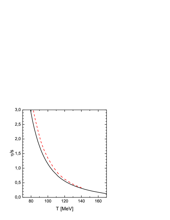
Figure 1: (Color online.) The shear viscosity to entropy density ratio as a function of the temperature for $\mu_{B}=0$. The solid line is the result of the given work and the long-dashed line is that for the interacting pion gas [16].

In Fig. 1 we compare the ratio of the shear viscosity to the entropy density at $\mu_{B}=0$, being calculated in the SHMC model of [4] used in the present work, and that computed in recent paper [16] in the model of the interacting pion gas. The results demonstrate rather appropriate overall agreement although in the SHMC-model the relaxation time is evaluated using phenomenological values of the cross sections of particle species and the calculation of the viscosity is performed in the relaxation time approximation, whereas in [16] the cross sections of the processes are computed (but only for pions) and the viscosity of the pion gas is estimated with the help of the Kubo formalism. This agreement might be considered as an additional argument in favor of estimates of the relaxation time used in [4] and in the given work for $\mu_{B}=0$ and $T\stackrel{{\scriptstyle\scriptstyle<}}{{\phantom{}{}_{\sim}}}150$ MeV, when pions are dominating species.

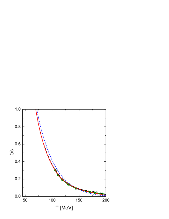
Figure 2: (Color online.) The ratio of the bulk viscosity to the entropy density as a function of temperature at $\mu_{B}=0$. The solid line is the result of the given work, where $\zeta$ satisfies Eq. (32); the short-dashed line is taken from [4], where $\zeta$ fulfills Eq. (24); and the long-dashed line is the result of [5], with $\zeta$ satisfied Eq. (40). The circles present the linear sigma model [17].

In Fig. 2, we show the bulk viscosity to the entropy density ratio at $\mu_{B}=0$ as a function of the temperature. The solid line is calculated in the given work following Eq. (32), model II. The long-dashed curve is the result of Eq. (40) (our model III) derived with the ansatz [5]. In order to perform this calculation we replaced the exact $E$ with the local equilibrium value $E^{\rm l.eq.}$ in (40). The short-dashed curve is our old result [4] calculated following Eq. (24), model I. We see that all three results (especially those calculated following Eqs. (32) and (40)) are close to each other for temperatures $T\stackrel{{\scriptstyle\scriptstyle<}}{{\phantom{}{}_{\sim}}}150$ MeV. For higher temperatures, deviations become a little bit more pronounced. Comparing our results with those computed recently in the linear sigma model [17] in the crossover region (line with circles in the figure) one may see an overall agreement, although models as well as final expressions used for the bulk viscosities are essentially different.

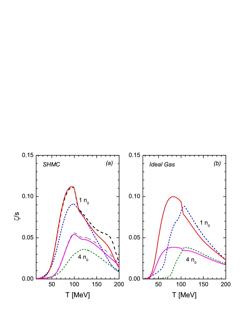
Figure 3: (Color online.) The ratio of the bulk viscosity to the entropy density as a function of temperature for $\mu_{B}\neq 0$, at two values of the baryon density $n_{B}/n_{0}=1$ and $4$ (from top to bottom). Notation is the same as in Fig. 2.

In Fig. 3, the ratio of the bulk viscosity to the entropy density is presented as a function of temperature for two values of the baryon density $n_{B}=n_{0}$ and $4n_{0}$, where $n_{0}=0.16$ fm^-3 is the nuclear density at the saturation point. The notation is the same as in Fig. 2. The results are shown for the SHMC model (a) and for the IG model (b) with the same hadron set. We see that the curves calculated by Eq. (32) and Eq. (40), where we again replaced $E$ with $E^{\rm l.eq.}$, are closer to each other than to the curve calculated with Eq. (24). For the IG, the (solid and long-dashed) curves calculated following Eqs. (32) and (40) coincide. Also, these curves are close to those estimated according to Eq. (24) for $T\stackrel{{\scriptstyle\scriptstyle>}}{{\phantom{}{}_{\sim}}}100$ MeV. Comparing figures (a) and (b) we conclude that the presence of the quasiparticle interaction is more significant for low temperatures ($T\stackrel{{\scriptstyle\scriptstyle<}}{{\phantom{}{}_{\sim}}}100$ MeV) and it becomes less important for higher temperatures.

As we see from Figs. 2 and 3, within our SHMC model all three results (32), (40), and  (24) yield positive values in the temperature-density region of interest. Also we checked positive definiteness of these expressions in case of the ordinary RMF Walecka model by switching off the hadron mass-coupling scaling.

Conclusion. Due to the complexity of the hadron system formed in actual heavy-ion collisions, it is hard to calculate the viscosity coefficients from the first principles with the help of the Kubo formulas. One could use the Kadanoff-Baym kinetic equations for the hadron resonances to derive general expressions for the kinetic coefficients, but at present realistic calculations do not seem possible even in the relaxation time approximation [14]. Therefore, making use of the quasiparticle Boltzmann-like equations (being treated within the relaxation time approximation) can be considered as a forced step for practical evaluations of the kinetic coefficients in the given problem. The scaling hadron mass-couplings model of Ref. [9] is an appropriate tool for the description of the equation of state of the hot and dense hadron system. The knowledge of the latter is necessary in order to perform evaluations of the kinetic coefficients. However, even an application of simplified phenomenological expressions for the relaxation times of different species does not allow one to proceed in calculation of the bulk viscosity without doing additional assumptions, in particular the Landau-Lifshitz conditions should be fulfilled. However, these conditions cannot be satisfied on the class of solutions of the Boltzmann equations for our multi-component system treated within the relaxation time approximation, and additional ansatze are needed. Contrary, the result for the shear viscosity proves to be rather robust to these reductions, see [7].

Thus, we studied three models (models I and III have been previously used in the literature) and derived three expressions for the bulk viscosity (24), (32), and (40), generalized to the case of nonzero chemical potentials $\mu_{B,\,S}$. In derivation of (24) fulfillment of the Landau-Lifshitz conditions is just implied, whereas (32), and (40) fulfill these conditions. Luckily, numerical evaluations, shown in Figs. 2 and 3, carried out following all three expressions deviate not much from each other and confirm earlier results [4, 5, 6, 7, 8]. Although these results can be considered only as rough estimations, Eq. (32) and Eq. (40) seem to be more theoretically justified, while Eq. (24) is less established. In order to perform more accurate calculations, one should go beyond the scope of the relaxation time approximation and fulfill the Landau-Lifshitz conditions on the class of solutions of the kinetic equation. However, such calculations are much more involved than the estimations presented in the given work and have not yet been carried out for multi-component systems with strong interactions.

Acknowledgements. This work was supported by RFBR Grant No. 11-02-01538-a.

References

• [1] J. I. Kapusta, arXiv:0809.3746[nucl-th].
• [2] S. Jeon, Phys. Rev. D 52, 3591 (1995); M. A. Valle Basagoiti, Phys. Rev. D 66, 045005 (2002).
• [3] C. Sasaki and K. Redlich, Phys. Rev. C 79, 055207 (2009).
• [4] A. S. Khvorostukhin, V. D. Toneev, and D. N. Voskresensky, Nucl. Phys. A 845, 106 (2010); Phys. Atom. Nucl. 74, 650 (2011).
• [5] P. Chakraborty and J. I. Kapusta, Phys. Rev. C 83, 014906 (2011).
• [6] A. S. Khvorostukhin, V. D. Toneev, and D. N. Voskresensky, Phys. Rev. C 83, 035204 (2011).
• [7] A. S. Khvorostukhin, V. D. Toneev, and D. N. Voskresensky, Phys. Rev. C 84, 035202 (2011).
• [8] M. Bluhm, B. Kämpfer, and K. Redlich, Phys. Rev. C 84, 025201 (2011).
• [9] A. S. Khvorostukhin, V. D. Toneev, and D. N. Voskresensky, Nucl. Phys. A 791, 180 (2007); A 813, 313 (2008).
• [10] E. E. Kolomeitsev and D. N. Voskresensky, Nucl. Phys. A 759, 373 (2005).
• [11] S. Weinberg, The Quantum Theory of Fields, vol. 1, Cambridge Univ. Press, Cambridge 1995.
• [12] A. Monnai and T. Hirano, Phys. Rev. C80, 054906 (2009), Nucl.Phys. A847, 283 (2010).
• [13] A. A. Abrikosov and I. M. Khalatnikov, Rept. Progr. Phys. 22, 329 (1959).
• [14] D. N. Voskresensky, Nucl. Phys. A 849, 120 (2011).
• [15] S. Gavin, Nucl. Phys. A435, 826 (1985).
• [16] R. Lang, N. Kaiser, W. Weise, Eur. Phys. J. A 48, 109 (2012).
• [17] A. Dobado, J. M. Torres-Rincon, arXiv: 1206.1261 [hep-ph]