Spin and holographic metals

Abstract

In this paper we discuss two-dimensional holographic metals from a condensed matter physics perspective. We examine the spin structure of the Green’s function of the holographic metal, demonstrating that the excitations of the holographic metal are “chiral”, lacking the inversion symmetry of a conventional Fermi surface, with only one spin orientation for each point on the Fermi surface, aligned parallel to the momentum. While the presence of a Kramer’s degeneracy across the Fermi surface permits the formation of a singlet superconductor, it also implies that ferromagnetic spin fluctuations are absent from the holographic metal, leading to a complete absence of Pauli paramgnetism. In addition, we show how the Green’s function of the holographic metal can be regarded as a reflection coefficient in anti-de-Sitter space, relating the ingoing and outgoing waves created by a particle moving on the external surface.

I Introduction

The past few years have seen a tremendous growth of interest in the possible application of “holographic methods”, developed in the context of String theory, to Condensed matter physics. Holography refers to the application of the Maldacena conjecture Maldacena:1997re , which posits that the boundary physics of Anti-de-Sitter space describes the physics of strongly interacting field theories in one lower dimension. The hope is to use holography to shed light on the universal physics of quantum critical metalsNFL-Lee ; NFL-MIT ; NFL-Zaanen . This paper studies the spin character of the holographic metal, showing that its excitations are chiral in character, behaving as strongly spin-orbit coupled excitations with no inversion symmetry and spin aligned parallel to their momentum (see the end of this section).

Quantum criticality refers to the state of matter at a zero temperature second-order phase transition. Such phase transitions are driven by quantum zero-point motion. In contrast to a classical critical point, in which the statistical physics is determined by spatial configurations of the order parameter, that of a quantum critical point involves configurations in space-time with a diverging correlation length and a diverging correlation timesachdevbook ; hertz ; millis . There is particular interest in the quantum criticality that develops in metals, where dramatic departures from conventional metallic behavior, described by Landau Fermi liquid theoryquestions ; gegenwart , are found to develop. Metals close to quantum criticality are found to develop a marked pre-disposition to the development of anisotropic superconductivity and other novel phases of mattermathur ; broun . The strange metal phase of the optimally doped cuprate superconductors is thought by many to be a dramatic example of such phenomenabroun .

In quantum mechanics, the partition function can be rewritten as a Feynman path integral over imaginary time.

$$Z={{\hbox{Tr}}}\left[e^{-\beta H}\right]=\!\int{\cal D}[{\cal O}]\exp\left[-\int_{0}^{\frac{\hbar}{k_{B}T}}d\tau L({\cal O},\tau)\right]$$ (1)

where $L$ is the Lagrangian describing the interacting system and $\tau$ the imaginary time, runs from $0$ to $\hbar/(k_{B}T)$. Inside the path integral, the physical fields ${\cal O}$ are periodic or antiperiodic over this interval. The path integral formulation indicates a new role for temperature: whereas temperature is a tuning parameter at a classical critical point, at a quantum critical point it plays the role of a boundary condition: a boundary condition in timequestions . When a classical critical system is placed in a box of finite extent, it acquires the finite correlation length set by the size of the box. In a similar fashion, one expects that when a quantum critical system with infinite correlation time is warmed to a small finite temperature, the characteristic correlation time becomes the “Planck time”

$$\tau_{T}\sim\frac{\hbar}{k_{B}T}$$ (2)

set by the periodic boundary conditions. This “naive scaling” predicts that dynamic correlation functions will scale as a function of $E/k_{B}T$. Neutron scattering measurements of the quantum critical spin correlations in the heavy fermion systems $CeCu_{6-x}Au_{x}$ and $UCu_{5-x}Pd_{x}$schroeder ; aronson do actually show $E/T$ scaling. The marginal Fermi liquid behavior of the cuprate metals that develops at optimal doping is also associated with such scaling. The most direct approach to quantum criticality, pioneered by Hertzhertz ; millis , in which a Landau Ginzburg action is studied, adding in the damping effects of the metal. Unfortunately, the Hertz approach predicts that naive scaling only develops in antiferromagnets below two spatial dimensions. Today, the origin of $E/T$ scaling in the cuprates and heavy fermion systems, and the many other anomalies that develop at quantum criticality constitutes an unsolved problem. A variety of novel schemes have been proposed to solve this problem, mostly based on the idea that some kind of local quantum criticality emerges qmsi ; varma , but at the present time there is not yet an established consensus. The hope is that holography may help.

Holographic approach

To understand the new approaches, we start with a discussion of the Maldacena conjecture, which proposes that the partition function of a quantum critical (conformally invariant) system can be re-written as a path integral for a higher dimensional gravity (or string theory) problem. In the “physical” system of interest the space-time dimension is $d$ while in the gravity problem there is an extra coordinate $r$ and the space time dimension is $D=d+1$.

The Maldacena conjecture can be written as an identity between the generating functional of a $d$ dimensional conformal field theory, and a $d+1$ dimensional gravity problem, $Z_{\text{CFT}}[j]=Z_{\text{grav}}[\phi]$

$$\left\langle e^{-\int\!\!d^{d}x\ j(x)\,{\cal O}(x)}\right\rangle_{\text{CFT}}=\int D[\phi]\ e^{-\int dr\int d^{d}x\mathcal{L}_{\text{g}rav}[\phi]}$$ (3)

Here $j(x)$ is a source term coupled to the physical field ${\cal O}(x)$, corresponding for instance to a quasi-particle. The right hand side describes the “Gravity dual”, where the gravity fields $\phi(x,r)$ must satisfy the boundary condition that they are equal to the source terms $j(x)$ on the boundary $\lim_{r\rightarrow\infty}\phi(x,r)=j(x)$. This condition establishes the relation between the variables of the d-dimensional field theory and the d+1 dimensional gravity problem in (3). The lower dimensional theory is conformally invariant, which implies that the state is critical in space time, i.e quantum critical. From a condensed matter perspective, the equality of the two sides implies that the physics of the quantum critical system of interest can be mapped onto the surface modes of a higher dimensional gravity problem.

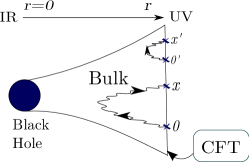
Figure 1: Illustrating the surface excitations “propagating” into the bulk. The horizontal axis is $r$, while the vertical axis is the physical coordinate of the critical theory (CFT).

A physical picture for the AdS coordinate $r$ is obtained as follows. Consider the injection and removal of a particle on the boundary of the AdS space, separated by a distance $x$, as illustrated in fig. 1. When the point of injection and removal are nearby, the Feynman paths connecting them will cluster near the boundary, probing large values of r. By contrast, when the two points are far apart, the Feynman paths connecting them will pass deep within the gravity well of the Anti-de Sitter space, probing small values of $r$ close to the black hole. Hence $r$ represents an energy scale of the problem (corresponding to the ultra-violet cut-off in a renormalization group flow).

The notion that condensed matter near a quantum critical point might acquire a simpler description when rewritten as a gravity dual seems at first surprising, especially considering that the higher dimensional dual is a “string theory” of quantum gravity. The essential simplification occurs in the large $N$ limit. Here, most of the understanding derives from the particular case where the Maldacena conjecture has been most extensively studied and corroborated – a family of $SU(N)$ supersymmetric QCD models with two expansion parameters: a gauge coupling constant $g$ and number of gauge fields $N^{2}$, as summarized in Fig. 2. The corresponding gravity dual, is a string theory with “string coupling constant” $g_{str}$ and a characteristic ratio $l_{str}/L$ between the string length $l_{str}$ and the characteristic length of the space-time geometry where the string resides. While $g_{str}$ controls the amplitude for strings to sub-divide, changing the genus of the world-sheet, $l_{str}$ constrains the amplitude of string fluctuations. The correspondence implies

$$g\sim g_{str},\quad gN\sim(L/l_{str})^{4}$$ (4)

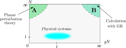
Figure 2: Schematic diagrams for the critical (CFT) theory. Region A can be computed perturbatively on CFT side but is highly non trivial on the string theory side. This paper is about region B where critical theory is strongly correlated but computable with GAR. The real physical models have only $N=1,2$ and $g\sim 1$ and thus are in the center of the diagram.

Each point of fig. 2 has a dual string description. For large $N$ and small $g$ (region A) the critical theory can be computed in perturbation series but a string description is extremely complicated. Some have even suggested this might be way of solving string theory by mapping it onto many body physics Strominger . The focus of current interest in holographic methods is on region B, in the double limit $g,N\rightarrow\infty$, that corresponds to $l_{str}\rightarrow 0$ or just classical gravity. In this sense then, the Maldacena conjecture, if true, provides a new way to carry out large $N$ expansions for quantum critical systems. Since we don’t yet have a working large $N$ theory for quantum critical metals, this may be a useful way of proceeding. A similar philosophy has also been applied in the context of nuclear physics, as a way to place a theoretical limit on the viscosity of quark gluon plasmas Son:2007vk .

The field is at an extraordinary juncture. On the one hand, it is still not known whether the Maldacena conjecture works for a much broader class of models, yet on the other, the assumption that it does so, has led to an impressive initial set of results. In particular, a charged black hole in Anti-de Sitter space appears to generate a strange metal NFL-MIT ; NFL-Lee ; NFL-Zaanen , with a Fermi surface at the boundary of the space and novel anomalous exponents in the self-energy. A fascinating array of results for the strange metals have been obtained, including the demonstration of singlet pairingFaulkner:2009am and even the development of de Haas van Alphen oscillations in the magnetization in an applied fieldDenef:2009yy .

Motivation and results

This paper describes our efforts to understand the ramifications of these developments. One of the motivating ideas was to develop a better physical picture of the strange metal. We were particularly fascinated by the attempt to describe high T_c superconductivity Hartnoll:2008vx ; HartnollBCS (see Horowitz:2010gk for review): in the presence of a charge condensate in the bulk, the boundary strange metal develops a singlet s-wave pair condensate Faulkner:2009am . The formation of singlet s-wave pairs indicates that the strange fermions carry spin, motivating us to ask whether there is a paramagnetic spin susceptibility associated with the strange metal. This led us to examine the matrix spin-structure of fermion propagating in the strange metal.

Spin is a fundamentally three dimensional property of non-relativistic electrons, and in the absence of spin-orbit coupling it completely decouples from the kinetic degrees of freedom as an independent degree of freedom, a common situation in condensed matter physics. By contrast, in the holographic metals studied to date, the particles are intrinsically two dimensional. For these particles, derived from two component relativistic electron spinors, there is no spin. One way to see this is to look at two components of the fermion, which describe the electron and positron fields in two dimensions, leaving no room for spin. How then is it possible to form a spin-singlet superconductor from these fields, when there is no spin to form the singlet?

In this paper, by examining the spin structure of holographic metals we contrast some important similarities and differences between holographic metals and real electron fluids. In our work we have two main results:

1. We show that the excitations of the strange metal are chiral fermions, with spins orientated parallel to the particle momenta. Near the FS the Green’s function becomes

   $$G_{w\rightarrow 0}\ \ ={Z(w)\over{\omega}-v_{F}{\boldsymbol{\sigma}}\cdot{\mathbf{k}}+\Sigma({\omega})}+G_{\text{incoh}}$$ (5)

   The strong spin-momentum coupling generated by the term ${\boldsymbol{\sigma}}\cdot{\mathbf{k}}$ means that the Fermi surface preserves time-reversal symmetry, but violates inversion symmetry. In particular, a simple spin reversal at the Fermi surface costs an energy $2v_{F}k_{F}$, so that the spins are preferentially aligned parallel to the momenta to form chiral fermions. In this way, spin ceases to exist as an independent degree of freedom in two-dimensional holographic metals, as opposed to a spin degenerate interpretation (45). One of the immediate consequences of this result is that the most elementary property of metals, a Pauli susceptibility, is absent.

2. We identify an alternate interpretation of the holographic Green’s functions as the reflection coefficient of waves emitted into the interior of the Anti de Sitter space by the boundary particles, as they reflect off the black hole inside the anti-de Sitter bulk. Namely

   $$G=M_{k}{\cal R}({\omega},{\mathbf{k}})$$ (6)

   where ${\cal R}$ is the reflection coefficient associated with the black hole and $M_{k}$ is a known kinetic coefficient. For bosons $M_{k}=1$ while for fermions $M_{k}=M(\omega,{\mathbf{k}})$ has more involved structure (44). The reflection ${\cal R}$ contains the information about the branch cuts and excitation spectra.

We discuss the full implications of these results in the last section.

II Background Formalism

Our goal is to determine the holographic Green’s functions using linear response theory. Here, for completeness we provide some of the background formal development. For details, we refer the reader to extensive reviewsReview:Hartnoll ; Review:McGreevy ; Review:Liu ; Review:Sachdev .

The main conjecture Maldacena:1997re connecting currents $j$ in lower dimensional CFT and fields of the bulk gravity (as a limit from string theory)

$$Z_{\text{CFT}}[j]=Z_{\text{grav}}[\phi]$$ (7)

where $\phi$ and $j$ are related by the boundary condition

$$j(x)=\lim_{r\rightarrow\infty}\phi(r;x)r^{d-{\Delta}}$$ (8)

the power of $r$ reflects the scaling dimension of the source dim$[j]={\Delta}-d$. The source is coupled to the physical field, better thought as quasi particle, denoted by ${\cal O}(x)$. ${\Delta}$ is the conformal dimension of that field dim$[{\cal O}]={\Delta}$, namely

$$Z_{\text{CFT}}[j]=\left\langle\exp\left[\int d^{d}xj(x){\cal O}(x)\right]\right\rangle_{CFT}.$$

This generating functional determines the physics of the quantum system. The gravity part can be computed classically

$$Z_{\text{grav}}=e^{-S_{\text{grav}}},$$ (9)

derivatives of the generating functional $Z[j]$ determine the Green’s functions of the fields ${\cal O}$

$$\langle{\cal O}\rangle\equiv\left.{{\delta}Z[j]\over{\delta}j}\right|_{j=0}=\lim_{r\rightarrow\infty}{r^{{\Delta}-d}}{{\delta}S_{\rm grav}[\phi]\over{\delta}\phi},$$ (10)

The holographic Green’s functions can be obtain from the quadratic components of the action. The equation of motion then has two independent solutions near the boundary

$$\phi=\underset{\text{\normalsize in-going}}{Ar^{{\Delta}-d}}+\underset{\text{\normalsize out-going}}{Br^{-{\Delta}}}+\ ...\ ,\qquad\text{as }r\rightarrow\infty$$ (11)

Usually the ingoing component $A$ is referred as the “non-normalizable” mode, while the outgoing component $B$ is the “normalizable” mode. Note how the exponents of $r$ match the dimensions of the source and the response ${\cal O}$. In the absence of the source term $j$, the solution must vanish at infinity and the outgoing component vanishes. Once we turn on the source $j$, the Maldacena condition (8) that $\phi(r,x)\rightarrow j(x)$ enables us to identify $A$ as the source

$$j\equiv A.$$

Accordingly, the outgoing mode corresponds to the response $\langle{\cal O}\rangle$

$$\langle{\cal O}\rangle=const\cdot B$$

up to a numerical constant dependent on the particular theory at hand. For a free scalar $const={(2{\Delta}-d})$, for a fermion $const=i{\gamma}^{t}$. In a systematic treatment one needs to regulate the procedure by adding boundary terms, (see appendix A).

Since the Green’s function is the linear response to the source, it follows that up to a constant of proportionality

$$G=const\cdot B/A.$$ (12)

The procedure to extract the Green’s function of a holographic metal is then:

1. Select a background allowing black hole and usually asymptotically AdS.

2. Select the bulk field content and Lagrangian.

3. Select one of the fields with the quantum numbers (spin, charge, etc) of the desired operator ${\cal O}$.

4. Solve the classical field equations in that background, including the backreaction on the gravity.

5. Find the asymptotics of the fields at the boundary. Find the ${\Delta},$ outgoing (leading) and ingoing terms by comparing with (11).

6. The ingoing amplitude at the boundary represents the source, the outgoing amplitude gives the response, the Green’s function is the ratio of the two.

II.0.1 Examples

We now sketch these steps for the scalar and fermion cases. The first step is to choose a background. One of the well known solutions of Einstein-Maxwell equations is the Reissner-Nordström (RN) black hole. This background involves a nontrivial electric field ($E_{r}=-\partial_{r}A_{0}$) and asymptotically AdS metric $g_{\mu\nu}$. In the units where horizon $r=1$, the metric, fields and temperature $T$ are

$$ds^{2}={r^{2}}(-fdt^{2}+dx_{i}^{2})+{1\over r^{2}f}dr^{2},$$ (13)

$$f=1-{Q^{2}+1\over r^{3}}+{Q^{2}\over r^{4}},$$ (14)

$$T={3-Q^{2}\over 4\pi},\qquad A_{0}=\mu\left(1-{1\over r}\right).$$ (15)

Alternate solutions to the metric differ only in the profile function (”blackening factor”) $f(r)$, and the horizons are defined by the zeros of $f(r)$ (as one approaches the horizon time coordinate becomes irrelevant). The solution (13) describes a black hole with electric charge $Q$ in a space with negative cosmological constant. The negative cosmological constant causes the space-time to be asymptotically AdS and thus to have a boundary. The scalar potential $A_{0}$ at the boundary goes to a constant $\mu$, the chemical potential of the boundary theory. Indeed, the RN black hole is a result of steps 1-4 for just one extra field in the bulk, gauge field $A^{\mu}$, which is conjugate to the charge currant operator $\mathcal{J}^{\mu}$. A non-vanishing $A_{0}$ then corresponds to a finite source for $\mathcal{J}^{0}$, which is in fact, the chemical potential $\mu\mathcal{J}^{0}$.

$\bullet$ Bosons. We choose a bulk action

$$S=S_{GR}+S_{EM}+\int d^{4}x(-|\partial\varphi|^{2}-m^{2}|\varphi|^{2})$$ (16)

and the boundary term for a stable solution

$$S_{bnd}=({\Delta}-d)\int_{\partial}d^{3}x\ |\varphi|^{2},$$ (17)

where $S_{GR}+S_{EM}$ is Einstein-Maxwell action. (The term $m^{2}$ can sometimes be slightly negative). In the relativistically invariant measure $d^{d}x$ we have omitted the factor $\sqrt{g}$, where $g$ is the determinant of the metric. This action implies the Einstein-Maxwell equations (solved by the RN black hole background) and free scalar equation. For the boundary terms see the appendix. The Klein Gordon equation in curved space is then

$$(D_{\mu}^{2}+m^{2})\varphi=0,$$ (18)

where

$$D^{2}_{\mu}\equiv D_{\mu}D^{\mu}=(\nabla_{\mu}-iqA_{\mu})(\nabla^{\mu}-iqA^{\mu})=$$

$$=\nabla_{\mu}\nabla^{\mu}-iq\nabla_{\mu}A^{\mu}-2iqA^{\mu}\nabla_{\mu}-q^{2}A^{\mu}A_{\mu}.$$ (19)

Here, the covariant derivative $\nabla_{\mu}$ is defined in terms of the metric, for instance $\nabla^{\mu}\nabla_{\mu}\phi={1\over\sqrt{g}}\partial_{\mu}(\sqrt{g}\,\partial^{\mu}\phi)$, metric $g$ is given in Equation (13). Using a little general relativity and the Fourier transformed $\varphi=\phi\ e^{-iwt+ikx}$ one can write (18) as (m=0)

$$\phi^{\prime\prime}+{(r^{4}f)^{\prime}\over r^{4}f}\,\phi^{\prime}+{(\omega+qA_{0})^{2}-fk^{2}\over r^{4}f^{2}}\,\phi=0.$$ (20)

Now we are to solve the equation to find the asymptotics and identify the ingoing and outgoing modes. Since it is a second order differential equation, the full solution can be found numerically, but the asymptotics at $r\rightarrow\infty$ are easily extracted analytically, using $f(r)\rightarrow 1$.

$$\phi^{\prime\prime}+{4\over r}\,\phi^{\prime}=0$$ (21)

hence

$$\phi=A+Br^{-3}.$$

The leading ingoing term is a constant $A$, hence ${\Delta}=3$, while the outgoing term should be $r^{-{\Delta}}$, cf. (11). To get the proportionality constant we use (10).

$$\langle{\cal O}\rangle=-3B,$$ (22)

so the retarded Green’s function is

$$\quad G=-3B/A$$ (23)

which is actually a $m=0$ case for $G=(2{\Delta}-d)B/A$.

$\bullet$ Fermions. We can introduce the action

$$S=S_{GR}+S_{EM}+S_{\varphi}+\int d^{4}x\ i\ \overline{\psi}({\gamma}^{\mu}D_{\mu}-m)\psi$$ (24)

with $\overline{\psi}=\psi^{\dagger}{\gamma}^{t}$, and the boundary action

$$S_{bnd}=\int_{\partial}d^{3}x\ \overline{\psi}\psi.$$ (25)

The main difference now is the fact that a fermion in 4 dimensions has four components: four quantum-mechanical degrees of freedom (simply spin up, spin down, electron, positron) but the boundary fermion has only 2 components. Thus the other half of the components should not play a role. Without loss of generality the mass m is positive. In the addition to the Einstein-Maxwell equation this action also implies the Dirac equation

$$({\gamma}^{\mu}D_{\mu}-m)\psi=0$$ (26)

Before the next step we rewrite (26) in its full form:

$$(\sqrt{g^{rr}}{\Gamma}^{r}\partial_{r}-i\sqrt{g^{00}}{\Gamma}^{0}w+i\sqrt{g^{ii}}{\Gamma}^{i}k_{i}-m)\psi=0$$ (27)

$$\text{with:}\quad w=\omega+qA_{0}$$

As in the scalar case, to determine Green’s function, we examine the asymptotics boundary behavior, $r\rightarrow\infty$. In our basis

$$\begin{pmatrix}m+r\partial_{r}&i{{\gamma}^{\mu}k_{\mu}\over r}\\ i{{\gamma}^{\mu}k_{\mu}\over r}&m-r\partial_{r}\end{pmatrix}{\psi_{+}\choose\psi_{-}}=0,$$ (29)

here $k^{\mu}=(w,{\mathbf{k}})$. This is a $4\times 4$ matrix equation with the following solution.

$$\psi\rightarrow r^{-\frac{3}{2}}\left(\begin{array}[]{c}\psi_{+}\\ \psi_{-}\end{array}\right);\quad\left\{\begin{array}[]{c}\psi_{+}=Ar^{m}+Dr^{-m-1}\\ \psi_{-}=Br^{-m}+Cr^{m-1}\end{array}\right.$$ (30)

From the four terms we choose in- and out-going modes in an analogous fashion to the scalar case, the leading term $Ar^{m-3/2}$ is in-going, while the term $Ar^{-m-3/2}$ is outgoing and the dimension is

$${\Delta}=m+3/2.$$ (31)

The other terms ($C,D$) are related to the first two. To determine this dependence we need to substitute the asymptotics back into the Dirac equation (26), which leads to

$$B={2m+1\over i{\gamma}^{\mu}k_{\mu}}D.$$ (32)

As in (23) the Green’s function can be expressed in terms of $A$’s and $B$’s (note $A$ and $B$ are spinors):

$$GA=i{\gamma}^{t}B.$$ (33)

As before, we obtain the coefficient $i{\gamma}^{t}$ by taking a derivative of the action and ${\gamma}^{t}$ is a part of the definition of $\overline{\psi}$. Armed with (32)

$$GA={\gamma}^{t}{2m+1\over{\gamma}^{\mu}k_{\mu}}D\equiv M_{k}D.$$ (34)

III Reflection Approach

In the previous section we made use of the ingoing/outgoing terminology. In this section we identify these modes explicitly. Here we show how to redefine the problem in a form resembling the quantum mechanics of a reflected wave. This can be done by transforming coordinates according to $ds=F(r)dr$ and rescaling the wave function as $\psi(r)=Z(r)\Psi(s)$. The original equation then becomes a zero energy scattering problem

$$(\partial_{s}^{2}-V)\Psi(s)=0,$$ (35)

with a complicated and non-unique function $V(s)$. (The retarded Green’s function must be derived using an infalling boundary condition at the black hole horizon Son:2002sd . An advantage of this approach is that the infalling wave condition is derived as immediate consequence of the scattering problem.)

Bosons. Consider again the scalar probe Equation of motion (21) in the RN black hole geometry, defined in (13-15). The generalization to the full backreacting solution is straightforward. The rescaling of coordinates and fields $\varphi(r)\rightarrow\phi(s)$

$$ds=Fdr,\ \ \ \ \varphi=Z\phi$$ (36)

leads to the following

$$(\partial_{r}^{2}+D_{1}\partial_{r}+D_{0})\varphi\rightarrow$$

$$(\partial_{s}^{2}+{D_{1}+\frac{F^{\prime}}{F}+\frac{2Z^{\prime}}{Z}\over F}\partial_{s}+{D_{0}+\frac{Z^{\prime\prime}}{Z}+D_{1}\frac{Z^{\prime}}{Z}\over{F^{2}}})\phi=0.$$

There are an infinite number of ways to tune equation (21) to the form of the Schrodinger equation by canceling $\partial_{s}\phi$ term. We will choose the non-unique combination

$$F=i/fr,\qquad Z=1/r^{3/2}.$$ (37)

This leads to the zero energy scattering problem $\partial_{s}^{2}\phi-V(s)\phi=0$ with potential given by

$$V(r)={w^{2}-k^{2}f-m^{2}fr^{2}\over r^{2}}-f^{2}\left(\frac{9}{4}+\frac{3f^{\prime}}{2rf}\right)$$ (38)

It is useful to write the limiting values of this potential. It turns out that it goes to a constant on both the horizon and the boundary.

$$V(r\rightarrow\infty)=-m^{2}-{9/4},\quad V(r\rightarrow\text{horizon})=\omega^{2}$$ (39)

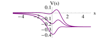
Figure 3: Typical Schrodinger potential $m^{2}=-2,\ \ Q^{2}=3,\ k={1,1.6,2},\ \omega=0$ (from the top). The incoming wave propagates from the right with zero energy.

Finally, we reformulate the Green’s Function as a reflection coefficient. Namely

$$\phi(r\rightarrow\infty)=A\left(e^{is(\Delta-3/2)}+{\cal R}e^{-is(\Delta-3/2)}\right)$$ (40)

leading to

$$G(\omega,k)={\cal R}$$ (41)

Fermions in this case the reflection coefficient becomes a matrix. We have already written the Dirac equation in the black hole background (29). One can ”square’ the first order $4\times 4$ matrix equation to obtain a second order $2\times 2$ equation. After rescaling the fields in the same fashion as in the scalar case, the potential acquires the same form as in the scalar case in fig. 3, but with the different limits

$$V(r\rightarrow\infty)=-(m+1/2)^{2},\quad V(r\rightarrow\text{horiz.})=\omega^{2}.$$ (42)

As in (40) the solution is a superposition of incident and reflected waves:

$$\psi_{+}\rightarrow\left(e^{is(m+\frac{1}{2})}+{\cal R}e^{-is(m+\frac{1}{2})}\right)A,$$ (43)

where the reflection coefficient ${\cal R}$ is now a matrix. The Green’s function is proportional to ${\cal R}$ up to a kinematic factor $M_{k}$

$$G=M_{k}{\cal R}={2m+1\over(\omega+q\mu)-{\boldsymbol{\sigma}}\cdot{\mathbf{k}}}{\cal R}.$$ (44)

Here we use equation (34). However suggestive the form of $M_{k}$ is, its poles do not affect the physical non-analyticities of the Green’s function G: it is ${\cal R}$ which contains all the relevant poles and branch cuts.

IV Spin structure

We now return to the question of the spin character of the holographic fermion. In quantum critical metals, the spin degree of freedom plays an essential role. For example, the application of a magnetic field, via the Zeeman coupling, allows one to tune the system through a quantum critical point. The presence of critical spin fluctuations is thought to play an important role in break-down of Landau Fermi liquid behavior. This then raises the question as to whether the holographic fermions obtained by projection from four-dimensional anti-de-Sitter space, carry a spin quantum number. Furthermore, what is the nature of the soft modes that drive the quantum criticality, and is it possible to gap these modes, driving a transition back into a Fermi liquid? The boundary fermions that form about a $D=4$ anti-de-Sitter space are Dirac fermions described by a two component spinor. Hartnoll at al Hartnoll:2008vx have shown that when a condensed Bose field is introduced into the bulk gravity dual, these Fermi fields form s-wave, singlet pairs. This establishes that the fermions do indeed carry spin, however, as we shall now show, this spin is “chiral”${}^{\text{\ref{footnote2}}}$ and is aligned rigidly with the momentum of the excitation at the Fermi surface. There is no inversion symmetry, and at each point on the Fermi surface there is a single spin polarization. However, time reversal is not broken, and reversing the spin also implies reversing the momentum, so it is still possible to form pairs by combining fermions with opposite spin on opposite sides of the two dimensional Fermi surface.

It is often tacitly assumed that the excitations of holographic metals are non-relativistic fermions, with an independent spin degree of freedom. In this case the Green’s function $G_{{\alpha}{\beta}}={\delta}_{{\alpha}{\beta}}G$ would be proportional to the unit operator as in Polchinski

$$G_{{\alpha}{\beta}}={\delta}_{{\alpha}{\beta}}{1\over\omega-v_{F}(k-k_{F})-g^{2}\Sigma}$$ (45)

Here we shall argue that this is not the case and the spin-orbit coupling remains very large in holographic metals despite the formation of a Fermi surface, forcing the spin to align with the momentum.

First consider the relativistic case without the black hole when the surface excitations are undoped and form a strongly interacting Dirac cone of excitations with Lorentz invariance. The corresponding Lorentz invariant correlation function is $\langle{\cal O}\bar{{\cal O}}\rangle^{-1}=\tilde{C}k_{\mu}{\gamma}^{\mu}$, where $\bar{{\cal O}}={\cal O}^{\dagger}{\gamma}^{0}$ and $\tilde{C}$ is an arbitrary function of 3-momentum $k=\sqrt{\omega^{2}-{\mathbf{k}}^{2}}$ . For non-relativistic applications we are interested in $\langle{\cal O}{\cal O}^{\dagger}\rangle$ and we turn to a Hamiltonian formalism, treating time and space separately. The Green’s functions takes the form $G^{Lor}=\langle{\cal O}{\cal O}^{\dagger}\rangle=-\langle{\cal O}\bar{{\cal O}}\rangle{\gamma}^{0}$

$$G^{Lor}(\omega,{\mathbf{k}})=[\tilde{C}(k)({\mathbf{k}}\cdot{\boldsymbol{\sigma}}-{\omega})]^{-1}.$$ (46)

For the case of zero bulk fermion mass $\tilde{C}(k)=1/k$. Here we have introduced the Pauli matrixes $\sigma^{i}={\gamma}^{i}{\gamma}^{0}$, for $i=1,2$. Eq. (46) describes two Dirac cones as depicted on fig.4-a, where upper and lower cones have the opposite chirality. There is only one spin orientation parallel to the momentum at any given energy.

Figure 4: Typical dispersion and Fermi surface of Dirac fermion in 2+1 (a); and the holographic metal from fig.6-a (b).

Once we add a charged black-hole, the boundary excitations are “doped”, acquiring a finite Fermi surface (and Fermi velocity $v_{F}$) that breaks the Lorentz invariance down to a simple rotational invariance. The only rotationally invariant way in which spin can enter, is in the form of a scalar product with the momentum ${\mathbf{k}}\cdot{\boldsymbol{\sigma}}$. The most general Green’s function now takes the form

$$G(\omega,{\mathbf{k}})=[C_{1}(\omega,k){\mathbf{k}}\cdot{\boldsymbol{\sigma}}+C_{2}(\omega,k)]^{-1}$$ (47)

where $C_{1}$ and $C_{2}$ are two arbitrary functions which depend on the frequency $\omega$ and the magnitude of the non-relativistic momentum $k=|{\mathbf{k}}|$.

The physical properties of the theory depend on the form of the coefficients $C_{1,2}$. For example, if $C_{1}=0$, then the Fermi surface would be spin degenerate (${\boldsymbol{\sigma}}$ independent). If $C_{1}$ is finite and purely real, the momentum becomes strongly coupled to the spin via ${\mathbf{k}}\cdot{\boldsymbol{\sigma}}$ (spin flip does change the ground state) and we are dealing with chiral excitations. One can interpret $C_{1}$ as a wave-function renormalization: $C_{1}=v_{F}Z^{-1}$ and $C_{2}$ as a self energy: $C_{2}=Z^{-1}({\omega}+\Sigma-\mu)$. However, if $C_{1}$ has an imaginary part, while the chiral property remains, spin flips become highly incoherent in nature, so a standard decomposition of the quasiparticle along the lines of the electron phonon problem is not possible.

To bring out the chiral ($C_{1}\neq 0$) properties we introduce the chirality projection operators

$$\Pi_{\pm}=\frac{1}{2}\left(1\pm{{\mathbf{k}}\cdot{\boldsymbol{\sigma}}\over k}\right),$$ (48)

which leads to

$$G=\Pi_{+}G_{11}+\Pi_{-}G_{22},$$ (49)

where $G_{11}$ and $G_{22}$ are the eigenvalues of the matrix $G$ and $2kC_{1}=G_{11}^{-1}-G_{22}^{-1}$, $2C_{2}=G_{11}^{-1}+G_{22}^{-1}$.

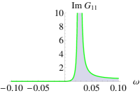
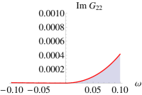
Figure 5: Typical behavior of a spectral function $\pi A({\omega},k)={\rm Im\,}G_{11}+{\rm Im\,}G_{22}$ at fixed momentum $k=k_{F}+10^{-2}$. ${\rm Im\,}G_{11}$ has a spike that sharpens for $k\rightarrow k_{F}$ and ${\rm Im\,}G_{22}$ is suppressed. Snapshot for RN black hole with $q=2$, $m=-1/5$.

Fig. 5 illustrates a typical numerical solution for the eigenvalues. ${\rm Im\,}{G_{ii}}$ is plotted for fixed $k$ close to the Fermi surface. One eigenvalue has a peak, which we interpret as the chiral quasiparticle component to the spectral function while the other, corresponding to the incoherent background created by flipping the spin anti-parallel to the momentum, lacks any sharp features and goes to zero at the Fermi surface. The spectral function $A({\omega},{\mathbf{k}})=\frac{1}{\pi}{\rm Im\,}{\hbox{Tr}}G$ is${}^{\text{\ref{footnote1}}}$

$$A({\omega},{\mathbf{k}})=\frac{1}{\pi}{\rm Im\,}[G_{\text{chiral}}(\omega,{\mathbf{k}})+G_{\text{incoh}}(\omega,{\mathbf{k}})],$$ (50)

where $G_{\text{chiral}}$ refers to the coherent part of the resonance and $G_{\text{incoh}}$ is the incoherent background.

To further emphasize the chiral structure we use an analytic form of the Green’s function. Near $k=k_{F}$ and $\omega\rightarrow 0$ this can be obtained Faulkner:2009wj by matching the infra-red ’inner’ region of the RN black hole to the asymptotic AdS ’outer’ region.

$$G_{11}={z\over{\omega}-v_{F}(k-k_{F})+c_{1}{\omega}^{2\nu}},$$ (51)

where $z,v_{F}$ are real and $c_{1}$ is a complex constant. The exponent $\nu\equiv\sqrt{m^{2}+k_{F}^{2}-q^{2}/2}/\sqrt{6}$ depends on the mass and the charge of the fermion. Armed with (49) we arrive to

$$G\ ={z\over\omega-v_{F}({\mathbf{k}}\cdot{\boldsymbol{\sigma}}-k_{F})+c_{1}{\omega}^{2\nu}}+G_{incoh}$$ (52)

Finally it is interesting to find a dispersion for the quasi-particle: the line where the real part of the inverse G-function is zero, ${\rm Re\,}\,G^{-1}=0$. Since the imaginary part is zero only at ${\omega}=0$, the fermi surface is the intersection of the two lines. The results are illustrated in fig. 6. The case of a massless fermion is particularly interesting, we see that the dispersion relation actually follows a parabolic form $\sqrt{p^{2}+(m^{*})^{2}}$ showing that the holographic fermion running around the doped black hole has developed a finite effective mass $m^{*}$. The dispersion at the Fermi surface is very similar to the linear dispersion of chiral fermion.

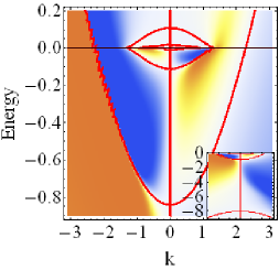
(a)  $m=0$

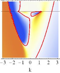
(b)  $m=-1/10$

Figure 6: Density plot of ${\rm Re\,}G^{-1}$. The zeros of the inverse Green’s function represent the quasi-particle dispersion and are depicted by the red line (the wavy line indicates discontinuities). Left panel: $m=0$. Right panel: $m=-0.1$. The dispersion crosses through the Fermi wavevector at zero energy. (The inset: lower energy range is shown. As in fig.4-b, there is a dispersion branch with a different effective mass $m^{*}$)

Summarizing the main points:

• The Fermi Surface is rotationally invariant and has a single non-degenerate fermionic excitation at every momenta,

• The spin of the coherent excitations lies parallel to the momentum as shown in figure 4, giving rise to chiral quasi-particle interpretation,

• The incoherent background is generated by a spin-flip of a coherent chiral quasiparticle.

V Discussion

The possible application of holographic methods to condensed matter physics AdSCMT is based in part on a dream of a deep universality: the idea that the scale-invariance of quantum criticality in metals might enjoy the same level of universality seen in statistical physics.

Nevertheless, there is still a huge gulf to be crossed. From a String theory perspective, there is still a need to show that semi-classical gravity metric used in the theories emerges as a consistent truncation of string theory on a certain “brane” configuration. From a condensed matter perspective, we lack a systematic method to constructing an AdS dual: one encouraging direction may be to map the renormalization group flows of the quantum theory onto a higher dimension Lee:2012 .

Against this backdrop, the field has taken a more pragmatic approach of simply exploring the holographic consequences of anti-de-Sitter space, assuming that all is well. One can not fail to be impressed by the discovery that a charged black hole nucleates a strange metal on its surface, with properties that bear remarkable similarities to condensed matter systems: the emergence of a critical Fermi surface with quantum oscillations, the presence of E/T scaling, Pomeranchuk instabilities Pomeranchuk and even the phase diagram of type II superconductors type2 .

Our interest in the field was sparked by a naive impression that progress in holography resembles the history of condensed matter physics “running in reverse”! Rather than starting with the simple Pauli paramagnetic metal and building up to an understanding of Fermi liquids and ultimately quantum criticality, holography appears to start with the critical Fermi surface, working backwards to the most basic elements of condensed matter physics. This led us to ask, whether one calculate the most elementary property of all, the Pauli susceptibility in response to a Zeeman splitting.

Our work has provided a interpretation of the holographic Green’s function as a momentum and frequency dependent reflection coefficient of waves emitted by surface particles, reflected off the horizon of the interior black hole. We have also shown that the excitations of the strange metal are intrinsically chiral, with spins locked parallel to the momentum by a strong spin-orbit coupling with no inversion symmetry. The situation is reminiscent to the surface of 3D topological insulator.

This observation means in fact, that there is no Pauli susceptibility of the two dimensional holographic metal: the Fermi sea is already severely polarized by the relativistic coupling between momentum and spin. Indeed, from a physical perspective, the strange metallic behavior seen in these systems would appear to be a consequence of soft charge or current fluctuations rather than spin fluctuations. In recent work Faulkner:2009am , Faulkner et al have discovered that when a charge gap is introduced by condensing a boson in the AdS bulk, the holographic metal develops sharp Fermi-liquid-like quasiparticles. This is consistent with this interpretation.

Spin plays a major role in the quantum criticality of condensed matter. In many systems, the application of a field, via the Zeeman splitting is the method of choice for tuning through criticality YRS ; Ybal1 . Clearly, this part of the physics is inaccessible to the current approach. The absence of a Zeeman-splitting in holographic metals was first observed by adding a monopole charge to the black hole Albash:2009wz ; Basu:2009qz .

Various authors have explored the possibility of introducing spin as an additional quantum number. The simplest example is the ”magnetically charged” black hole, with an “up” and a “down” charge to simulate the Zeeman splitting, coupling to the fermions via a “minimal coupling” (a spin-dependent vector potential)Iqbal:2010eh . By construction, this procedure does produce an explicit “Zeeman” splitting of the Fermi surface, however the infra-red character of the problem, described by the interior geometry of the gravity dual, is unchanged and the strange metal physics of the “up” and “down” Fermi surfaces are essentially unaffected by the magnetic field.

An alternative approach might be to introduce the Zeeman term to the holographic metals by invoking a non-minimal coupling to electromagnetic field, akin to the anomalous magnetic coupling of a neutron or proton. A number of recent papers have considered the effect of such terms in the absence of a magnetic field, where they play the role of anomalous dipole coupling termsdipole1 ; dipole2 . At strong coupling these terms have been found to inject a gap into the fermionic spectrum interpreted as a Mott gapdipole2 . However, when a monopole charge is added to the black hole to generate a magnetic coupling to these same terms, we find they do not generate a splitting of the chiral Fermi surface, nor do they change the interior geometry of the gravity dual. The construction of a holographic metal with non-trivial spin physics may require considering 3-dimensional holographic metals projected out of 4+1 dimensional gravity dual Kraus , where the additional dimensionality permits four-component fermionic fields with both left and right-handed chiralities.

Note: Shortly before posting our paper, a related work by Hertzog and RenHerzog appeared with results that compliment those derived here. These authors concentrate on the behavior of gravity duals with a large black-hole charge and a non-zero fermion mass, a limit where the holographic metal contains multiple Fermi surfaces. They find that in this limit, in addition to a Rashba component ${\boldsymbol{\sigma}}\cdot(\hat{z}\times{\mathbf{k}})$ the dispersion of the holographic metal also develops a quadratic spin-independent dispersion reminiscent of more weakly spin-orbit coupled fermions. The Rashba term ${\boldsymbol{\sigma}}\cdot(\hat{z}\times{\mathbf{k}})$ obtained by Herzog and Ren is equivalent to the helicity term ${\boldsymbol{\sigma}}\cdot{\mathbf{k}}$ described in our paper after a rotation of spin axes. In the limit of small black-hole charge considered here, with a single Fermi surface, the helicity term in the Hamiltonian entirely dominates the spectrum.

Acknowledgments.

We gratefully acknowledge discussions with Steve Gubser, Matt Strassler, Scott Thomas and Yue Zhao. This work was supported by National Science Foundation grant DMR 0907179.

Appendix A Boundary terms

The general idea of holographic renormalization Skenderis:2002wp is to add boundary terms to the classical gravity action. This terms simply make sure that all sensible physical quantities are finite. Good examples of such quantities are the total energy of the bulk (mass of a black hole inside) and the entropy. Those have nothing to do with duality and in some cases were introduces long before it, for instance by Hawking in 70’s to actually make sense of his famous black hole temperature calculation. In AdSCFT it is useful to think about stability of a given AdS solution.

The Dirac action for fermions in the bulk is of the form

$$S=i\int d^{d+1}x\sqrt{g}\ \overline{\psi}({\gamma}^{\mu}D_{\mu}-m)\psi$$ (53)

in the bulk $\psi_{+}$ and $\psi_{-}$ are related through each other momenta, but the conjugate momenta for $\overline{\psi}_{+}$ is zero:

$$\Pi_{+}=-\sqrt{\frac{g}{g_{rr}}}\psi_{-}\quad\text{but }\quad\overline{\,\Pi}_{+}=0$$ (54)

Which is unphysical since we expect both momenta to represent a physical degree of freedom. The naive way to fix it which turns out to be the correct one is to change the bulk action by symmetrizing the kinetic term: split the derivative in half. One is acting to the left (represented by the arrow) and another is to the right.

$$S\rightarrow\frac{i}{2}\int d^{d+1}x\sqrt{g}\ \overline{\psi}({\gamma}^{\mu}\overrightarrow{D}_{\mu}-{\gamma}^{\mu}\overleftarrow{D}_{\mu}-2m)\psi$$ (55)

which is different from the original action by a boundary term

$${\delta}S_{\rm bound}=\int_{\partial}d^{d}x\ \sqrt{\frac{g}{g_{rr}}}\ \ \overline{\psi}_{+}\psi_{-}+h.c.$$ (56)

And we are back to equation (25). We refer to Henningson:1998cd for more details.

References

- (1) J. M. Maldacena, “The large N limit of superconformal field theories and supergravity,” Adv. Theor. Math. Phys. 2, 231 (1998)
- (2) S. -S. Lee, “A Non-Fermi Liquid from a Charged Black Hole: A Critical Fermi Ball,” Phys. Rev. D 79, 086006 (2009)
- (3) H. Liu, J. McGreevy and D. Vegh, “Non-Fermi liquids from holography,” Phys. Rev. D 83, 065029 (2011)
- (4) M. Cubrovic, J. Zaanen and K. Schalm, “String Theory, Quantum Phase Transitions and the Emergent Fermi-Liquid,” Science 325, 439 (2009)
- (5) S. Sachdev, “Quantum Phase Transitions”, Cambridge University Press, Second Edition (2011).
- (6) J. A. Hertz, “Quantum critical phenomena”, Phys. Rev. B 14, 1165 (1976).
- (7) A. J. Millis, “ffect of a nonzero temperature on quantum critical points in itinerant fermion systems.”, Phys. Rev. B 48, 7183 (1993).
- (8) P. Coleman, C. Pé́pin, Q. Si, and R. Ramazashvili, “How do Fermi liquids get heavy and die?”, J. Phys. Condens. Matter 13, R723–R738 (2001).
- (9) P. Gegenwart, Q. Si and F. Steglich, “Quantum Criticality in Heavy Fermion Metals”, Nature Physics, 4, 186 (2008).
- (10) N. Mathur et al., “Magnetically mediated superconductivity in heavy fermion compounds” Nature 394,39 (1998).
- (11) D. M. Broun, “What lies beneath the dome”, Nature Physics, 4, 170, (2008).
- (12) A. Schroeder et al., “Onset of antiferromagnetism in heavy-fermion metals”, Nature 407, 351(2000).
- (13) M.C. Aronson, R. Osborn, R.A. Robinson, J.W. Lynn, R. Chau, C.L. Seaman, and M.B. Maple, “Non-Fermi-Liquid Scaling of the Magnetic Response in UCu 5-xPdx(x = 1,1.5)”, Phys. Rev. Lett. 75, 725 (1995).
- (14) Q. Si, S. Rabello, K. Ingersent and J.L. Smith, “Locally critical quantum phase transitions in strongly correlated metals” Nature 413 804 (2001)
- (15) C. M. Varma, P. B. Littlewood, S. Schmitt-Rink, E. Abrahams, and A. E. Ruckenstein, “Phenomenology of the normal state of Cu-O high-temperature superconductors”, Phys. Rev. Lett. 63, 1996 (1989)
- (16) A. Strominger, “Black hole entropy from near horizon microstates,” JHEP 9802, 009 (1998)
- (17) D. T. Son, A. O. Starinets, “Viscosity, Black Holes, and Quantum Field Theory,” Ann. Rev. Nucl. Part. Sci. 57, 95 (2007).
- (18) T. Faulkner, G. T. Horowitz, J. McGreevy, M. M. Roberts and D. Vegh, “Photoemission ’experiments’ on holographic superconductors,” JHEP 1003, 121 (2010)
- (19) F. Denef, S. A. Hartnoll and S. Sachdev, “Quantum oscillations and black hole ringing,” Phys. Rev. D 80, 126016 (2009)
- (20) S. A. Hartnoll, C. P. Herzog and G. T. Horowitz, “Building a Holographic Superconductor,” Phys. Rev. Lett. 101, 031601 (2008)
- (21) T. Hartman and S. A. Hartnoll, “Cooper pairing near charged black holes,” JHEP 1006, 005 (2010)
- (22) G. T. Horowitz, “Introduction to Holographic Superconductors,” arXiv:1002.1722 [hep-th].
- (23) S. A. Hartnoll, “Lectures on holographic methods for condensed matter physics,” Class. Quant. Grav. 26, 224002 (2009)
- (24) J. McGreevy, “Holographic duality with a view toward many-body physics,” Adv.High Energy Phys. 2010 723105 (2010)
- (25) N. Iqbal, H. Liu and M. Mezei, “Lectures on holographic non-Fermi liquids and quantum phase transitions,” arXiv:1110.3814 [hep-th].
- (26) S. Sachdev, “What can gauge-gravity duality teach us about condensed matter physics?”, Annual Rev. Cond. Mat. Phys. 3, 9 (2012)
- (27) P. Breitenlohner and D. Z. Freedman, “Positive energy in Anti-de Sitter backgrounds and gauged extended supergravity,” Phys. Lett. B115 (1982) 197.
- (28) D. T. Son and A. O. Starinets, “Minkowski-space correlators in AdS/CFT correspondence: Recipe and applications,” JHEP 0209, 042 (2002)
- (29) T. Faulkner and J. Polchinski, “Semi-Holographic Fermi Liquids,” JHEP 1106, 012 (2011)
- (30) T. Faulkner, H. Liu, J. McGreevy and D. Vegh, “Emergent quantum criticality, Fermi surfaces, and AdS(2),” Phys. Rev. D 83, 125002 (2011)
- (31) S. -S. Lee, “Background independent holographic description : From matrix field theory to quantum gravity,” arXiv:1204.1780 [hep-th].
- (32) M. Edalati, K. W. Lo and P. W. Phillips, “Pomeranchuk Instability in a non-Fermi Liquid from Holography,” arXiv:1203.3205 [hep-th].
- (33) S. A. Hartnoll, C. P. Herzog and G. T. Horowitz, “Holographic Superconductors,” JHEP 0812, 015 (2008)
- (34) J. Custers, P. Gegenwart, H. Wilhelm, K. Neumaier, Y. Tokiwa, O. Trovarelli, C. Geibel, F. Steglich, C. Pépin and P. Coleman, ”Break up of the heavy electron at a quantum critical point” Nature, 424, 524 (2003).
- (35) S. Nakatsuji et al., “Superconductivity and quantum criticality in the heavy-fermion system -YbAlB4”. Nat. Phys. 4, 603 (2008)
- (36) T. Albash and C. V. Johnson, “Holographic Aspects of Fermi Liquids in a Background Magnetic Field,” J. Phys. A 43 (2010) 345405
- (37) P. Basu, J. He, A. Mukherjee and H. -H. Shieh, “Holographic Non-Fermi Liquid in a Background Magnetic Field,” Phys. Rev. D 82, 044036 (2010)
- (38) N. Iqbal, H. Liu, M. Mezei and Q. Si, “Quantum phase transitions in holographic models of magnetism and superconductors,” Phys. Rev. D 82, 045002 (2010)
- (39) M. Edalati, R. G. Leigh and P. W. Phillips, “Dynamically Generated Mott Gap from Holography,” Phys. Rev. Lett. 106, 091602 (2011)
- (40) D. Guarrera, J. McGreevy, “Holographic Fermi surfaces and bulk dipole couplings,” [arXiv:1102.3908 [hep-th]].
- (41) E. D’Hoker and P. Kraus, “Holographic Metamagnetism, Quantum Criticality, and Crossover Behavior,” JHEP 1005, 083 (2010)
- (42) K. Skenderis, “Lecture notes on holographic renormalization,” Class. Quant. Grav. 19, 5849 (2002)
- (43) M. Henningson and K. Sfetsos, “Spinors and the AdS/CFT correspondence,” Phys. Lett. B 431, 63 (1998)
- (44) C. P. Herzog and J. Ren, “The Spin of Holographic Electrons at Nonzero Density and Temperature,” arXiv:1204.0518 [hep-th].