Virus Replication as a Phenotypic Version of Polynucleotide Evolution

Abstract

In this paper we revisit and adapt to viral evolution an approach based on the theory of branching process advanced by Demetrius, Schuster and Sigmund (“Polynucleotide evolution and branching processes”, Bull. Math. Biol. 46 (1985) 239–262), in their study of polynucleotide evolution. By taking into account beneficial effects we obtain a non-trivial multivariate generalization of their single-type branching process model. Perturbative techniques allows us to obtain analytical asymptotic expressions for the main global parameters of the model which lead to the following rigorous results: (i) a new criterion for “no sure extinction”, (ii) a generalization and proof, for this particular class of models, of the lethal mutagenesis criterion proposed by Bull, Sanjuán and Wilke (“Theory of lethal mutagenesis for viruses”, J. Virology 18 (2007) 2930–2939), (iii) a new proposal for the notion of relaxation time with a quantitative prescription for its evaluation, (iv) the quantitative description of the evolution of the expected values in in four distinct “stages”: extinction threshold, lethal mutagenesis, stationary “equilibrium” and transient. Finally, based on these quantitative results we are able to draw some qualitative conclusions.

1 Introduction

RNA viruses exhibit a pronounced genetic diversity (Domingo and et al., 1985). This variability allows RNA virus to better adapt to environmental challenges as represented by host and therapy pressures (Domingo et al, 1998). Due to the lack of a proofreading activity of viral RNA polymerases (average error incorporation rate of order $10^{-4}$ per nucleotide, per replication cycle (Steinhauer et al, 1992)), short generation times and huge population numbers, RNA viral populations may be viewed as a collection of particles bearing mutant genomes.

As a consequence of high mutation rates, frequencies of mutants depend not only on their level of adaptation but on the probability of being faithfully replicated during viral genomic RNA synthesis. Several studies (Domingo et al, 1998; Elena and Sanjuán, 2005) have looked at viral diversification processes as a contributing cause of disease progression and of therapeutic strategies shortcomings including vaccine trials. It has become important to understand the process by which virus acquire diversity and the dynamics and fluctuations of this diversity in time. However, understanding viral evolution in vivo has proven to be a very unwieldy accomplishment due to the huge number of variables involved in the interplay between viruses and their hosts.

For the last 30 years, quasi-species theory has provided a population-based framework to model RNA viral evolution. Quasi-species theory is a mathematical framework that was initially formulated to explain the evolution of macromolecules (Eigen, 1971). More recently, it has been used to describe the evolutionary dynamics of RNA viruses. However, quasi-species theory is based on deterministic equations and so has a number of serious drawbacks when applied to realistic experimental systems since there are important sources of stochasticity that must be taken into account.

Traditionally, in an effort to make the viral evolution process more palpable, several groups have addressed this subject from different points of view. There is a substantial amount of publications that studied virus populations during their evolution in experimental settings, for instance, cell cultures (Escarmís et al, 2006), by challenging the virus with population bottlenecks (Ojosnegros et al, 2010b, a), or the introduction of antiviral drugs (Crotty et al, 2001), including mutagens, or another competing viral population. Several other groups have studied the process of viral evolution away from the bench, using computational and mathematical tools (Wilke et al, 2001; Bull et al, 2007). The main lesson learned from these efforts is that in order to escape from oversimplifying the interplay between virus and hosts, one needs to take into account a few hard rules based on the experimental data that has been generated by the community of investigators addressing viral evolution.

In this paper we revisit and adapt to viral evolution an approach based on the theory of branching process advanced by Demetrius et al (1985) in their study of polynucleotide evolution. In fact, almost any stochastic model of asexual replication has an underlying branching process, which remains implicit and undefined in most of the studies in this subject. For instance, (Manrubia et al, 2003; Aguirre and Manrubia, 2008; Aguirre et al, 2009; Cuesta et al, 2011; Capitán et al, 2011; Cuesta, 2011) have investigated probabilistic models in the form of a linear mean field approximation without explicitly defining the underlying stochastic process modeling the microscopic dynamics of particle replication. However, there are a few of them (Demetrius et al, 1985; Hermisson et al, 2002; Wilke, 2003) that take a different path and explicitly define the stochastic process in order to bring the mathematical theory of branching processes to bear. This attitude has some virtues, since it provides powerful tools, that have been perfected in the past several decades, allowing one to extract quantitative results on a rigorous basis in clear conceptual framework.

In the present work we pursue the same path as (Demetrius et al, 1985; Hermisson et al, 2002; Wilke, 2003), by putting more emphasis on the study of an explicit generating function of the underlying branching process and applying the mathematical tools as a means to get new insights and perspectives on the dynamics of evolving virus populations. Before setting up our mathematical framework let us give a broad overview of the scenery that we concieve as the context of the models described here.

Viral infections may result in different clinical outcomes which are consequences of interactions between the virus and its host. The constant arms race between hosts and virus can either eliminate or perpetuate viral infections. Some viral diseases are self limited ending with the eradication of the infecting virus while others lead towards persistent infections.

During its adaptation to new hosts virus populations will show an intense fluctuation in size and structure in response to the selective pressures imposed by the host defenses. Soon after the infection virus particles start to colonize the new environment and will seek within the host for the cell types that will better support the production of an exuberant progeny. At this moment and with the total absence of an immune response the viral population may experience an exponential growth. This growth is clinically reflected by the appearance of acute symptoms and the emergence of a peak of viremia detected in the peripheral blood. The emergence of selective pressures represented by the combination of components present in the innate and adaptive responses of the immune system will cause a drop in the viral load to levels well below the initial viremia value. At this point the virus and host defenses may reach a stationary “equilibrium” referred to as the viral set point in some chronic infections as the one caused by the human immunodeficiency virus (HIV). On the other hand, if the burden imposed by the host pressures overcomes the virus survival capacity, the viral population will become extinct. The initial exponential growth and subsequent population size reduction experienced by the incoming virus can be referred to as the transient phase of a viral growth curve. The transient phase will represent the virus population fluctuations during the period from its introduction in the new host until the moment the viral set point is reached. In persistent infections without major oscillations, in the host selective pressures or in virus adaptability, virus populations will show an asymptotic behavior and will perpetuate in a stationary equilibrium regime. In virus with genome molecules represented by RNA which are able to tolerate high mutational rates, the stationary equilibrium is actually a balance between the two major forces in virus evolution: mutation and selection. As a matter of fact, the transient phase of a virus growth has been also called the recovery time as an allusion to virus populations recovering from bottleneck passages that correspond to drastic population size reductions. When selective pressures against the incoming virus are too strong for the virus to couple with them the stationary phase of the virus growth is never attained and the asymptotic behavior is absent. However, changes that will cause a recrudescence in the host selective pressures may dislocate virus from the stationary equilibrium towards its extinction. Therapeutic strategies as antiviral drugs and therapeutic vaccines may precipitate virus populations in regions of instability represented by hostile adaptations marked by subsequent drops in virus replication capacity and progeny sizes. This phase of viral growth named here as extinction threshold represents a moment of uncertainty when the virus extinction is strongly possible but unpredictable. Moving forward, when virus populations are unable to counteract the deleterious effects of all natural and chemical pressures combined, and average virus progeny drops to a value bellow one viable particle, the process called the lethal mutagenesis is started. At this moment the virus will become extinct almost certainly. Virus extinctions can be seen during self limited infections even before an asymptotic behavior is reached or when chronic infections are cleared due to optimization of host pressures or to the addition of antiviral chemicals.

Once the mathematical framework is established, the scenary described above raises several questions about the evolution of a viral population within its host can be posed and answered in a precise way. In this work we shall address the following questions:

1. What is the average number of particles in the population in each generation?

2. What is the probability of extinction of the population within its host?

3. How does the “transition” to extinction happens?

4. When the population does not become extinct, what is the asymptotic behaviour?

5. How long it takes for the population to reach its asymptotic state?

In order to answer these questions we propose a non-trivial multivariate generalization of the single-type branching process of Demetrius et al (1985).

By employing perturbative techniques we are able to obtain analytical expressions for the main global parameter of the model, namely the average growth rate, represented here by the malthusian parameter of the branching process. Our results corroborate with the study of Bull et al (2007) by showing that the sufficient condition for lethal mutagenesis involves mutational and ecological aspects. They arrived at a conjectural criteria for lethal mutagenesis by a heuristic and intuitive approach of great general applicability. For the particular class of models considered here it is possible to state and rigorously prove an extinction criterion which is, under a proper interpertation, equivalente to the lethal mutagenesis criterion of Bull et al (2007). In other words the branching process formalism can provide a new and interesting perspective on this problem. We obtain a new criterion for non-extinction of a viral population and describe four distinct “stages” of evolution of a RNA virus populations: extinction threshold, lethal mutagenesis, stationary “equilibrium” and decay of the temporal auto-correlation.

2 Phenotypic Models for Viral Evolution

In this section we describe a model for viral evolution that is naturally represented by a multivariate branching stochastic process generalizing, in a non-trivial way, the single-type branching process studied by Demetrius et al (1985). For the sake of motivation we start by recalling a probabilistic model introduced by Lázaro et al (2002).

We interpret the notion of mutation probability as a general effect of probabilistic nature with direct impact on the replication capability of individual viral particles, considered here as a measure of the particle’s fitness characterizing its phenotype. This effect is summarized by the definition of a stationary probability distribution which is used to set up a Galton-Watson branching process (Watson and Galton, 1874) for the temporal evolution of the viral population. This probability distribution gives appropriate parameters to classify the asymptotic behavior of the viral population and to describe some of the non-equilibrium properties of the model.

In other publications on the same subject the concept of mutation is extensively used as the cause of replication capacity change. Understanding that those changes constitute an observable output due to many different factors (of genetic and non-genetic nature), we prefer to use the general term “effect” over the replication capacity to characterize the three possible changes (deleterious, beneficial and neutral) that may happen with the viral particle when it replicates.

2.1 The Probabilistic Model

A number of viral infections starts with the transmission of a relatively small number of viral particles from one organism to another one. The initial viral population starts replicating constrained by the unavoidable interaction with the host organism and evolves in time towards an eventual equilibrium. Each particle composing the population replicates in the cellular context that may differ from cell to cell. Moreover each particle has different replication capabilities due to the natural genomic diversity found in viral populations in general. Therefore, it is reasonable to consider the viral population as a set of particles divided in groups of different replication capabilities measured in terms of the number of particles that one particle can produce. The models considered here do not take into account any information about the genomic diversity of any replicating class and therefore it should be classified as phenotypic model.

Consider that the whole set of particles composing the viral population replicates at the same time in such a way that the evolution of the population is described as a succession of discrete viral generations. This assumption crucially depends on the clear definition of the time needed for a particle to replicate, referred by virologists as generation time. As it depends on the cell environment it is clear that this time period may vary from particle to particle, replicating in different cells, in such a way that a meaningful concept is a distribution of replication times with a possible well defined mean value. The dispersion of the replication times can be considered small if we restrict ourselves to homogeneous cell populations. Under these conditions, one may consider that no particle can be part of two successive generations, that is, the generations are discrete and non-overlapping.

Suppose that a population of viruses that start evolving from an initial set of particles, which is partitioned into classes according to their mean replication capacity, that is, for each integer $r=0,\ldots,R$ there is a class of particles labeled by $r$ and a random variable assuming non-negative integer values whose probability distribution $t_{r}(k)$ satisfies $\mathbf{E}(t_{r})=r$ and $t_{0}(k)=\delta_{k0}$.

Inasmuch as the process of replication is controlled by chemical reactions involving specific enzymes and the template, it is reasonable to assume a mean bounded replication capacity per particle that is possibly typical for each specific virus. Hence there is a maximum mean replication capacity $R$ imposed by the natural limiting conditions under which any particle of the population replicates.

In the process of replication of a viral particle errors may occur at each replication cycle in the form of point mutations with possible impact on the replication capacity of the progeny particles. Due to the intrinsic stochastic component of chemical reactions it is natural to treat this point mutational cause as probabilistic. Another possible cause of change in the replication capability in the viral offspring is clearly related to the cellular environment where the replication process takes place. As a result the time evolution of viral populations should be viewed as a physical process strongly influenced by stochasticity. Therefore, the combined action of genetic and non-genetic causes may produce basically three types of replicative effects with associated probabilities, at the particles scale, applicable to every single replication event:

• deleterious effect $d$: the mean replication capacity of the copied particle decreases by one. Note that when the particle has capacity of replication equal to $0$ it will not produce any copy of itself on the average.

• beneficial effect $b$: the replication capacity of the copy increases by one. If the mean replication capacity is already the maximum allowed then the mean replication capacity of the copies will stay the same.

• neutral effect $c$: the mean replication capacity of the copies remain the same as the mean replication capacity of the parental particle.

The only constraint these numbers should satisfy is $b+c+d=1$. In the case of in vitro experiments with homogeneous cell populations the parameters $c$, $d$ and $b$ may be considered essentially as mutation probabilities.

The assumption that $b$ is very small when compared with $d$ and $c$ is justified by several experimental results. The frequencies between beneficial, deleterious and neutral mutations appearing in a replicating population have been already measured by prior studies (Miralles et al, 1999; Imhof and Schlotterer, 2001; Keightley and Lynch, 2003; Orr, 2003; Sanjuán et al, 2004; Carrasco et al, 2007; Eyre-Walker and Keightley, 2007; Parera et al, 2007; Rokyta et al, 2008). Taking their results together, it is reasonable to conclude that beneficial mutations could be as low as $1000$ less frequent than either neutral or deleterious mutations. As a result, the viral population would be submitted to a large number of successive deleterious and neutral changes and a comparatively small number of beneficial changes. The particular case where there are no beneficial effects in time ($b=0$) is interesting not only because of biological reasons but also due to a mathematical property, namely, the spectral problem associated to its mean matrix is “completely solvable”. This property will be crucial for us to implement the perturbative expansions in the general case where $b\neq 0$.

2.2 The Multitype Branching Process

Instead of working directly with a probabilistic model we will introduce a new generating function, which is a non-trivial multivariate generalization of the single-type branching process proposed by Demetrius et al (1985). For full presentations of the theory of branching processes see (Harris, 1963; Athreya and Ney, 1972; Kimmel and Axelrod, 2002). Brief accounts of the theory branching process, highlighting the main results we need here, are provided by (Demetrius et al, 1985, Sec. 2) and Antoneli et al (2013a).

In order to find our probability generating function we observe that the replication process is simply a Bernoulli trial with three possible outcomes: a newly produced particle may have endured a deleterious, neutral or beneficial effect. Therefore, the offspring distribution should be a trinomial distribution (see Feller (1968)) and the probability generating function of the phenotypic model is $\bm{f}=(f_{0},f_{1},\ldots,f_{R})$ with components

$$f_{s}(z_{0},z_{1},\ldots,z_{R})=\sum_{k=0}^{\infty}\,t_{s}(k)\,(dz_{s-1}+cz_{s}+bz_{s+1})^{k}\,.$$ (1)

with “consistency conditions” $f_{0}(z_{0},z_{1},\ldots,z_{R})=1$ and $z_{R+1}=z_{R}$.

Note it is trivial to further generalize the model in order to include “higher order replicative effects” that changes the mean replication capacity by $\pm 2,\pm 3,\ldots$ and thus replacing the trinomial distribution by a multinomial distribution. It is also worth to mention that there are other possible variations of these models that share the same essential properties and are more adequate in different contexts:

With Zero Class:

In this version the model naturaly fits the symmetry of the binomial distribution since it contains the particles of class $r=0$ which are generated by the particles from class $r=1$.

Without Zero Class:

In this variation, the particle class $0$ is omitted and thus the probability generating function has $R$ variables and $R$ components: set the variable $z_{0}=1$ and omit the first component $f_{0}$. Particles of class $r=1$ undergoing a deleterious change are eliminated in the next generation. In this formulation the model is positively regular.

With the convention described above, it is easy to see that in the one-dimensional case with $b=0$ one obtains the following generating function

$$f(z)~{}=~{}\sum_{k=0}^{\infty}\,t(k)\,((1-c)+cz)^{k}~{}=~{}\sum_{k=0}^{\infty}\,t(k)\,(1-c(1-z))^{k}\,.$$ (2)

This is exactly the generating function of the single-type model proposed by (Demetrius et al, 1985, p. 255, eq. (49)) for the evolution of polynucleotides. In their formulation, $c=p^{\nu}$ is the probability that a given copy of a polynucleotide is exact, where the polymer has chain length of $\nu$ nucleotides and there is a fixed probability $p$ of copying a single nucleotide correctly. The replication distribution $t$ provides the number of copies a polynucleotide yields before it is degraded by hydrolyses.

2.3 Evolution of the Mean Values

We shall introduce the notation $Z_{0}^{r}=1$ for the condition $\bm{Z}_{0}=\bm{e}_{r}$, which is the initial population consisting of one particle of class $r$ and no particles of other classes. Thus $\mathbf{P}(\bm{Z}_{1}=\bm{i}|Z^{r}_{0}=1)=\zeta_{r}(\bm{i})$. A basic assumption in the theory of branching processes is that all the first moments are finite and that they are not all zero. Then one may consider the mean evolution matrix or the matrix of first moments $\bm{M}=\{M_{ij}\}$ which describes how the averages $\langle\bm{Z}_{n}\rangle$ of the sub-populations of particles in each replication class evolves in time:

$$\langle\bm{Z}_{n}\rangle=\bm{M}^{n}\,\bm{Z}_{0}\quad\text{or}\quad\langle\bm{Z}_{n}\rangle=M\langle\bm{Z}_{n-1}\rangle\,.$$ (3)

The mean matrix $\bm{M}=\{M_{ij}\}$ is defined as

$$M_{ij}=\mathbf{E}(Z_{1}^{i}|Z_{0}^{j}=1)\qquad\text{or}\qquad M_{ij}=\dfrac{\partial f_{j}}{\partial z_{i}}(\bm{1})\,,$$

for $i,j=0,\ldots,R$ and $\bm{1}=(1,1,\ldots,1)$.

In order to compute the mean matrix of (1) we observe that only the partial derivative of a component $f_{r}$ with respect to $z_{r-1}$, $z_{r}$ and $z_{r+1}$ are non-trivial, the others are zero. Therefore, the mean matrix is

$$\bm{M}=\begin{pmatrix}0&d&0&0&\cdots&0&0\\ 0&c&2d&0&\cdots&0&0\\ 0&b&2c&3d&\cdots&0&0\\ 0&0&2b&3c&\cdots&0&0\\[-5.69054pt] \vdots&\vdots&\vdots&\vdots&\ddots&(R-1)c&Rd\\ 0&0&0&0&\cdots&(R-1)b&R(c+b)\end{pmatrix}$$ (4)

Thus showing that our generating function indeed provides a non-trivial (i.e., non-trianglar) generalization of (2). Interestingly, the mean matrix $\bm{M}$ provided by this class of models is a tridiagonal matrix, which is an ubiquitous type of matrix appearing in several fields ranging from statistical signal processing Gray (2006), information theory Grenander and Szegö (1958), lattice dynamical systems (Antoneli et al, 2005).

The mean matrix obtained above coincide with some of the matrices in the linear mean field approximation studied in Manrubia et al (2003); Aguirre and Manrubia (2008), Aguirre et al (2009); Cuesta et al (2011); Capitán et al (2011); Cuesta (2011). However, it is important to stress that these works consider that the total population $\bm{Z}_{n}$ evolves by multiplication by the mean matrix, while here it is the evolution of the average value $\langle\bm{Z}_{n}\rangle$ that is described by the mean matrix. However, the mean matrix $\bm{M}$ depends on the probability distributions $t_{r}(k)$ only through its mean value $r$. Therefore, there are infinitely many distinct branching processes with the same mean matrix and the only way to tell them apart is by looking at their fluctuations or second moment properties.

Let $\varrho(\bm{M})$ denote the spectral radius of the mean matrix $\bm{M}$, that is, if $\lambda_{1}\leqslant\cdots\leqslant\lambda_{R}$ are the eigenvalues of $\bm{M}$ then $\varrho(\bm{M})=\lambda_{R}$. Since $\bm{M}$ is a non-negative matrix, it has at least one largest non-negative eigenvalue which coincides with its spectral radius (see Gantmacher (2005) or Meyer (2000)). When the largest eigenvalue is positive we shall call it, following Kimmel and Axelrod (2002), the malthusian parameter $m=\varrho(M)=\lambda_{R}$ of the branching process (see also Jagers et al (2007)).

The main classification result of multitype branching processes, in the positively regular case, states that there are only three possible regimes (see Harris (1963) or Athreya and Ney (1972)): sub-critical ($m<1$), super-critical ($m>1$) and critical ($m=1$). Note however, that when $b=0$, the corresponding branching process is not positively regular. Nevertheless, there is a generalization of the classification of multitype branching processes, due to Sevastyanov (see Harris (1963); Jiřina (1970)), that allows us to include the case $b=0$ within the same three regimes as above.

3 Malthusian Parameter of the Phenotypic Model

In this section we shall employ the perturbation theory for eigenvalues and eigenvectors in order to study the average dynamics of the phenotypic model, with $b$ small. In order to maintain the main flow of the text we have omitted most of the computations and estimates which have been placed in the appendix for the convenience of the reader. See also Wilkinson (1965) or Thompson and McBride (1974) for more details.

Methods of spectral perturbation have been used in the study of evolution of macromolecules (Swetina and Schuster, 1982; Thompson and McBride, 1974), where the the starting point is a diagonal matrix and the perturbation adds other off-diagonal elements. Our approach is similar, but our starting point is an upper triangular matrix and the final matrix is tridiagonal.

In order to implement this program it is necessary to know all the eigenvalues of the unperturbed matrix and their associated left and right eigenvectors. The idea is to write the mean matrix (4) as sum of a matrix whose spectral problem is exactly solvable with a “perturbation matrix” depending on a small parameter, in such a way that the perturbation vanishes as the parameter goes to zero.

Let $\bm{M}$ be the mean matrix of (4) the phenotypic model. Then, since $c=1-b-d$ we may write

$$\bm{M}=\bm{M}_{0}+b\,\bm{P}\,,$$

where $\bm{M}_{0}$ is the mean matrix of the simple phenotypi model:

$$\bm{M}_{0}=\begin{pmatrix}0&d&0&\ldots&0\\ 0&(1-d)&2d&\ldots&0\\ 0&0&2(1-d)&\ldots&0\\ 0&0&0&\ldots&0\\ \vdots&\vdots&\vdots&\ddots&Rd\\ 0&0&0&\ldots&R(1-d)\end{pmatrix}$$ (5)

and $P$ is the matrix

$$\bm{P}=\begin{pmatrix}0&0&0&0&0&\ldots&0&0\\ 0&-1&0&0&0&\ldots&0&0\\ 0&1&-2&0&0&\ldots&0&0\\ 0&0&2&-3&0&\ldots&0&0\\ 0&0&0&3&-4&\ldots&0&0\\ \vdots&\vdots&\vdots&\vdots&\vdots&\ddots&\vdots&\vdots\\ 0&0&0&0&0&\ldots&-(R-1)&0\\ 0&0&0&0&0&\ldots&(R-1)&0\end{pmatrix}\,.$$ (6)

It is easy to see that $\bm{M}$ is the mean matrix of the phenotypic model when one sets $b=0$ and $c=1-d$ in the generating function (1). An interesting feature of this particular case is that its spectral problem is completely solvable as functions of the parameters $d$ and $R$. The eigenvalues $\lambda_{r}^{0}$ of the mean matrix $\bm{M}_{0}$ are:

$$\lambda_{r}^{0}=rc=r(1-d)\qquad r=0,\ldots,R\,.$$

In particular, the malthusian parameter is the largest positive eigenvalue

$$m^{0}=\lambda_{R}^{0}=Rc=R(1-d)\,.$$ (7)

Also, note that the operator norm of $\bm{P}$ is $\|\bm{P}\|=2(R-1)$.

Now we write the eigenvalue $\lambda_{r}$ of $\bm{M}$ as a function of the parameter $b$, expanded as a power series

$$\lambda_{r}=\lambda_{r}^{0}+\lambda_{r}^{1}b+\lambda_{r}^{2}b^{2}+\ldots\,,$$

where $\lambda_{r}^{0}$ is the corresponding eigenvalue of $\bm{M}_{0}$. Clearly, $\lambda_{r}(b)\to\lambda_{r}^{0}$ as $b\to 0$. The higher order perturbation terms $\lambda_{r}^{i}$, ($i=1,2,3,\ldots$) are written in terms of all the eigenvalues $\lambda_{s}^{0}$ ($s=0,\ldots,R$) of $\bm{M}_{0}$ and their associated left and right normalized eigenvectors $\bm{v}_{s}^{0}$ and $\bm{u}_{s}^{0}$.

We are interested in the malthusian parameter $m$ of the matrix $\bm{M}$:

$$m=m^{0}+m^{1}b+m^{2}b^{2}+\ldots\,,$$

where $m^{0}=(1-d)R$. A lengthy calculation gives the second order expansion of the malthusian parameter $m$:

$$\begin{split}m=&(1-d)R+\dfrac{(R-1)\,d}{1-d}\,R\,b\\ &-\dfrac{(1+d\,R/2)(R-1)^{2}d}{(1-d)^{3}}\,R\,b^{2}+\mathit{O}(b^{3})\,.\end{split}$$ (8)

The parameter space of the model is $\{(b,d,R)\in\mathbb{R}^{2}\times\mathbb{N}~{}|~{}b+d\leqslant 1\}$. If we forget the discrete parameter $R$, then this set can be identified with the triangle $\{(0,0),(0,1),(1,0)\}$ in the $(d,b)$-plane (see FIG. 1).

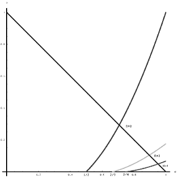
Figure 1: Parameter space $(d,b)$ of the phenotypic model with the critical curves $m=1$ for $R=2,3,4$.

Now we can make some quantitative predictions about the behaviour of the model.

One can localize in the parameter space $(b,d)$ each of the three regimes of the phenotypic model (sub-critical, super-critical, critical) by considering, for each fixed $R$, the critical curve $m(b,d,R)=1$ (see FIG. 1). The region of sub-criticality (for each fixed $R$) lies on the right side of the critical curve and the region of super-criticality (for each fixed $R$) lies on the left side of the critical curve.

Another interesting feature of the parameter space is related to the points of intersection of the critical curve $m(b,d,R)=1$ with the boundary curves $b+d=1$ and $b=0$. The points of intersection with the boundary curve $b=0$ are give by $d_{c}(R)=1-1/R$ and the points of intersection with the boundary curve $b+d=1$ have non-zero coordinates and can be written as $(1-b_{c},b_{c})$ where $b_{c}(R)$ is the $b$-coordinate and $1-b_{c}(R)$ is the $d$-coordinate. For instance, it is easy to find the exact value of $b_{c}$ for $R=2$: $b_{c}(2)=1-\tfrac{1}{\sqrt{2}}\cong 0.2928$. This calculation gives an important prediction: if $b>0.2929$ then the population can not become extinct by increasing $d$ towards its maximum value ($\cong 0.7070$), with probability going to $1$ as $R$ becomes large.

More generally, one has the following criterion of no sure extinction. Consider the phenotypic model with parameters $(b,d,R)$, with $R$ large enough. If $b\neq 0$ is sufficiently small and (up to order $\mathit{O}(b^{2})$)

$$b\,R(R-1)^{2}\geqslant 1$$ (9)

then, asymptotically almost surely, the population can not become extinct by increasing the deleterious probability towards its maximum value. In other words, when the inequality (9) is satisfied the process can have only one regime, namely, the supercritical, which renders the model completely trivial, since there is no transition.

This criterion follows from the approximation of $b_{c}(R)$ that can be obtained from the truncated perturbation expansion of the malthusian parameter. Solving the equation $m(b,1-b,R)=1$ for $b$ in terms of $R$ gives

$$b_{c}(R)\approx\dfrac{1}{R(R-1)^{2}}\,.$$ (10)

Here we should assume that $R$ is sufficiently large since the truncated expansion is a good approximation for $m$ only when $b$ is small. In fact, $R>10$ is reasonable, since $d_{c}(10)=0.9$ and $b_{c}(10)$ can be numerically evaluated to give $b_{c}(10)\cong 0.00486$. Using the approximation (10) one obtains $b_{c}(10)\approx 0.00123$.

From now on we shall split the analysis of the phenotypic model according to which it is sub-critical, super-critical or critical.

3.1 The Sub-critical Regime: Lethal Mutagenesis

The first consequence of our results is a proof, in the context of the phenotypic model (provided one assumes that all effects are of purely mutational nature), of the conjecture of lethal mutagenesis of Bull et al (2007). Recall that Bull et al (2007) assumes that all mutations are either neutral or deleterious and write the mutation rate $U=U_{d}+U_{c}$ where the component $U_{c}$ comprises the purely neutral mutations and the component $U_{d}$ comprises the mutations with a deleterious fitness effect. Let $R_{\mathrm{max}}$ denote the maximum reproductive capacity among all particles in the viral population. The extinction criterion proposed by Bull et al (2007) states that a sufficient condition for extinction is

$$\mathrm{e}^{-U_{d}}R_{\mathrm{max}}<1\,.$$ (11)

According to Bull et al (2007, 2008), $\mathrm{e}^{-U_{d}}$ is both the mean fitness level and also the fraction of offspring with no non-neutral mutations. In the absence of beneficial mutations the only type of non-neutral mutations are the deleterious mutations and hence $\mathrm{e}^{-U_{d}}=c=1-d$. Since the evolution of the mean values depends only on the expected values of the replication distribution $t_{r}$, it follows that $R_{\mathrm{max}}=R$. That is, the extinction criterion (11) is equivalent, in the context of the phenotypic model, to

$$(1-d)\,R<1\,,$$ (12)

which is exactly the condition for the model to be sub-critical. In Bull et al (2008) the authors suggest a modification of the extinction threshold (11) that accounts for beneficial effects as long as they do not couple the deleterious ones. Assuming that the population size is large enough and that a large number of individuals experience the full set of beneficial mutations they propose the following threshold

$$\mathrm{e}^{-U_{d}}\,R_{\mathrm{max}}\,(1+b)<1\,.$$ (13)

Our formula (8) for the malthusian parameter allows us to propose a generalization of the extinction threshold (11) without any extra assumptions: if $b\neq 0$ is sufficiently small (up to order $\mathit{O}(b^{2})$) and

$$(1-d)\,R\,\left(1+\dfrac{(R-1)\,d}{(1-d)^{2}}\,b\right)<1$$ (14)

then, with probability one, the population become extinct in finite time.

Observe that, when $b=0$ and $R$ fixed, the model becomes critical for $d=d_{c}(R)=1-1/R$. In other words, for every fixed mean replication capacity $R$, if the deleterious probability satisfies $d>d_{c}(R)$ then lethal mutagenesis occurs almost surely. Thus one may consider a general critical probability function $d_{c}(b,R)$ and in order to compute this probability as a function of $b$ and $R$ one must solve the equation $m(b,d,R)=1$ for $d$ in terms of $(b,R)$. This can be done by implicit differentiation of the equation $m(b,d,R)=1$:

$$\begin{split}d_{c}(b,R)&=(1-1/R)+b(R-1)^{2}+\mathit{O}(b^{2})\\ &=d_{c}(R)+b(R-1)^{2}+\mathit{O}(b^{2})\,.\end{split}$$ (15)

Formula (15) allows us to obtain a weak generalization of the extinction criterion to the case where $b$ is non-zero and $d\approx d_{c}(R)$. If $b\neq 0$ is sufficiently small and (up to order $\mathit{O}(b^{2})$)

$$(1-d)\,R<1-b\,R(R-1)^{2}$$ (16)

then, with probability one, the population become extinct in finite time. We summarize the discussion about extinction criteria in Table 1.

Extinction Criterion	Conditions	Comments
$(1-d)\,R<1$		The lethal mutagenesis criterion (LMC)
(no beneficial mutations)		of Bull et al (2007) with $(1-d)=\mathrm{e}^{-U_{d}}$
$(1-d)\,R\,(1+b)$	$b\approx 0$,	Generalization of the LMC proposed in
(uniform beneficial mutations)	$N\to\infty$	Bull et al (2008) ($N=$population size)
$(1-d)\,R\,\left(1+\dfrac{(R-1)\,d}{(1-d)^{2}}\,b\right)<1$	$b\approx 0$	Branching process generalization
(strong version)		obtained from perturbative expansion
$(1-d)\,R<1-b\,R(R-1)^{2}$	$b\approx 0$,	Branching process generalization
(weak version)	$d\approx d_{c}(R)$	solving implict equation $m(b,d,R)=1$

Table 1: Extinction criterion and its generaliations. The role of beneficial mutations $b$ in several forms.

The main conclusion here is that the existence of lethal mutagenesis depends on “genetic components” (mutational rates) and other additional deleterious effects (host driven pressures intensifications), as well as on strict “ecological components”, namely, the maximum replication capacity of the particles in the population and on the initial population size. As a result the viral population may reach extinction by increasing the number of deleterious mutations per replication cycle, by decreasing the value of $R$ in the population or by a combination of the two mechanisms. The mutational strategy is the basis of treatments using mutagenic drugs (see Crotty et al (2001)) that induce errors in the generation process of new viral particles reducing their replication capacity. A straightforward consequence of formulas (12), (14) and (16) is that a single particle showing the maximum replication capacity $R$ is able to rescue a viral population driven to extinction by mutagenic drugs. If it is assumed that RNA virus populations correspond to a swarm of variants with distinct replication capacities, for a therapy to become effective it is important that it will eliminate the classes represented by particles with highest replication capacities. In other words, the higher the replication capacity of the first particles infecting the organism the larger should be the number of deleterious mutations (or effects), that is, the larger should be the drug concentration. This can be a clear limitation for treatments based on mutagenic drugs.

3.2 The Super-critical Case: Relaxation and Equilibrium

In the super-critical regime, the population grows at a geometric pace indefinitely. Nevertheless, there are two distinct phases that occur during this growth: a transient phase (“relaxation”or “recovery time”) and a dynamical stationary phase.

3.2.1 Relaxation towards equilibrium

An important question concerning the adaptation process of a viral population to the host environment is the typical time needed to achieve the equilibrium state. As the equilibrium is characterized by constant mean replication capacity an obvious criteria to measure the time to achieve equilibrium would be by the vanishing of the variation of this variable as used in other studies (Aguirre et al, 2009). Nevertheless, this method is clearly subjected to the limitations of numerical accuracy with evident drawbacks if one wants a sharp and universal criterion to differentiate populations from the point of view of how fast a population can be typically stabilized in a organism.

Viral populations are commonly submitted to transient regimes. As pointed out earlier the infection transmission process represents the passage of a small number of particles from one organism to another in such a way that in this process the viral population is submitted to a subsequent bottle-neck effect during spreading of viruses in the host population. In order to approach the problem of relaxation after a bottleneck process in a more sound basis the natural quantity to be considered is the characteristic time derived from the decay of the mean auto-correlation function. When the temporal mean correlation function $C(n)$ is of the form $\exp(-n\alpha)$ the decay rate is defined as the parameter $\alpha$. The natural way to define the characteristic time $T$ to achieve equilibrium is by setting $T=1/\alpha$.

The temporal mean correlation function $C(n)$ may be calculated by considering recursive applications of the mean matrix $\bm{M}$ on the initial population: $\bm{Z}_{0}^{\mathrm{t}}\,\bm{M}^{n}\bm{Z}_{0}$. Since we are looking for bounds on the mean correlation function, it is enough to consider the canonical initial populations $\bm{Z}_{0}=\bm{e}_{r}$ and use the Perron-Frobenius theorem (see (Harris, 1963, p. 38) or (Athreya and Ney, 1972, p. 185)) to write

$$\bm{Z}_{0}^{\mathrm{t}}\,\bm{M}^{n}\bm{Z}_{0}=m^{n}\big{(}u_{R}(r)v_{R}(r)\big{)}+\mathit{O}(\varrho_{0}^{n})\,,$$

where $\bm{u}_{R}$ is the normalized right eigenvector and $\bm{v}_{R}$ is normalized left eigenvector (see the appendix for more details) corresponding to $m$ and $0<\varrho_{0}<m$. Moreover, since we are assuming that $m>1$, it follows that $0<\tfrac{\mathit{O}(\varrho_{0}^{n})}{m^{n}}<1$ and $\tfrac{\mathit{O}(\varrho_{0}^{n})}{m^{n}}\to 0$ as $n$ goes to infinity.

Define the type $r$ of an initial population $\bm{Z}_{0}$ as the largest replicative class $r$ represented in that population. In general, the mean correlation function will depend only on the type $r$ of the initial population and will be denoted by $C_{r}(n)$. Therefore, the mean correlation function is typically exponential and given by

$$C_{r}(n)=K_{r}(n)\exp\big{(}-n\log(m)\big{)}\,,$$

where $K_{r}(n)$ ($r=0,\ldots,R)$ is given by

$$K_{r}(n)=\dfrac{1}{\bm{u}_{R}(r)\bm{v}_{R}(r)+\tfrac{\mathit{O}(\varrho_{0}^{n})}{m^{n}}}\,.$$

It is difficult, in general, to calculate an explicit expression of $\bm{u}_{R}(r)\bm{v}_{R}(r)$, but it is easy to see that

$$\dfrac{1}{1+\bm{u}_{R}(r)\bm{v}_{R}(r)}<K_{r}(n)<\dfrac{1}{\bm{u}_{R}(r)\bm{v}_{R}(r)}$$

and so the time dependence of $K_{r}$ is negligible. Indeed, for $n$ sufficiently large the dominating factor of $C_{r}(n)$ is the exponential.

The lower bound for the mean correlation is attained when the type of the initial population is $R$, that is,

$$K_{R}\approx 1+\mathit{O}(b)\approx 1\,.$$

In this case the mean correlation function is

$$C_{R}(n)\approx\exp\big{(}-n\log(m)\big{)}\,,$$

very similar to the case with no beneficial effects. In fact, in this particular case $b=0$ and one has $K_{r}=1$, for every $r$, so it is enough to consider the case $\bm{Z}_{0}=\bm{e}_{R}$, that is,

$$C(n)=\exp(-n\log(R(1-d)))\,.$$

The difference between these two cases lies on the value of the largest eigenvalue (the correlation decay rate) $m$. As $m(b)>m(0)$ for the same values of $d$ and $R$ the correlation function decays faster if beneficial effects are present.

In general, we have that (see the appendix)

$$K_{r}\approx\mathit{O}(b^{-(R-r)})\qquad\text{for}\quad r=1,\ldots,R\,.$$

Hence the mean correlation function may be written as

$$C_{r}(n)\approx\dfrac{\kappa_{r}}{b^{R-r}}\,\exp\big{(}-n\log(m)\big{)}\,,$$

where $\kappa_{r}=\kappa_{r}(d,R)$.

The conclusion here is that when the type of the initial population is $r$ there is a “delay effect” on the decay of the mean correlation of order $b^{-(R-r)}$ relative to the fastest decay (lower bound) $C_{R}(n)$. The slowest possible decay (upper bound) is attained when the type of the population is $r=1$, which have a delay of order $b^{-(R-1)}$. This “delay effect” on the mean correlation appears in simulations as “jumps” of magnitude $(1-d)$ of the mean replicative capacity, somewhat reminiscent of the “punctuated equilibrium scenario”.

Observe that the closer is the parameter $d$ to its critical value $d_{c}$, the longer is the time needed to achieve equilibrium. The clearest way to characterize the time behavior of the viral population at or around the critical point is through the typical time $T$ to approach equilibrium derived from the decay of correlations described above. The expression $T=1/\log(m)$ shows that at the critical point the equilibrium state is never reached, i.e., the decay to equilibrium is at least non-exponential. A scaling exponent characterizing the behavior of $T$ in the neighborhood of the critical point $d_{c}$ can be easily obtained. The expansion around $d_{c}$ gives

$$T\approx|m-1|^{-1}=\dfrac{1}{m^{\prime}(d_{c})}\,|d-d_{c}|^{-1}\,.$$

In the particular case where $b=0$ we have

$$T\approx(1-d_{c})\,|d-d_{c}|^{-1}\,,$$

and hence $1/m^{\prime}(d_{c})=(1-d_{c})+\mathit{O}(b)$.

One possible application of this result relates to the very initial phase of the infection process. If one considers that during this phase the host immune system has not been yet stimulated against the virus, one can assume that the deleterious effects would be solely represented by the viral intrinsic mutation rates. Therefore, the largest the value of $R$, i.e., the largest the replication capacity of the initial viral particle, the fastest the decay of the progeny auto-correlation. Intuitively the parameter $R$ defines the degree of virulence of the infection during the early stage of the infective process.

3.2.2 The Dynamical Stationary State

According to the “Malthusian Law of Growth” it is expected that a super-critical branching process will grow indefinitely at a geometric rate proportional to $m^{n}$, that is, $\bm{Z}_{n}\approx m^{n}\,\bm{W}_{n}$, where $\bm{W}_{n}$ is a random vector. That is, the normalized random vector $\bm{W}_{n}=\bm{Z}_{n}/m^{n}$ posses a finite limit when $n\to\infty$. More precisely, there exists a random variable $\bm{W}\neq 0$ such that, with probability $1$,

$$\lim_{n\to\infty}\bm{W}_{n}=\bm{W}\,.$$

Moreover, $\bm{W}=W\bm{u}$ where $\bm{u}$ is the normalized right eigenvector corresponding to the malthusian parameter $m$ and

$$\mathbf{E}(W|\bm{Z}_{0})=\langle\bm{v},\bm{Z}_{0}\rangle\,,$$

where $\bm{v}$ is the left eigenvector corresponding to the malthusian parameter $m$. The meaning of this result is that the total size of the population divided by $m^{n}$, converges to a random vector, but the relative frequencies of the classes of particles approach fixed limits. In fact, (Kurtz et al, 1994) formalized this statement as a limit theorem (no averages here!):

$$\lim_{n\to\infty}\,\dfrac{\bm{Z}_{n}}{|\bm{Z}_{n}|}=\bm{u}\qquad\text{(almost surely).}$$ (17)

This result is useful in computational simulations of the model, since one may find an approximation to the “deterministic part” of $\bm{W}$ by sampling the population and computing the relative frequencies of replicative classes.

Recall that the normalized right eigenvector $\bm{u}_{R}=(u_{R}(0),\ldots,u_{R}(R))$ corresponding to the malthusian parameter $m$ is positive and is normalized so that $\sum_{r}u_{R}(r)=1$, therefore, it may be seen as a probability distribution on the set of classes $\{0,\ldots,R\}$. It is called the mean fitness distribution of the replicative classes of the viral population.

Using the same perturbative techniques as before, it is possible to compute the perturbation expansion of the right eigenvector corresponding to the malthusian parameter. We are interested in the right eigenvector $\bm{u}_{R}$ associated to the malthusian parameter $m$. The first order expansion of the normalized right eigenvector $\bm{u}_{R}$ associated to $m$ may be written as

$$\bm{u}_{R}=\bm{u}_{R}^{0}+b\,\sum_{k=0}^{R}\beta_{k}\bm{u}_{k}^{0}+\mathit{O}(b^{2})\,,$$ (18)

where the terms $\beta_{k}$ are functions of $d$ and $R$. The explicit expressions of the terms $\beta_{k}$ are somewhat cumbersome, however we still can use the abstract formula to gain some insight about $\bm{u}_{R}$.

The normalized right eigenvector $\bm{u}_{R}^{0}$ of $\bm{M}_{0}$ is

$$\bm{u}_{R}^{0}(r)=\mathrm{binom}(r;R,1-d)=\tbinom{R}{r}\,(1-d)^{r}\,d^{R-r}\,.$$

From these formulas one immediately obtains, for $b=0$:

• The mean replication capacity $\mathbf{E}(\bm{u}_{R}^{0})=R(1-d)$.

• The phenotypic diversity $\mathbf{Var}(\bm{u}_{R}^{0})=Rd(1-d)$.

In general, the mean replication capacity of a viral population is given by

$$\mathbf{E}(\bm{u}_{R})=\sum_{k=0}^{R}k\,u_{R}(k)=m\,.$$ (19)

Indeed, the malthusian parameter may be calculated as

$$m=\lim_{n\to\infty}\dfrac{|\langle\bm{Z}_{n+1}\rangle|}{|\langle\bm{Z}_{n}\rangle|}=\lim_{n\to\infty}\dfrac{|\bm{M}\langle\bm{Z}_{n}\rangle|}{|\langle\bm{Z}_{n}\rangle|}\,.$$

Now it is easy to see that $|\bm{M}\langle\bm{Z}_{n}\rangle|=\sum_{k}kZ_{n}^{k}$ and hence by the Perron-Frobenius theorem, equation (19) follows immediately. In particular, when $b\neq 0$ is small enough:

$$\mathbf{E}(\bm{u}_{R})=R(1-d)+\dfrac{(R-1)\,d}{1-d}\,R\,b+\mathit{O}(b^{2})\,.$$

Using (18) one may write the phenotypic diversity of a viral population as:

$$\mathbf{Var}(\bm{u}_{R})=Rd(1-d)+\left(2\sum_{k=0}^{R}\beta_{k}\,\mathbf{Cov}(\bm{u}_{R}^{0},\bm{u}_{k}^{0})\right)\,b+\mathit{O}(b^{2})\,.$$ (20)

It is possible to estimate the magnitude of the first order perturbation term in eq. (20):

$$\mathbf{Var}(\bm{u}_{R})\approx Rd(1-d)\bigg{(}1+8b\dfrac{R-1}{R}\dfrac{dR-1+(1-d)^{R}}{d^{2}}\bigg{)}.$$

It is well accepted that the phenotypic diversity is an important characteristic of the viral population intuitively related to the idea of population robustness (Forster et al, 2006; Elena et al, 2007). In fact, a homogeneous population would be less flexible from the point of view of adaptation. The variance associated with the stationary state can be seen as a measure of phenotypic diversity. It shows that, in the case where $b=0$, the maximum value of the phenotypic diversity $R/4$ is reached if $d=1/2$ for any value of $R$. For $b\neq 0$ it can be shown numerically, that there is always a value $d_{\mathrm{max}}$ of $d$ for which the population attains maximal phenotypic diversity. This value $d_{\mathrm{max}}$ is a decreasing function of $b$. For $b\approx 0$ this value is $d_{\mathrm{max}}\lesssim 1/2$.

It is interesting to note that experimental measurements of $c=1-d$ are close to $0.5$ (Sanjuán et al, 2004; Domingo-Calap et al, 2009), suggesting that viral populations follow a principle of maximal phenotypic diversity.

As far as the experimental situation of the phenotypic diversity is concerned, one of the first attempts to experimentally measure the phenotypic diversity was in Delbrück (1945), where the total “burst size” of a progeny from phage-infected bacterial cells was estimated. More recently, measurements of the phenotypic diversity in vitro generated by single viral particles infecting individual cells (Zhu et al, 2009; Timm and Yin, 2012) revealed a broad distribution of virus yields ($50$ to $8000$ progeny virus particles). One may regard these results as indication that the replicative capacity of a virus from a particular replicative class is characterized by a fitness distribution obtained as the distribution of progeny produced by representative particles from that same replicative class. Although these authors did not went further and investigated if different particles form a viral population have different fitness distributions their results suggest that a fitness distribution over a viral population may resemble the mean fitness distribution of the replicative classes obtained from the phenotypic model. In this direction, further carefully designed experiments aiming at determine the mean fitness distribution of a viral population would be welcome.

3.3 Criticality and Eigen’s Error Threshold

The relation between multitype branching processes and Eigen’s theory of evolution of macromolecules (Eigen, 1971) has been established by Demetrius et al (1985). In this work it is shown that one may canonically associate a certain difference equation to a discrete time multitype branching process through its mean matrix. This deterministic dynamical system is called Eigen’s selection equation, due to its similarity to the phenomenological equation describing the kinetics of self-reproducing molecules in a dialysis reactor. Moreover, the selection equation is essentially equivalent to a linear difference equation $\bm{x}_{n}=\bm{M}^{n}\bm{x}_{0}$, where $\bm{M}$ is the mean matrix of the branching process. Note that this equation is formally identical to the equation for the evolution of the mean values of branching process (see eq. (3)). Hence the selection equation may be seen as a mean field limit equation associated branching process. In particular, when the process does not become extinct, part of its asymptotic behaviour, namely, the relative frequencies the classes, can be recovered by the selection equation. Moreover, it is shown that a super-critical branching process displays “freezing in” of initial fluctuations, that is, the coefficient of variation of the process vanishes asymptotically almost sure. In this sense, if the population is infinite and one waits long enough before starting observation, the deterministic model is fairly reliable because fluctuations are small. Nonetheless, when considering finite populations, i.e., finite size samples of each generation, the deterministic approximation is only part of the story, since the fluctuations contain the “out-of-equilibrium” characteristics of the system.

The use of branching processes links the concept of error threshold with that of criticality. If we switch to the genotypic view of Demetrius et al (1985) and suppose that there are no back-mutations ($b=0$) then we can consider polymers with chain length of $\nu$ nucleotides and that there is a fixed probability $p$ for copying a single nucleotide correctly, that is, $c=p^{\nu}$. The formula for the malthusian parameter ($m=cR=p^{\nu}R$) together with the criticality condition ($m=1$) gives the stochastic error threshold of (Demetrius et al, 1985, p. 254, eq. (47)):

$$\nu_{\mathrm{s}}~{}=~{}\dfrac{\;\ln R}{-\ln p}\,.$$ (21)

Since the lethal mutagenesis criterion, in the context of branching processes, is exactly the criticality condition, the stochastic error threshold refers to the probability of extinction. This can be compared with the deterministic error threshold (see Eigen (1971); Eigen and Schuster (1979); Swetina and Schuster (1982)):

$$\nu_{\mathrm{d}}~{}=~{}\dfrac{\;\ln\sigma}{-\ln p}\,,$$ (22)

where the parameter $\sigma$ is the superiority of the master sequence (see Demetrius et al (1985)). The deterministic error threshold is based on the condition that the error-free productivity of the master molecular species becomes equal to the mean total productivity of all other species. The condition to replicate with a fidelity above the error threshold will always be valid for the master species provided the mutation terms of all other species are sufficiently small. Beyond that point, the master species is no longer maintained: the population has reached the error catastrophe (Bull et al, 2005). Moreover, the demand to operate above the stochastic threshold is always a stronger condition than the corresponding requirement of the deterministic equation.

It is interesting to note that at the critical point the dynamics of the branching process relax to equilibrium according to the typical algebraic decay in time. This property raises the question (unapproachable in the present context) if the classes in the critical population are so strongly correlated in such a way that the whole population behaves as if it is composed be only one replicative class. This behaviour reminds one of the basic properties of the error threshold in Eigen’s theory of macromolecular evolution (Eigen, 1971).

Preliminary results concerning the dynamics of fluctuations (Antoneli et al (2013b); Castro (2011)) indeed show that the time variation of the numbers of particles in each separated class follows a pattern such that the variation observed in one class is rigorously the same observed in all the others. This indicate a high level of correlation between the classes in complete analogy with critical phenomena of many physical systems. It is worth to note that, in fact, there is a correspondence between Eigen’s model and the equilibrium statistical mechanics of a certain inhomogeneous Ising system (see Leuthäusser (1987)).

4 Outlook

Modeling the dynamics of viral populations by means of multivariate branching processes does not take into account many molecular/microscopic details of the replicative process, nevertheless, it is remarkable that the provided description at the population/macroscopic scale is very appealing and well fitted to various aspects of the observed phenomenology of viral systems. This leads to the conclusion that we are probably far from exhaust the analytical and predictive power of branching processes as a mathematical tool for the study of viral populations. In fact, many aspects of the problem like (i) the role of finite size effects, (ii) the role of different infected cell types for the problem of evolution of viral populations in multi-cellular hosts, (iii) the relation between quiescent infected cells with branching process with singular components and (iv) the descriptive limits of discrete versus continuous time branching processes, are still to be considered by future investigations. Also it is worth to mention that most of the quantitative results and all of the qualitative observations described here can be easily reproduced by computer simulation of the model (see Castro Castro (2011) and manuscript in preparation Castro et al (2011)).

Finally, it is important to emphasize that the branching process analysis carried out here revolves around the malthusian parameter, which is based on certain critical assumptions regarding environmental constraints, for instance, that the environment (host) does not change dramatically. The significance of this macroscopic measure in studies of evolutionary processes has been challenged in a series of articles (see Dietz (2005); Kowald and Demetrius (2005); Ziehe and Demetrius (2005)). When the environment is strongly perturbed, another parameters become important, as the “evolutionary entropy”, which is a measure of the variability in the age at which individuals produce offspring and die (see Kowald and Demetrius (2005); Ziehe and Demetrius (2005)). These parameters will play a role in studies of the extinction process.

Appendix: Spectral Perturbation Theory

In order to carry out the perturbative calculations we need to solve the spectral problem for the matrix

$$\bm{M}_{0}=\begin{pmatrix}0&d&0&\ldots&0\\ 0&(1-d)&2d&\ldots&0\\ 0&0&2(1-d)&\ldots&0\\ 0&0&0&\ldots&0\\[-5.69054pt] \vdots&\vdots&\vdots&\ddots&Rd\\ 0&0&0&\ldots&R(1-d)\end{pmatrix}\,.$$

The eigenvalues $\lambda_{r}^{0}$ of the mean matrix $\bm{M}_{0}$ are:

$$\lambda_{r}^{0}=rc=r(1-d)\qquad r=0,\ldots,R\,.$$

In particular, the malthusian parameter is the largest positive eigenvalue

$$m^{0}=\lambda_{R}^{0}=Rc=R(1-d)\,.$$

The normalized left and right eigenvectors, $\bm{v}_{r}^{0}$ and $\bm{u}_{r}^{0}$, associated to the eigenvalue $\lambda_{r}^{0}$, satisfy:

$$(\bm{v}_{s}^{0})^{\mathrm{t}}\bm{u}_{s}^{0}=1\quad\text{and}\quad\bm{1}^{\mathrm{t}}\bm{u}_{s}^{0}=1\,.$$

Writing $\bm{v}_{r}^{0}$ and $\bm{u}_{r}^{0}$ in components as

$$\begin{split}\bm{v}_{r}^{0}&=\big{(}v_{r}^{0}(0),v_{r}^{0}(1),\ldots,v_{r}^{0}(R)\big{)}\,,\\ \bm{u}_{r}^{0}&=\big{(}u_{r}^{0}(0),u_{r}^{0}(1),\ldots,u_{r}^{0}(R)\big{)}\,,\end{split}$$

one has that

$$v_{r}^{0}(k)=\left\{\begin{array}[]{c@{\quad\text{for}\quad}c}0&k=0,\ldots,r-1\,,\\[8.53581pt] \dfrac{-d(r+1)}{(1-d)^{r+1}}&k=r+1\\[8.53581pt] \dfrac{((-1)\,d)^{k-r}}{(1-d)^{k}}&k=r,r+2,\ldots,R\,.\end{array}\right.$$

and

$$u_{r}^{0}(k)=\left\{\begin{array}[]{c@{\quad\text{for}\quad}c}\tbinom{r}{k}\,(1-d)^{k}\,d^{r-k}&k=0,\ldots,r\,,\\[5.69054pt] 0&k=r+1,\ldots,R\,.\end{array}\right.$$

Now we write the eigenvalue $\lambda_{r}$ of $\bm{M}$ as a function of the parameter $b$, expanded as a power series

$$\lambda_{r}=\lambda_{r}^{0}+\lambda_{r}^{1}b+\lambda_{r}^{2}b^{2}+\ldots\,,$$

where $\lambda_{r}^{0}$ is the corresponding eigenvalue of $\bm{M}_{0}$. Clearly, $\lambda_{r}(b)\to\lambda_{r}^{0}$ as $b\to 0$. The higher order perturbation coefficients $\lambda_{r}^{i}$, ($i=1,2,3,\ldots$) are written in terms of all the eigenvalues $\lambda_{s}^{0}$ ($s=0,\ldots,R$) of $\bm{M}_{0}$ and their associated left and right normalized eigenvectors $\bm{v}_{s}^{0}$ and $\bm{u}_{s}^{0}$ and the perturbation matrix

$$\bm{P}=\begin{pmatrix}0&0&0&0&0&\ldots&0&0\\ 0&-1&0&0&0&\ldots&0&0\\ 0&1&-2&0&0&\ldots&0&0\\ 0&0&2&-3&0&\ldots&0&0\\ 0&0&0&3&-4&\ldots&0&0\\[-5.69054pt] \vdots&\vdots&\vdots&\vdots&\vdots&\ddots&\vdots&\vdots\\ 0&0&0&0&0&\ldots&-(R-1)&0\\ 0&0&0&0&0&\ldots&(R-1)&0\end{pmatrix}\,.$$

Note that the operator norm of $\bm{P}$ is $\|\bm{P}\|=2(R-1)$ and so the magnitude of the perturbation is $2b(R-1)$.

The general expressions for the first and second order coefficients of the perturbation expansion of an eigenvalue are

$$\begin{split}\lambda_{r}^{1}&=(\bm{v}_{r}^{0})^{\mathrm{t}}\bm{P}\bm{u}_{r}^{0}\,,\\ \lambda_{r}^{2}&=\sum_{s\neq r}\dfrac{\big{[}(\bm{v}_{s}^{0})^{\mathrm{t}}\bm{P}\bm{u}_{r}^{0}\big{]}\,\big{[}(\bm{v}_{r}^{0})^{\mathrm{t}}\bm{P}\bm{u}_{s}^{0}\big{]}}{\lambda_{r}^{0}-\lambda_{i}^{0}}\,.\end{split}$$

We want to use these formulas to compute a perturbation approximation (for $b$ around $0$) of the malthusian parameter $m(b)$ of $\bm{(}M)$. Recall that, $m(0)=m^{0}=R(1-d)$ and the corresponding left and right eigenvectors are given by

$$\begin{split}\bm{v}_{R}^{0}&=1/(1-d)^{R}(0,\ldots,0,1)\,,\\ \bm{u}_{R}^{0}&=(u_{R}(0),\ldots,u_{R}(R))\,,\end{split}$$

with $u_{R}(k)=\mathrm{binom}(k;R,1-d)$. The first order coefficient of the malthusian parameter is

$$m^{1}=(\bm{v}_{R}^{0})^{\mathrm{t}}\bm{P}\bm{u}_{R}^{0}=\dfrac{(R-1)u_{R}(R-1)}{(1-d)^{R}}=\dfrac{R(R-1)d}{1-d}\,.$$

For the second order coefficient we also need

$$\bm{v}_{R-1}^{0}=1/(1-d)^{R-1}(0,\ldots,0,1,-Rd/(1-d))\,.$$

The second order coefficient is

$$\begin{split}m^{2}&=\sum_{i=0}^{R-1}\dfrac{\big{[}(\bm{v}_{i}^{0})^{\mathrm{t}}\bm{P}\bm{u}_{R}^{0}\big{]}\,\big{[}(\bm{v}_{R}^{0})^{\mathrm{t}}\bm{P}\bm{u}_{i}^{0}\big{]}}{\lambda_{R}^{0}-\lambda_{i}^{0}}\\[8.53581pt] &=\dfrac{\big{[}(\bm{v}_{R-1}^{0})^{\mathrm{t}}\bm{P}\bm{u}_{R}^{0}\big{]}\,\big{[}(\bm{v}_{R}^{0})^{\mathrm{t}}\bm{P}\bm{u}_{R-1}^{0}\big{]}}{(1-d)}\\[8.53581pt] &=-\dfrac{R(R-1)^{2}(1+\tfrac{R}{2}\,d)d}{(1-d)^{3}}\,.\end{split}$$

Analogous perturbative formulas exist for the perturbation expansion of the left and right eigenvector corresponding to an eigenvalue $\lambda_{r}$. The left and right eigenvector $\bm{v}_{r}$ and $\bm{u}_{r}$ of the matrix $\bm{M}$ associated with the eigenvalue $\lambda_{r}$ can be written as a function of the parameter $b$, expanded as a vector-valued power series:

$$\begin{split}\bm{v}_{r}&=\bm{v}_{r}^{0}+b\,\sum_{s\neq r}A_{r,s}^{1}\bm{v}_{s}^{0}+b^{2}\,\sum_{s\neq r}A_{r,s}^{2}\bm{v}_{s}^{0}+\ldots\,,\\ \bm{u}_{r}&=\bm{u}_{r}^{0}+b\,\sum_{s\neq r}B_{r,s}^{1}\bm{u}_{s}^{0}+b^{2}\,\sum_{s\neq r}B_{r,s}^{2}\bm{u}_{s}^{0}+\ldots\,,\end{split}$$

where $\bm{v}_{r}^{0}$ and $\bm{u}_{r}^{0}$ are, respectively, the left and right eigenvectors of the matrix $\bm{M}_{0}$ associated to the eigenvalue $\lambda_{r}^{0}$. The perturbation terms $A_{r,s}^{i}$ and $B_{r,s}^{i}$ with $i=1,2,3,\ldots\,$, can be written in terms of the eigenvalues of $\bm{M}_{0}$ and their associated left and right eigenvectors and the perturbation matrix $\bm{P}$. Observe that when $b\to 0$ we get the normalized left and right eigenvectors $\bm{v}_{R}^{0}$ and $\bm{u}_{R}^{0}$ associated to the dominant eigenvalue $m^{0}=(1-d)R$ of the mean matrix $\bm{M}_{0}$.

We are interested in the normalized eigenvectors $\bm{v}_{R}$ and $\bm{u}_{R}$ associated to the malthusian parameter $m=(1-d)R$

$$\bm{v}_{R}=\bm{v}_{R}^{0}+b\,\sum_{k=0}^{R}\alpha_{k}\bm{v}_{k}^{0}+\mathit{O}(b^{2})\,,$$

with $\alpha_{k}=A_{R,k}^{1}$, ($0\leqslant k\leqslant R-1$) and $\alpha_{R}=-\sum_{k=0}^{R-1}\alpha_{k}$,

$$\bm{u}_{R}=\bm{u}_{R}^{0}+b\,\sum_{k=0}^{R}\beta_{k}\bm{u}_{k}^{0}+\mathit{O}(b^{2})\,,$$

with $\beta_{k}=B_{R,k}^{1}$, ($0\leqslant k\leqslant R-1$) and $\beta_{R}=-\sum_{k=0}^{R-1}\beta_{k}$.

The first order coefficients are given by

$$\begin{split}A_{R,s}^{1}&=\dfrac{(\bm{v}_{R}^{0})^{\mathrm{t}}\bm{P}\bm{u}_{s}^{0}}{\lambda_{R}^{0}-\lambda_{s}^{0}}\,,\\ B_{R,s}^{1}&=\dfrac{(\bm{v}_{s}^{0})^{\mathrm{t}}\bm{P}\bm{u}_{R}^{0}}{\lambda_{R}^{0}-\lambda_{s}^{0}}\,,\end{split}$$

and the second order terms are given by

$$\begin{split}A_{R,s}^{2}&=\sum_{i=0}^{R-1}\dfrac{\big{[}(\bm{v}_{R}^{0})^{\mathrm{t}}\bm{P}\bm{u}_{i}^{0}\big{]}\,\big{[}(\bm{v}_{i}^{0})^{\mathrm{t}}\bm{P}\bm{u}_{s}^{0}\big{]}}{(\lambda_{R}^{0}-\lambda_{s}^{0})\,(\lambda_{R}^{0}-\lambda_{i}^{0})}\,,\\ B_{R,s}^{2}&=\sum_{i=0}^{R-1}\dfrac{\big{[}(\bm{v}_{s}^{0})^{\mathrm{t}}\bm{P}\bm{u}_{i}^{0}\big{]}\,\big{[}(\bm{v}_{i}^{0})^{\mathrm{t}}\bm{P}\bm{u}_{R}^{0}\big{]}}{(\lambda_{R}^{0}-\lambda_{s}^{0})\,(\lambda_{R}^{0}-\lambda_{i}^{0})}\,,\end{split}$$

for $s=0,\ldots,R-1$.

One may use the formula of $\bm{v}_{R}$ up to second order

$$\bm{v}_{R}=\bm{v}_{R}^{0}+b\,\dfrac{(R-1)}{(1-d)^{2}}\,\bm{v}_{R-1}^{0}+\mathit{O}(b^{2})$$

and the first order expansion $\bm{u}_{R}=\bm{u}_{R}^{0}+\mathit{O}(b)$ in order to estimate the product of coefficients $u_{R}(r)v_{R}(r)$ (up to their leading order). For instance, it is easy to find that

$$\begin{split}u_{R}(R)v_{R}(R)=1+\mathit{O}(b)&=\mathit{O}(1)\,,\\ u_{R}(R-1)v_{R}(R-1)&=\mathit{O}(b)\,,\\ u_{R}(R-2)v_{R}(R-2)&=\mathit{O}(b^{2})\,.\end{split}$$

In general, using a higher order expansion formula for $\bm{v}_{R}$, one concludes that

$$u_{R}(R-r)v_{R}(R-r)=\mathit{O}(b^{r})\,.$$

This follows form the fact that the coefficient of order $b^{r}$ in the perturbation expansion of $\bm{v}_{R}$ is a linear combination of the left eigenvectors $\bm{v}_{R-1}^{0},\ldots,\bm{v}_{r-R}^{0}$, all of which have zeros in the first $r-1$ components.

References

- Aguirre and Manrubia (2008) Aguirre J, Manrubia SC (2008) Effects of spatial competition on the diversity of a quasispecies. Phys Rev Lett 100(3):038,106
- Aguirre et al (2009) Aguirre J, Lázaro E, Manrubia SC (2009) A trade-off between neutrality and adaptability limits the optimization of viral quasispecies. J Theor Biol 261:148–155
- Antoneli et al (2005) Antoneli F, Dias APS, Golubitsky M, Wang Y (2005) Patterns of synchrony in lattice dynamical systems. Nonlinearity 18(5):2193–2209, DOI 10.1088/0951-7715/18/5/016
- Antoneli et al (2013a) Antoneli F, Bosco F, Castro D, Janini LM (2013a) Viral evolution and adaptation as a multivariate branching process. In: Mondaini RP (ed) BIOMAT 2012 – Proceedings of the International Symposium on Mathematical and Computational Biology, World Scientific, URL http://arxiv.org/abs/1110.3368
- Antoneli et al (2013b) Antoneli F, Bosco F, Janini LM (2013b) Fluctuations and correlations in a viral quasi-species. In preparation
- Athreya and Ney (1972) Athreya KB, Ney PE (1972) Branching Processes. Springer-Verlag, Berlin
- Bull et al (2005) Bull JJ, Meyers LA, Lachmann M (2005) Quasispecies made simple. PLoS Comp Biol 1(6):450–460
- Bull et al (2007) Bull JJ, Sanjuán R, Wilke CO (2007) Theory of lethal mutagenesis for viruses. J Virology 18(6):2930–2939, DOI doi:10.1128/JVI.01624-06
- Bull et al (2008) Bull JJ, Sanjuán R, Wilke CO (2008) Lethal mutagenesis. In: Domingo E, Parrish CR, Holland JJ (eds) Origin and Evolution of Viruses, second edition edn, Academic Press, London, chap 9, pp 207–218, DOI 10.1016/B978-0-12-374153-0.00009-6
- Capitán et al (2011) Capitán JA, Cuesta JA, Manrubia SC, Aguirre J (2011) Severe hindrance of viral infection propagation in spatially extended hosts. PLoS One 6(8):e23,358, DOI 10.1371/journal.pone.0023358
- Carrasco et al (2007) Carrasco P, de la Iglesia F, Elena SF (2007) Distribution of fitness and virulence effects caused by single-nucleotide substitutions in Tobacco Etch Virus. J Virology 18(23):12,979–12,984
- Castro (2011) Castro D (2011) Simulação computacional e análise de um modelo fenotípico de evolução viral. Master’s thesis, Universidade Federal de São Paulo - UNIFESP, São Paulo
- Castro et al (2011) Castro D, Antoneli F, Bosco F, Janini LM (2011) Computational simulation of a model for viral evolution. In preparation 0:0
- Crotty et al (2001) Crotty S, Cameron CE, Andino R (2001) RNA virus error catastrophe: direct molecular test by using ribavirin. Proc Natl Acad Sci U S A 98:6895–6900
- Cuesta (2011) Cuesta JA (2011) Huge progeny production during transient of a quasi-species model of viral infection, reproduction and mutation. Math Comp Model 54:1676–1681
- Cuesta et al (2011) Cuesta JA, Aguirre J, Capitán JA, Manrubia SC (2011) Struggle for space: viral extinction through competition for cells. Phys Rev Lett 106(2):028,104–028,104
- Delbrück (1945) Delbrück M (1945) The burst size distribution in the growth of bacterial viruses (bacteriophages). J Bacteriol 50(2):131–135
- Demetrius et al (1985) Demetrius L, Schuster P, Sigmund K (1985) Polynucleotide evolution and branching processes. Bull Math Biol 47(2):239–262, URL http://www.springerlink.com/content/h362q6007842h042/
- Dietz (2005) Dietz K (2005) Darwinian fitness, evolutionary entropy and directionality theory. BioEssays 27:1097–1101
- Domingo and et al. (1985) Domingo E, et al (1985) The quasispecies (extremely heterogeneous) nature of viral rna genome populations: biological relevance – a review. Gene 40(1):1–8
- Domingo et al (1998) Domingo E, Baranowski E, Ruiz-Jarabo CM, Martín-Hernández AM, Sáiz JC, Escarmís C (1998) Quasispecies structure and persistence of rna viruses. Emerg Infect Dis 4(4):521–527
- Domingo-Calap et al (2009) Domingo-Calap P, Cuevas JM, Sanjuán R (2009) The fitness effects of random mutations in single-stranded DNA and RNA bacteriophages. PLoS Genet 5(11):e1000,742
- Eigen (1971) Eigen M (1971) Selforganization of matter and the evolution of biological macromolecules. Naturwissenschaften 58:465–523
- Eigen and Schuster (1979) Eigen M, Schuster P (1979) The Hypercycle. A principle of natural self-organization. Springer-Verlag, Berlin
- Elena and Sanjuán (2005) Elena SF, Sanjuán R (2005) Adaptive value of high mutation rates of rna viruses: separating causes from consequences. J Virology 79(18):11,555–11,558, DOI 10.1128/JVI.79.18.11555-11558.2005
- Elena et al (2007) Elena SF, Wilke CO, Ofria C, Lenski RE (2007) Effects of population size and mutation rate on the evolution of mutational robustness. Evolution 61(3):666–674, DOI 10.1111/j.1558-5646.2007.00064.x
- Escarmís et al (2006) Escarmís C, Lázaro E, Manrubia SC (2006) Population bottlenecks in quasispecies dynamics. Curr Top Microbiol Immunol 299:141–170
- Eyre-Walker and Keightley (2007) Eyre-Walker A, Keightley PD (2007) The distribution of fitness effects of new mutations. Nat Rev Genet 8(8):610–618, DOI 10.1038/nrg2146
- Feller (1968) Feller W (1968) An Introduction to Probability Theory and Its Applications, vol 1, 3rd edn. Wiley, New York
- Forster et al (2006) Forster R, Adami C, Wilke CO (2006) Selection for mutational robustness in finite populations. J Theor Biol 243(2):181–190, DOI 10.1016/j.jtbi.2006.06.020
- Gantmacher (2005) Gantmacher F (2005) Applications of the Theory of Matrices. Dover Publications, New York
- Gray (2006) Gray RM (2006) Toeplitz and Circulant Matrices: A review. Now Publishers Inc.
- Grenander and Szegö (1958) Grenander U, Szegö G (1958) Toeplitz Forms and Their Applications. University of California Press
- Harris (1963) Harris T (1963) The Theory of Branching Processes. Springer-Verlag, Berlin
- Hermisson et al (2002) Hermisson J, Redner O, Wagner H, Baake E (2002) Mutation-selection balance: ancestry, load, and maximum principle. Theor Popul Biol 62(1):9–46, DOI 10.1006/tpbi.2002.1582
- Imhof and Schlotterer (2001) Imhof M, Schlotterer C (2001) Fitness effects of advantageous mutations in evolving escherichia coli populations. Proc Natl Acad Sci U S A 98(3):1113–1117, DOI 10.1073/pnas.98.3.1113
- Jagers et al (2007) Jagers P, Klebaner FC, Sagitov S (2007) On the path to extinction. Proc Natl Acad Sci U S A 104(15):6107–6111
- Jiřina (1970) Jiřina M (1970) A simplified proof of the Sevastyanov theorem on branching processes. Annales de l’I H Poincaré, Section B 6(1):1–7
- Keightley and Lynch (2003) Keightley PD, Lynch M (2003) Toward a realistic model of mutations affecting fitness. Evolution 57(3):683–685; discussion 686–689
- Kimmel and Axelrod (2002) Kimmel M, Axelrod D (2002) Branching Processes in Biology. Springer-Verlag, New York
- Kowald and Demetrius (2005) Kowald A, Demetrius L (2005) Directionality theory: a computational study of an entropic principle. Proc R Soc B 272:741–749
- Kurtz et al (1994) Kurtz TG, Lyons R, Pemantle R, Peres Y (1994) A conceptual proof of the Kesten-Stigum theorem for multi-type branching processes. In: Athreya K, Jagers P (eds) Classical and Modern Branching Processes, IMA Vol. Math. Appl., vol 84, Springer-Verlag, New York, pp 181–185
- Lázaro et al (2002) Lázaro E, Escarmís C, Domingo E, Manrubia SC (2002) Modeling viral genome fitness evolution associated with serial bottleneck events: Evidence of stationary states of fitness. J Virology 76(17):8675–8681
- Leuthäusser (1987) Leuthäusser I (1987) Statistical mechanics of Eigen’s evolution model. J Stat Phys 48(1/2):343–360
- Manrubia et al (2003) Manrubia SC, Lázaro E, Pérez-Mercader J, Escarmís C, Domingo E (2003) Fitness distributions in exponentially growing asexual populations. Phys Rev Lett 90(18):188,102
- Meyer (2000) Meyer C (2000) Matrix Analysis and Applied Linear Algebra. SIAM, Philadelphia
- Miralles et al (1999) Miralles R, Gerrish PJ, Moya A, Elena SF (1999) Clonal interference and the evolution of rna viruses. Science 285(5434):1745–1747
- Ojosnegros et al (2010a) Ojosnegros S, Beerenwinkel N, Antal T, Nowak MA, Escarmís C, Domingo E (2010a) Competition-colonization dynamics in an rna virus. Proc Natl Acad Sci U S A 107(5):2108–2112, DOI 10.1073/pnas.0909787107
- Ojosnegros et al (2010b) Ojosnegros S, Beerenwinkel N, Domingo E (2010b) Competition-colonization dynamics: An ecology approach to quasispecies dynamics and virulence evolution in rna viruses. Commun Integr Biol 3(4):333–336
- Orr (2003) Orr HA (2003) The distribution of fitness effects among beneficial mutations. Genetics 163(4):1519–1526
- Parera et al (2007) Parera M, Fernàndez G, Clotet B, Martínez MA (2007) Hiv-1 protease catalytic efficiency effects caused by random single amino acid substitutions. Mol Biol Evol 24(2):382–387, DOI 10.1093/molbev/msl168
- Rokyta et al (2008) Rokyta DR, Beisel CJ, Joyce P, Ferris MT, Burch CL, Wichman HA (2008) Beneficial fitness effects are not exponential for two viruses. J Mol Evol 67(4):368–376, DOI 10.1007/s00239-008-9153-x
- Sanjuán et al (2004) Sanjuán R, Moya A, Elena SF (2004) The distribution of fitness effects caused by single-nucleotide substitutions in an RNA virus. Proc Natl Acad Sci U S A 101:8396–8401
- Steinhauer et al (1992) Steinhauer DA, Domingo E, Holland JJ (1992) Lack of evidence for proofreading mechanisms associated with an rna virus polymerase. Gene 122(2):281–288
- Swetina and Schuster (1982) Swetina J, Schuster P (1982) Self-replication with errors: A model for polynucleotide replication. Biophysical Chemistry 16(4):329–345, DOI 10.1016/0301-4622(82)87037-3
- Thompson and McBride (1974) Thompson CJ, McBride JL (1974) On Eigen’s theory of the self-organization of matter and the evolution of biological macromolecules. Mathematical Biosciences 21(1–2):127–142, DOI 10.1016/0025-5564(74)90110-2
- Timm and Yin (2012) Timm A, Yin J (2012) Kinetics of virus production from single cells. Virology 424(1):11–17, DOI 10.1016/j.virol.2011.12.005, URL http://dx.doi.org/10.1016/j.virol.2011.12.005
- Watson and Galton (1874) Watson HW, Galton F (1874) On the probability of the extinction of families. J Anthropol Inst Great Britain and Ireland 4:138–144
- Wilke (2003) Wilke CO (2003) Probability of fixation of an advantageous mutant in a viral quasispecies. Genetics 163(2):467–474
- Wilke et al (2001) Wilke CO, Wang JL, Ofria C, Lenski R, Adami C (2001) Evolution of digital organisms at high mutation rates leads to survival of the flattest. Nature 412(6844):331–333, DOI 10.1038/35085569
- Wilkinson (1965) Wilkinson JH (1965) Algebraic Eigenvalue Problem. Oxford University Press Press, Oxford
- Zhu et al (2009) Zhu Y, Yongky A, Yin J (2009) Growth of an rna virus in single cells reveals a broad fitness distribution. Virology 385(1):39–46, DOI 10.1016/j.virol.2008.10.031
- Ziehe and Demetrius (2005) Ziehe M, Demetrius L (2005) Directionality theory: an empirical study of an entropic principle in life-history evolution. Proc R Soc B 272:1185–1194