A Riemann solver for a system of hyperbolic conservation laws at a general road junction

Abstract

The kinematic wave model of traffic flow on a road network is a system of hyperbolic conservation laws, for which the Riemann solver is of physical, analytical, and numerical importance. In this paper, we present a Riemann solver at a general network junction. In the Riemann solver, we replace the entropy condition in [25] by a local, discrete flux function used in Cell Transmission Model [11]. To enable such an entropy condition, which is consistent with fair merging and first-in-first-out diverging rules, we enlarge the weak solution space by introducing interior states on a set of measure zero, associated with stationary discontinuities at the junction. In the demand-supply space, we demonstrate that the Riemann problem is uniquely solved, in the sense that stationary states and, therefore, kinematic waves on all links can be uniquely determined from feasible conditions on both stationary and interior states as well as the entropy condition that prescribes boundary fluxes from interior states. In addition, the resulting global flux function is the same as the local one. Thus the flux function is both invariant and Godunov.

Key words: Lighthill-Whitham-Richards model; kinematic waves; Riemann problem; supply-demand space; stationary states; interior states; entropy conditions; fair merging; First-In-First-Out diverging; demand level; supply level; critical demand level; Cell Transmission Model

1 Introduction

A better understanding of traffic dynamics on a road network is critical for improving safety, mobility, and environmental impacts of modern surface transportation systems [45]: practically, it is helpful for efficient implementations of ramp metering [41], evacuation [46], signal control, and other management and control strategies; theoretically, it can yield better network loading models for many other studies [49]. In a road network, e.g., a grid network shown in Figure 1, vehicular traffic dynamics can be described by cellular automata models [39; 10] and car-following models [18] of individual vehicles’ movements, fluid dynamic models of continuous car-following behaviors [42; 48; 2; 50], the Lighthill-Whitham-Richards (LWR) kinematic wave model [37; 43], or regional continuum models [4; 24]. The traditional LWR model describes traffic dynamics of homogeneous vehicles on a virtually one-lane road as combinations of shock and rarefaction waves and can be analyzed with theories of hyperbolic conservation laws [33]. With the right balance between physical reality and mathematical tractability, kinematic wave models have been successfully extended to study more complicated traffic dynamics of heterogeneous vehicles [5], on multi-lane roads [13], and through network junctions [25].

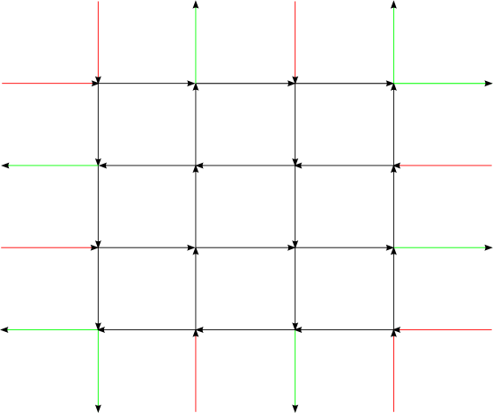
Figure 1: A grid network

In a road network, such bottlenecks as merging, diverging, and general junctions play a critical role in initiating, propagating, and dissipating traffic congestion. Some interesting traffic dynamics can be caused by interactions among these network bottlenecks: for examples, a beltway network can be totally gridlocked [12], and periodic oscillations can occur in a diverge-merge network [26]. Thus efforts are warranted to develop both physically realistic and mathematically tractable kinematic wave models of network traffic dynamics. Since traffic dynamics inside a link can be described by the LWR model and are well understood, the most important component of network kinematic wave models is related to how merging and diverging behaviors would impact the formation of shock and rarefaction waves at a general network junction shown in Figure 2, which has $m$ upstream links and $n$ downstream links. In the literature, there have been three lines of research into traffic dynamics through a general network junction. In the line of discrete Cell Transmission Model (CTM) [11; 34], boundary fluxes through a junction during a time interval are prescribed from adjacent cells’ conditions based on macroscopic merging and diverging rules. In the line of continuous models [25], shock and rarefaction waves on all links are analytically solved with jump initial conditions by decoupling the Riemann problem at the junction into $m+n$ Riemann problems on individual links. In the third line of continuous models [29], the discrete flux functions in CTM are used as decoupling conditions, and it was shown that the Riemann problem can be uniquely solved. The first two approaches bear their respective limitations: the CTM approach has been verified by empirical observations but cannot be applied to obtain such analytical insights as shock and rarefaction waves at a junction; the continuous model by [25] is mathematically tractable, but the decoupling method based on an optimization problem is not directly associated with any physical merging or diverging rules. In contrast, the third approach integrates the physical merging and diverging rules in CTM into the analytical framework of [25] is very promising for further studying network traffic dynamics.

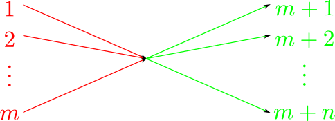
Figure 2: A general network junction

Since the kinematic wave model of network traffic flow is a system of hyperbolic conservation laws on a network structure, solutions to the Riemann problem at a junction, in which all links carry constant initial conditions, but discontinuities can occur at the junction, are of physical, analytical, and numerical importance: physically, they can define physical merging, diverging, and other behavioral rules; analytically, a system of hyperbolic conservation laws is well-defined if and only if the Riemann problem is uniquely solved [6]; and numerically, they can be incorporated into the Godunov finite difference equations [19]. In this study, we present a Riemann solver of the network kinematic wave model using the solution framework of [29]. Note that the Riemann solver is analytical in the sense of [15], different from numerical ones as discussed in [44]. The new solver is based on that in [25]: in the Riemann solutions, a stationary state arises on a link along with a shock or rarefaction wave, which is determined by the Riemann problem of the LWR model on the link with the initial and stationary states; the stationary state should be inside a feasible domain, such that the shock or rarefaction wave propagates backward on an upstream link and forward on a downstream link; and the constant in- or out-flux of a link equals the stationary flow-rate. The remaining piece in the Riemann solver is to introduce an entropy condition in the sense of [25] such that “this condition gives a unique solution at least for Riemann initial data”. But different from that in [25], the Riemann solver in this study uses a discrete flux function, which is defined in terms of upstream demands and downstream supplies, as an entropy condition. Such a discrete flux function is originally developed within the framework of CTM, models conflicts among merging and diverging traffic streams at the aggregate level, and is therefore a natural choice as the entropy condition to pick out unique physical solutions. To incorporate the new entropy condition, we enlarge the function space for weak solutions to the Riemann problem by introducing on each link an interior state, which is local and takes no space (of measure zero) right next to the junction. That is, the Riemann solution may be neither left- or right-continuous at jump discontinuities, and such a function space is still the same as that for traditional weak solutions. Then the entropy condition is introduced so that boundary fluxes through the junction be determined locally from interior states with numerical CTM flux functions. In addition, based on the equivalence between traffic density and the demand-supply pair, we solve the Riemann problem in the demand-supply space and show that stationary states exist and are unique. In this study, the local flux function is the global flux function derived in [29].

The rest of the paper is organized as follows. In Section 2, we present the network kinematic wave model and review Holden and Risebro’s Riemann solver and discrete CTM flux functions. In Section 3, we present a new Riemann solver. In Section 4, we solve the Riemann problem. In Section 5, we discuss some further properties of the Riemann solver. In Section 6, we present some concluding remarks.

2 A system of hyperbolic conservation laws at a network junction and the Riemann problem

In this study, we consider traffic dynamics in the junction network shown in Figure 2. We denote the set of upstream links by $A=\{1,\cdots,m\}$ and the set of downstream links by $B=\{m+1,\cdots,m+n\}$. For link $a\in A$, we introduce link coordinates $(a,x_{a})$, where $x_{a}\in(-\infty,0)$; for link $b\in B$, we introduce link coordinates $(b,x_{b})$, where $x_{b}\in(0,\infty)$. At a point $(a,x_{a})$ ($a\in A\cup B$) and time $t$, we denote the total density, speed, and flow-rate by $k_{a}(x_{a},t)$, $v_{a}(x_{a},t)$, and $q_{a}(x_{a},t)$, respectively. Hereafter we omit $(x_{a},t)$ from these variables unless necessary. Here we assume that vehicles of different paths, classes, or other attributes have the same characteristics, and that each link is homogeneous with a location-independent number of lanes, free-flow speeds, curvatures, slopes, and so on. Then we have the following fundamental diagram of flow-density and speed-density relations [20]:

$$v_{a} = V_{a}(k_{a}),$$

$$q_{a} = Q_{a}(k_{a})\equiv k_{a}V_{a}(k_{a}).$$

Generally, $Q_{a}(k_{a})$ is a unimodal function in $k_{a}$ and reaches its capacity, $C_{a}$, when traffic density equals the critical density $k_{a,c}$. If traffic density $k_{a}$ is strictly smaller than, equal to, or strictly greater than the critical density $k_{a,c}$, then we call the traffic state as strictly under-critical (SUC), critical (C), or strictly over-critical (SOC), respectively. An under-critical state (UC) can be SUC or C, and an over-critical state (OC) can be SOC or C. Note that different links can have different fundamental diagrams.

From traffic conservation, we have the following system of LWR models in the network [37; 43]

$${\frac{\partial{k_{a}}}{\partial{t}}}+{\frac{\partial{Q_{a}(k_{a})}}{\partial{x_{a}}}} = 0,\quad a\in A\cup B.$$ (1)

On a road link, it is well known that (1) admits weak solutions, among which the unique, physical solutions should satisfy so-called entropy conditions. For the LWR model, the traditional Lax’s entropy condition [33] is consistent with vehicles’ acceleration and deceleration behaviors [1].

On the network shown in Figure 2, (1) is a system of $m+n$ hyperbolic conservation laws, which can be understood as a semigroup based on the Godunov method and a Riemann solver [6]. Thus the main challenge of network kinematic wave theories is to develop a Riemann solver for the network, where hyperbolic conservation equations are coupled with each other at the junction due to merging and diverging conflicts among traffic streams. In the Riemann problem, we are interested in finding $k_{a}(x_{a},t)$ at any $(x_{a},t)$ from (1) with the following initial conditions with jump discontinuities at the junction:

$$k_{a}(x_{a},0) = k_{a},\quad x_{a}<0,\qquad a\in A$$ (2a)

$$k_{b}(x_{b},0) = k_{b},\quad x_{b}>0,\qquad b\in B$$ (2b)

For upstream link $a\in A$, we introduce a test function $\phi_{a}(x_{a},t):(-\infty,0]\times[0,\infty)$, which is smooth with compact support on $(-\infty,0]\times[0,\infty)$; for downstream link $b\in B$, we introduce a test function $\phi_{b}(x_{b},t):(0,\infty]\times[0,\infty)$, which is smooth with compact support on $(0,\infty]\times[0,\infty)$. These test functions are also smooth across the junction; i.e., $\phi_{a}(0,t)=\phi_{b}(0,t)$, and ${\frac{\partial{\phi_{a}}}{\partial{x_{a}}}}(0,t)={\frac{\partial{\phi_{b}}}{\partial{x_{b}}}}(0,t)$ for $a\in A$ and $b\in B$. Then we attempt to find the weak solutions to the Riemann problem of (1) with (2) in the following sense [9]:

$$\sum_{a\in A}\int_{0}^{\infty}\int_{-\infty}^{0}(k_{a}{\frac{\partial{\phi_{a}}}{\partial{t}}}+Q_{a}(k_{a}){\frac{\partial{\phi_{a}}}{\partial{x_{a}}}})dx_{a}dt+$$

$$\sum_{b\in B}\int_{0}^{\infty}\int_{0}^{\infty}(k_{b}{\frac{\partial{\phi_{b}}}{\partial{t}}}+Q_{b}(k_{b}){\frac{\partial{\phi_{b}}}{\partial{x_{b}}}})dx_{b}dt = 0.$$ (3)

2.1 Holden and Risebro’s Riemann solver

In [25], the Riemann problem of (1) with (2) was decoupled into $m+n$ Riemann problems of the LWR model based on the following observations. (1) Due to similarity in Riemann solutions; i.e., $k_{a}(x_{a},t)={\rho}_{a}(\frac{x_{a}}{t})$, a stationary state, $k_{a}^{*}$, initiates at the junction and spreads on link $a$ ($a\in A\cup B$). That is, for any $x_{a}\in(-\infty,0]$ ($a\in A$) or $x_{a}\in[0,\infty)$ ($a\in B$), $\lim_{t\to\infty}k_{a}(x_{a},t)=k_{a}^{*}$, and the stationary state pervades the whole link after a long time. Note that it is possible that the stationary state is the same as the initial state. It is stationary in the sense that the boundary flux of link $a$ is constant and equals

$$f_{a}=Q_{a}(k_{a}^{*}).$$

In addition, due to traffic conservation at the junction, we have

$$\sum_{a\in A}f_{a}=\sum_{b\in B}f_{b},$$

which is also the Rankine-Hugoniot condition for the junction. (2) A shock or rarefaction wave can develop on each link and solves the Riemann problem for the corresponding LWR model with initial and stationary states as initial data pairs. That is, for upstream link $a$ ($a\in A$), the shock or rarefaction wave solves ${\frac{\partial{k_{a}}}{\partial{t}}}+{\frac{\partial{Q_{a}(k_{a})}}{\partial{x_{a}}}}=0$ with $k_{a}(x_{a},0)={{\left\{\begin{array}[]{ll}k_{a},&x_{a}<0\\ k_{a}^{*},&x_{a}>0\end{array}\right.}}$; for downstream link $b$ ($b\in B$), the shock or rarefaction wave solves ${\frac{\partial{k_{b}}}{\partial{t}}}+{\frac{\partial{Q_{b}(k_{b})}}{\partial{x_{b}}}}=0$ with $k_{b}(x_{b},0)={{\left\{\begin{array}[]{ll}k_{b}^{*},&x_{b}<0\\ k_{b},&x_{b}>0\end{array}\right.}}$. Thus the Riemann problem is uniquely solved if and only if the stationary states are, and Holden and Risebro’s Riemann solver is equivalent to finding the following mapping [15]

$$(k_{1}^{*},\cdots,k_{m+n}^{*})={\mathbb{RS}}(k_{1},\cdots,k_{m+n}).$$ (4)

Since stationary states can only propagate backward on upstream links and forward on downstream links, feasible regions of stationary states can be obtained by analyzing the $m+n$ Riemann problems of the LWR model. Furthermore, as shown in [25], there can exist multiple feasible solutions of stationary states. Thus an additional entropy condition has to be introduced to give a unique solution to the Riemann problem of (1) with (2). In [25], an entropy of a junction is defined by $E=\sum_{a=1}^{m+n}g(\frac{f_{a}}{C_{a}})$, and it was proved that there exists a well-defined Riemann solver when $g(\cdot)$ is a strictly concave function. However, the entropy condition is not explicitly related to physical merging and diverging rules, and vehicles’ pre-defined route choices are not considered.

In [9], vehicles’ pre-defined route choices are introduced by a matrix of turning proportions $\xi_{a\to b}$ ($\forall a\in A,b\in B$), where $\xi_{a\to b}\in[0,1]$, and

$$\sum_{b\in B}\xi_{a\to b}=1,\quad a\in A.$$ (5)

Therefore, traffic conservation at the junction leads to $n$ equations: $\sum_{a\in A}f_{a}\xi_{a\to b}=f_{b}$ ($b\in B$). It was shown that the Riemann solver is well-defined for certain turning proportions. But this Riemann solver is not well-defined when $m>n$.

In [16; 17; 23; 21; 22], more Riemann solvers along this line have been proposed, but the entropy conditions are not directly related to merging and diverging behaviors in these studies.

2.2 Discrete CTM flux functions

In [11] and [34], the Godunov discrete form of the LWR model was extended to compute traffic flows through merging, diverging, and general junctions. In CTM, so-called traffic demand and supply, $d_{a}(x_{a},t)$ and $s_{a}(x_{a},t)$, are defined as functions of traffic density [14; 11; 34]

$$d_{a} = D_{a}(k_{a})\equiv Q_{a}(\min\{k_{a},k_{a,c}\}),$$ (6a)

$$s_{a} = S_{a}(k_{a})\equiv Q_{a}(\max\{k_{a},k_{a,c}\}),$$ (6b)

where traffic demand increases in total density $k_{a}$, and traffic supply decreases in total density $k_{a}$. Furthermore, $q_{a}=\min\{d_{a},s_{a}\}$, and $C_{a}=\max\{d_{a},s_{a}\}$. In addition, since $d_{a}/s_{a}$ is a strictly increasing function of $k_{a}$, $k_{a}$ can be uniquely determined by $d_{a}/s_{a}$. We denote this function by

$$k_{a} = K_{a}(d_{a}/s_{a}).$$ (7)

That is, the pair of demand and supply can uniquely determine the traffic state at a location and time.

Within the framework of CTM, boundary fluxes through a junction at time $t$ are be calculated as follows:

$$(f_{1}^{t},\cdots,f_{m+n}^{t})={\mathbb{FF}}^{0}(d_{1}^{t},\cdots,d_{m}^{t},s_{m+1}^{t},\cdots,s_{m+n}^{t}),$$ (8)

where $d_{1}^{t},\cdots,d_{m}^{t}$ are traffic demands in upstream cells next to the junction, $s_{m+1}^{t},\cdots,s_{m+n}^{t}$ are traffic supplies in downstream cells next to the junction, and $f_{1}^{t},\cdots,f_{m+n}^{t}$ are the out- and in-fluxes of all links. The discrete flux function (8) has been used to model traffic dynamics at various bottlenecks within the framework of CTM. For example, when vehicles have pre-defined route choices with turning proportions given in (5), a flux function was derived from the First-In-First-Out (FIFO) diverging and fair merging rules [32]. Other CTM merging and diverging models can be found in [28; 27].

Numerically, the flux functions (8) can be incorporated into discrete traffic conservation equations and simulate traffic dynamics in a road network with given initial and boundary conditions. Thus (8) can be considered as approximate, numerical Riemann solvers [36]. We can see that, using the concepts of demand and supply, it is rather straightforward to construct such flux functions for solving (1) numerically. While in many other systems of hyperbolic conservation laws, one has to solve the Riemann problem first and then obtain boundary fluxes as in the Godunov method. Physically, (8) models how the right of way at the junction is allocated among competing traffic streams and represents drivers’ macroscopic merging and diverging behaviors. Some of these macroscopic diverging and merging rules have been verified through observations [38; 35; 40; 8; 3].

3 A new Riemann solver

Since discrete flux functions (8) are both numerically and physically well-defined, it is reasonable to use it as an entropy condition to pick out unique, physical solution to the Riemann problem of (1) with (2). In [30; 28; 27; 29], a new analytical framework was proposed by replacing the entropy condition in [25] by various CTM flux functions in (8). In this section, we first describe the new framework and then focus on a new flux function derived in [29].

3.1 Riemann solvers with CTM flux functions as entropy conditions

In order to use CTM flux functions (8) as entropy conditions, we first enlarge the weak solution space by introducing a new interior state on each link in the Riemann solutions. That is, in the new weak solutions, we assume that $k_{a}(0,t)=k_{a}^{0}$, but $\lim_{t\to\infty}k_{a}(x_{a},t)=k_{a}^{*}$ for $x_{a}\in(-\infty,0)$ ($a\in A$) or $x_{a}\in(0,\infty)$ ($b\in B$). Such an interior state is right adjacent to the junction and takes a space of measure zero. Thus the new weak solutions to the Riemann problem still satisfy the traditional definition in (3). In addition, they do not impact shock or rarefaction waves on all links, which are determined by stationary and initial states.

Such interior states were first observed in numerical solutions of the Burgers equation [47; 7] and the LWR model [31] when stationary shock waves occur. Theoretically, if the LWR model ${\frac{\partial{k}}{\partial{t}}}+{\frac{\partial{Q(k)}}{\partial{x}}}=0$ on a line $x\in(-\infty,\infty)$ is solved by a zero-speed shock wave, then an interior state can be introduced at the stationary discontinuity without violating the definition of weak solutions or the Lax entropy condition. That is, $k(x,t)={{\left\{\begin{array}[]{ll}k_{L},&x<0\\ k_{M},&x=0\\ k_{R},&x>0\end{array}\right.}}$ with $k_{L}\leq k_{M}\leq k_{R}$ and $Q(k_{L})=Q(k_{R})$ is a feasible solution with a flimsy interior state $k_{M}$ at $x=0$. In reality, such an interior state can be observed at the interface of a stationary shock wave, if a detector covers a part of the upstream traffic stream and a part of the downstream traffic stream. Depending on the relative location of the detector, such an interior state may not be unique. Thus the interior states can physically exist, and the enlarged function space of weak solutions is still well defined. In addition, in [28; 27; 29], it was shown that the inclusion of interior states is necessary for Riemann solvers to be well-defined with some CTM flux functions. Thus the introduction of interior states into weak solutions makes both physical and mathematical senses. From the viewpoint of traffic flow modeling, the new framework is much more powerful and flexible, since it allows many flux functions derived from driving rules as entropy conditions.

Since discrete flux functions (8) are defined in demands and supplies, it is reasonable to use demand and supply, instead of density, as state variables in the new Riemann solver; i.e., traffic condition at $(x_{a},t)$ is determined by $U_{a}=(d_{a},s_{a})$. Thus a traffic state is UC if and only if $d_{a}\leq s_{a}=C_{a}$, or equivalently $U_{a}=(q_{a},C_{a})$; a traffic state is UC if and only if $s_{a}\leq d_{a}=C_{a}$, or equivalently $U_{a}=(C_{a},q_{a})$.

In the demand-supply space, we denote the initial and stationary traffic states on link $a$ by $(d_{a},s_{a})$ and $(d_{a}^{*},s_{a}^{*})$, respectively. Then we have the following observations in the Riemann solutions:

$$f_{a} = \min\{d_{a}^{*},s_{a}^{*}\},\quad a\in A\cup B$$ (9a)

In addition, we have the following lemma regarding the feasible regions of stationary states.

Lemma 3.1

[29] In demand-supply space, the feasible regions of stationary states are given by

$$U_{a}^{*} \in {\mathbb{B}}(U_{a},\cdot)\equiv(d_{a},C_{a})\cup\{(C_{a},s_{a}^{*})|s_{a}^{*}<d_{a}\},\quad a\in A$$ (9b)

$$U_{b}^{*} \in {\mathbb{F}}(\cdot,U_{b})\equiv(C_{b},s_{b})\cup\{(d_{b}^{*},C_{b})|d_{b}^{*}<s_{b}\},\quad b\in B$$ (9c)

which lead to

$$f_{a} \leq d_{a},\quad a\in A$$ (9e)

$$f_{b} \leq s_{b},\quad b\in B$$ (9f)

Further, we denote the interior state on link $a$ by $U_{a}^{0}$ ($a\in A\cup B$). Since interior states do not propagate into road links, the Riemann problems with stationary and interior states as initial data are solved by waves, whose speeds are positive on the upstream links and negative on the downstream links. Therefore, in supply-demand space, the feasible regions of interior states are given by

$$U_{a}^{0}\in{\mathbb{F}}(U_{a}^{*},\cdot)\equiv\{(C_{a},s_{a}^{*})|s_{a}^{*}<d_{a}^{*}=C_{a}\}\cup\{(d_{a}^{0},s_{a}^{0})|s_{a}^{0}\geq d_{a}^{*},d_{a}^{*}\leq s_{a}^{*}=C_{a}\},$$ (10a)

$$U_{b}^{0}\in{\mathbb{B}}(\cdot,U_{b}^{*})\equiv\{(d_{b}^{*},C_{b})|d_{b}^{*}<s_{b}^{*}=C_{b}\}\cup\{(d_{b}^{0},s_{b}^{0})|d_{b}^{0}\geq s_{b}^{*},s_{b}^{*}\leq d_{b}^{*}=C_{b}\}.$$ (10b)

where $a\in A$ and $b\in B$. When $U_{a}^{0}=U_{a}^{*}$, interior states do not exist.

From the feasible regions of stationary and interior states in (9) and (10), we have the following corollary.

Corollary 3.2

For upstream link $a\in A$, $U_{a}^{*}$ is SOC if and only if $f_{a}<d_{a}$, and $U_{a}^{*}$ is UC if and only if $f_{a}=d_{a}$. In addition, if $U_{a}^{*}$ is SOC, then $U_{a}^{*}=U_{a}^{0}=(C_{a},f_{a})$; if $U_{a}^{*}$ is UC, then $U_{a}^{*}=(d_{a},C_{a})$, and $U_{a}^{0}=(d_{a}^{0},s_{a}^{0})$ with $s_{a}^{0}\geq d_{a}$. For downstream link $b\in B$, $U_{b}^{*}$ is SUC if and only if $f_{b}<s_{b}$, and $U_{b}^{*}$ is OC if and only if $f_{b}=s_{b}$. In addition, if $U_{b}^{*}$ is SUC, then $U_{b}^{*}=U_{b}^{0}=(f_{b},C_{b})$; if $U_{b}^{*}$ is OC, then $U_{b}^{*}=(C_{b},s_{b})$, and $U_{b}^{0}=(d_{b}^{0},s_{b}^{0})$ with $d_{b}^{0}\geq s_{b}$.

Here we define four ratios for upstream link $a\in A$: the initial demand level $\delta_{a}=\frac{d_{a}}{C_{a}}$, the stationary demand level $\delta^{*}_{a}=\frac{d_{a}^{*}}{C_{a}}$, the interior demand level $\delta^{0}_{a}=\frac{d_{a}^{0}}{C_{a}}$, and the flux level $\tilde{\delta}_{a}=\frac{f_{a}}{C_{a}}$. Then we have the following results.

Corollary 3.3

$U_{a}^{*}$ for $a\in A$ is SOC if and only if $\tilde{\delta}_{a}<\delta_{a}$; and $U_{a}^{*}$ is UC if and only if $\tilde{\delta}_{a}=\delta_{a}$. In addition, if $U_{a}^{*}$ is SOC, then

$$1=\delta^{0}_{a}=\delta^{*}_{a}\geq\delta_{a}>\tilde{\delta}_{a};$$

if $U_{a}^{*}$ is UC, then

$$\delta^{*}_{a}=\delta_{a}=\tilde{\delta}_{a}.$$

Note that the relationship between $\delta^{0}_{a}$ and other demand levels when $U_{a}^{*}$ is UC is to be determined.

Similarly we define four ratios for downstream link $b\in B$: the initial supply level $\sigma_{b}=\frac{s_{b}}{C_{b}}$, the stationary supply level $\sigma^{*}_{b}=\frac{s_{b}^{*}}{C_{b}}$, the interior supply level $\sigma^{0}_{b}=\frac{s_{b}^{0}}{C_{b}}$, and the flux level $\tilde{\sigma}_{b}=\frac{f_{b}}{C_{b}}$. Then we have the following results.

Corollary 3.4

$U_{b}^{*}$ for $b\in B$ is SUC if and only if $\tilde{\sigma}_{b}<\sigma_{b}$; and $U_{b}^{*}$ is OC if and only if $\tilde{\sigma}_{b}=\sigma_{b}$. In addition, if $U_{b}^{*}$ is SUC, then

$$1=\sigma^{0}_{b}=\sigma^{*}_{b}\geq\sigma_{b}>\tilde{\sigma}_{b};$$

if $U_{b}^{*}$ is OC, then

$$\sigma^{*}_{b}=\sigma_{b}=\tilde{\sigma}_{b}.$$

Note that the relationship between $\sigma^{0}_{b}$ and other supply levels when $U_{b}^{*}$ is OC is to be determined.

In the new Riemann solvers, various CTM flux functions in (8) are used to determine fluxes locally from interior states as follows:

$$(f_{1},\cdots,f_{m+n})={\mathbb{FF}}^{0}(d_{1}^{0},\cdots,d_{m}^{0},s_{m+1}^{0},\cdots,s_{m+n}^{0}).$$ (11)

From the corollaries above, we can see that, given initial upstream demands, $d_{a}$ ($a\in A$), and downstream supplies, $s_{b}$ ($b\in B$), if one can find all boundary fluxes, $f_{a}$ and $f_{b}$, then the stationary states can be uniquely determined. But the interior states may not be uniquely determined. Thus the Riemann problem is uniquely solved in the sense that all stationary states and waves on all links are uniquely solved. Therefore, the Riemann problem is uniquely solved if and only if, from (9), (10), and (11), we can find a unique flux function that maps initial conditions into boundary fluxes

$$(f_{1},\cdots,f_{m+n}) = {\mathbb{FF}}(d_{1},\cdots,d_{m},s_{m+1},\cdots,s_{m+n}).$$ (12)

Hereafter, we refer to ${\mathbb{FF}}^{0}(\cdots)$ in (11) as local or discrete flux functions and ${\mathbb{FF}}(\cdots)$ in (12) as global or continuous flux functions. Obviously, ${\mathbb{FF}}(\cdots)$ is the Godunov flux function, since it is derived from Riemann solutions.

Then from Corollary 3.2, we obtain the corresponding demand-supply Riemann solver, which maps upstream demands and downstream supplies into stationary states:

$$(U_{1}^{*},\cdots,U_{m+n}^{*}) = {\mathbb{RS}}^{\prime}(d_{1},\cdots,d_{m},s_{m+1},\cdots,s_{m+n}).$$ (13)

Since both demand and supply are many-to-one functions of density, it suggests that different initial densities could lead to the same stationary states, if and only if the corresponding upstream demands and downstream supplies are the same. From ${\mathbb{RS}}^{\prime}(\cdots)$ we can obtain the traditional Riemann solver ${\mathbb{RS}}(\cdots)$ in (4) by first converting $(k_{1},\cdots,k_{m+n})$ into $(d_{1},\cdots,d_{m},s_{m+1},\cdots,s_{m+n})$, then applying (13) to find stationary demands and supplies, and finally converting $(U_{1}^{*},\cdots,U_{m+n}^{*})$ into $(k_{1}^{*},\cdots,k_{m+n}^{*})$ using (7). However, from the traditional Riemann solver one may not be able to obtain a demand-supply Riemann solver. It can be seen that a Riemann solver in (13) satisfies the consistency condition [15], if and only if ${\mathbb{FF}}(d_{1},\cdots,d_{m},s_{m+1},\cdots,s_{m+n})={\mathbb{FF}}(d_{1}^{*},\cdots,d_{m}^{*},s_{m+1}^{*},\cdots,s_{m+n}^{*})$, which is equivalent to that $(U_{1}^{*},\cdots,U_{m+n}^{*})={\mathbb{RS}}^{\prime}(d_{1}^{*},\cdots,d_{m}^{*},s_{m+1}^{*},\cdots,s_{m+n}^{*})$. In addition, we call the local or discrete flux function ${\mathbb{FF}}^{0}(\cdots)$ invariant if ${\mathbb{FF}}^{0}(\cdots)={\mathbb{FF}}(\cdots)$.

3.2 A new local flux function

In this study, we use the Godunov flux function in [29] as a new local flux function, (11). Note that the discrete flux function in [29] is consistent with fair merging and first-in-first-out diverging rules but different from the Godunov flux function. Here all vehicles have predefined route choices, and the turning proportions, $\xi_{a\to b}$, are given in (5). The discrete flux function ${\mathbb{FF}}^{0}(\cdots)$ is defined as follows:

1. The out-flux of upstream link $a\in A$ is given by

   $$f_{a} = \min\{d_{a}^{0},\theta^{0}C_{a}\},$$ (14a)

   where the interior critical demand level, $$\theta^{0}$$, is defined as follows:

   $$\theta^{0} = \min\left\{\max_{a\in A}\frac{d_{a}^{0}}{C_{a}},\min_{b\in B}\max_{A_{1}\subseteq A}\frac{s^{0}_{b}-\sum_{{\alpha}\in A\setminus A_{1}}d_{\alpha}^{0}\xi_{{\alpha}\to b}}{\sum_{a\in A_{1}}C_{a}\xi_{a\to b}}\right\},$$ (14b)

   where $$A_{1}$$ is not empty.

2. The in-flux of downstream link $b\in B$ is given by

   $$f_{b} = \sum_{a\in A}f_{a}\xi_{a\to b}.$$ (14c)

In terms of demand and supply levels, ${\mathbb{FF}}^{0}(\cdots)$ in (14) can be re-written as

$$\tilde{\delta}_{a} = \min\{\delta_{a}^{0},\theta^{0}\},$$ (15a)

$$\theta^{0} = \min\left\{\max_{a\in A}\delta_{a}^{0},\min_{b\in B}\max_{A_{1}\subseteq A}\frac{C_{b}\sigma^{0}_{b}-\sum_{{\alpha}\in A\setminus A_{1}}C_{{\alpha}\to b}\delta_{\alpha}^{0}}{\sum_{a\in A_{1}}C_{a\to b}}\right\},$$ (15b)

$$C_{b}\tilde{\sigma}_{b} = \sum_{a\in A}C_{a\to b}\tilde{\delta}_{a},$$ (15c)

where $C_{a\to b}=C_{a}\xi_{a\to b}$ for $a\in A$ and $b\in B$.

3.3 Average demand levels

In this subsection, we discuss properties of $\theta^{0}$ in (15b). For $a\in A$ and $b\in B$, we define the demand and supply levels by $\mu_{a}\in[0,1]$ and $\nu_{b}\in[0,1]$, respectively. Further, we denote $\pi_{b}=C_{b}\nu_{b}-\sum_{a\in A}C_{a\to b}\mu_{a}$. We denote the vector of $\mu_{a}$ for $a\in A$ by $\mu$$\mu$$\mu$, and the vector of $\nu_{b}$ for $b\in B$ by $\nu$$\nu$$\nu$. We define the average demand level of set $A_{1}$ for link $b$ by

$$\gamma_{b}(A_{1}) = \frac{C_{b}\nu_{b}-\sum_{{\alpha}\in A\setminus A_{1}}C_{{\alpha}\to b}\mu_{\alpha}}{\sum_{a\in A_{1}}C_{a\to b}}=\frac{\pi_{b}+\sum_{a\in A_{1}}C_{a\to b}\mu_{a}}{\sum_{a\in A_{1}}C_{a\to b}},$$ (16)

where $A_{1}\subseteq A$ is non-empty.

Lemma 3.5

For ${\alpha}\in A_{1}$, and $A_{2}\equiv A_{1}\setminus\{{\alpha}\}\neq\emptyset$, if $\mu_{\alpha}>,=,<\gamma_{b}(A_{1})$, then $\gamma_{b}(A_{2})<,=,>\gamma_{b}(A_{1})$, and $\mu_{\alpha}>,=,<\gamma_{b}(A_{2})$, respectively. For ${\alpha}\notin A_{1}$, and $A_{2}\equiv A_{1}\cup\{{\alpha}\}$, if $\mu_{\alpha}<,=,>\gamma_{b}(A_{1})$, then $\gamma_{b}(A_{2})<,=,>\gamma_{b}(A_{1})$, and $\mu_{\alpha}<,=,>\gamma_{b}(A_{2})$, respectively. That is, if we remove a link with a larger demand level, then the average demand level decreases; if we add a link with a larger demand level, then the average demand level increases.

Proof. For ${\alpha}\in A_{1}$, and $A_{2}\equiv A_{1}\setminus\{{\alpha}\}\neq\emptyset$, we have

$$\gamma_{b}(A_{1}) = \frac{\sum_{a\in A_{2}}C_{a\to b}\mu_{a}+C_{{\alpha}\to b}\mu_{\alpha}+\pi_{b}}{\sum_{a\in A_{2}}C_{a\to b}+C_{{\alpha}\to b}},$$

which leads to

$$\gamma_{b}(A_{2}) = \frac{\sum_{a\in A_{2}}C_{a\to b}\mu_{a}+\pi_{b}}{\sum_{a\in A_{2}}C_{a\to b}}=\gamma_{b}(A_{1})+\frac{(\gamma_{b}(A_{1})-\mu_{\alpha})C_{{\alpha}\to b}}{\sum_{a\in A_{2}}C_{a\to b}},$$

Thus, if $\mu_{\alpha}>,=,<\gamma_{b}(A_{1})$, then $\gamma_{b}(A_{2})<,=,>\gamma_{b}(A_{1})$, and $\mu_{\alpha}>,=,<\gamma_{b}(A_{2})$, respectively.

For ${\alpha}\notin A_{1}$, and $A_{2}\equiv A_{1}\cup\{{\alpha}\}$, we have

$$\gamma_{b}(A_{1}) = \frac{\sum_{a\in A_{2}}C_{a\to b}\mu_{a}-C_{{\alpha}\to b}\mu_{\alpha}+\pi_{b}}{\sum_{a\in A_{2}}C_{a\to b}-C_{{\alpha}\to b}},$$

which leads to

$$\gamma_{b}(A_{2}) = \frac{\sum_{a\in A_{2}}C_{a\to b}\mu_{a}+\pi_{b}}{\sum_{a\in A_{2}}C_{a\to b}}=\gamma_{b}(A_{1})-\frac{(\gamma_{b}(A_{1})-\mu_{\alpha})C_{{\alpha}\to b}}{\sum_{a\in A_{2}}C_{a\to b}}.$$

Thus, if $\mu_{\alpha}<,=,>\gamma_{b}(A_{1})$, $\gamma_{b}(A_{2})<,=,>\gamma_{b}(A_{1})$, respectively. Furthermore,

$$(\gamma_{b}(A_{2})-\mu_{\alpha})\sum_{a\in A_{2}}C_{a\to b} = \sum_{a\in A_{1}}C_{a\to b}\mu_{a}+C_{{\alpha}\to b}\mu_{\alpha}+\pi_{b}-\mu_{\alpha}\sum_{a\in A_{1}}C_{a\to b}-C_{{\alpha}\to b}\mu_{\alpha}$$

$$= \sum_{a\in A_{1}}C_{a\to b}\mu_{a}+\pi_{b}-\mu_{\alpha}\sum_{a\in A_{1}}C_{a\to b}=(\gamma_{b}(A_{1})-\mu_{\alpha})\sum_{a\in A_{1}}C_{a\to b}.$$

Thus, if $\mu_{\alpha}<,=,>\gamma_{b}(A_{1})$, $\mu_{\alpha}<,=,>\gamma_{b}(A_{2})$, respectively. $\blacksquare$

We denote the maximum average demand level for link $b$ by $\Gamma_{b}=\max_{A_{1}\subseteq A,A_{1}\neq\emptyset}\gamma_{b}(A_{1})$, which has the following properties.

Lemma 3.6

$\gamma_{b}(A_{1})$ and $\Gamma_{b}$ have the following properties.

1. When $\pi_{b}>0$, then $\gamma_{b}(\{a\})>\mu_{a}$ for $a\in A$, and $\Gamma_{b}=\max_{a\in A}\gamma_{b}(\{a\})>\max_{a\in A}\mu_{a}$.

2. When $\pi_{b}=0$, then $\gamma_{b}(\{a\})=\mu_{a}$ for $a\in A$, and $\Gamma_{b}=\max_{a\in A}\gamma_{b}(\{a\})=\max_{a\in A}\mu_{a}$.

3. When $\pi_{b}<0$, then $\gamma_{b}(\{a\})<\mu_{a}$ for $a\in A$, and there exists a unique $A_{1}\neq\emptyset$, such that $\Gamma_{b}=\gamma_{b}(A_{1})$, $\mu_{a}>\Gamma_{b}\geq\mu_{\alpha}$ for $a\in A_{1}$ and ${\alpha}\in A\setminus A_{1}$.

Proof.

1. When $\pi_{b}>0$, from (16), we can have $\gamma_{b}(\{a\})>\mu_{a}$ for $a\in A$. Then from Lemma 3.5 we have $\min_{a\in A_{1}}\mu_{a}<\gamma_{b}(A_{1})\leq\max_{a\in A_{1}}\gamma_{b}(\{a\})$. Thus $\Gamma_{b}=\max_{a\in A}\gamma_{b}(\{a\})>\max_{a\in A}\mu_{a}$. Note that $\max_{a\in A}\gamma_{b}(\{a\})$ and $\max_{a\in A}\mu_{a}$ may attain their maxima for different $a$.

2. When $\pi_{b}=0$, from (16), we can have $\gamma_{b}(\{a\})=\mu_{a}$ for $a\in A$. Then from Lemma 3.5 we have $\min_{a\in A_{1}}\mu_{a}\leq\gamma_{b}(A_{1})\leq\max_{a\in A_{1}}\mu_{a}$. Thus $\Gamma_{b}=\max_{a\in A}\gamma_{b}(\{a\})=\max_{a\in A}\mu_{a}$.

3. When $\pi_{b}<0$, from (16), we can have $\gamma_{b}(\{a\})<\mu_{a}$ for $a\in A$. Since $A$ has a finite number of subsets $A_{1}$, $\Gamma_{b}$ exists and we can find $A_{1}$, such that $\Gamma_{b}=\gamma_{b}(A_{1})$, and the value of $\Gamma_{b}$ is unique. First, for ${\alpha}\notin A_{1}$, $\mu_{\alpha}\leq\gamma_{b}(A_{1})$, since, otherwise, from Lemma 3.5 we have $\gamma_{b}(A_{1})<\gamma_{b}(A_{1}\cup\{{\alpha}\})$, which contradicts that $\Gamma_{b}=\gamma_{b}(A_{1})$. Second, there exists at least one $a\in A_{1}$, such that $\mu_{a}>\gamma_{b}(A_{1})$, since, otherwise, from Lemma 3.5 we have $\gamma_{b}(\{a\})=\mu_{a}$ for all $a\in A_{1}$, which contradicts that $\gamma_{b}(\{a\})<\mu_{a}$. Third, for all $a\in A_{1}$, $\mu_{a}\geq\gamma_{b}(A_{1})$, since, otherwise, from Lemma 3.5 we have $\gamma_{b}(A_{1})<\gamma_{b}(A_{1}\setminus\{a\})$, which contradicts that $\Gamma_{b}=\gamma_{b}(A_{1})$. Assume that $a\in A_{1}^{*}\subset A_{1}$ and $\mu_{a}>\gamma_{b}(A_{1})$, then $\mu_{\alpha}=\gamma_{b}(A_{1})$ for ${\alpha}\in A_{1}\setminus A_{1}^{*}$, and $\gamma_{b}(A_{1}^{*})=\gamma_{b}(A_{1})$. Since $A_{1}^{*}\neq\emptyset$ is unique, there exists a unique $A_{1}=A_{1}^{*}\neq\emptyset$, such that $\Gamma_{b}=\gamma_{b}(A_{1})$, $\mu_{a}>\Gamma_{b}\geq\mu_{\alpha}$ for $a\in A_{1}$ and ${\alpha}\in A\setminus A_{1}$.

$\blacksquare$

Assuming that $\mu_{a}$ ($a\in A$) are in a decreasing order; i.e., $\mu_{1}\geq\cdots\geq\mu_{m}$, we define the following average demand level of the first $l$ upstream links:

$$\gamma_{b}(l) = \gamma_{b}(\{1,\cdots,l\}).$$

Then we have the following corollary.

Corollary 3.7

$\gamma_{b}(l)$ and $\Gamma_{b}$ have the following properties:

1. When $\pi_{b}>0$, $\gamma_{b}(l)>\mu_{l}$ for $l\in A$, $\gamma_{b}(1)>\cdots>\gamma_{b}(m)$, and $\Gamma_{b}=\max_{a\in A}\gamma_{b}(\{a\})\geq\gamma_{b}(1)>\mu_{1}$.

2. When $\pi_{b}=0$, $\gamma_{b}(l)\geq\mu_{l}$ for $l\in A$, $\gamma_{b}(1)\geq\cdots\geq\gamma_{b}(m)$, and $\Gamma_{b}=\mu_{1}$.

3. When $\pi_{b}<0$, there exists a unique $l^{*}\in\{1,\cdots,m\}$, such that $\gamma_{b}(1)<\cdots<\gamma_{b}(l^{*})\geq\gamma_{b}(l^{*}+1)\geq\cdots\geq\gamma_{b}(m)$, $\gamma_{b}(l)<\mu_{l}$ for $l=1,\cdots,l^{*}$, and $\gamma_{b}(l)\geq\mu_{l}$ for $l=l^{*}+1,\cdots,m$. That is, for every $b$, there exists a unique $l^{*}_{b}$ solving $\min l$, such that $\gamma_{b}(l)\geq\gamma_{b}(l+1)$. In addition, $l^{*}_{b}=1$ and $\gamma_{b}(1)\geq\mu_{1}$ if and only if $\pi_{b}\geq 0$.

Proof. When $\pi_{b}\geq 0$, the results are obvious. Here we will focus on $\pi_{b}<0$. We denote $l^{*}$ as the number of links in $A_{1}$, where $\Gamma_{b}=\gamma_{b}(A_{1})$ and $\mu_{a}>\Gamma_{b}\geq\mu_{\alpha}$ for $a\in A_{1}$ and ${\alpha}\in A\setminus A_{1}$. Then $l^{*}$ is unique, and $\mu_{l^{*}}>\Gamma_{b}=\gamma_{b}(l^{*})\geq\mu_{b}(l^{*}+1)$. From Lemma 3.5, we have $\gamma_{b}(1)<\cdots<\gamma_{b}(l^{*})\geq\gamma_{b}(l^{*}+1)\geq\cdots\geq\gamma_{b}(m)$, $\gamma_{b}(l)<\mu_{l}$ for $l=1,\cdots,l^{*}$, and $\gamma_{b}(l)\geq\mu_{l}$ for $l=l^{*}+1,\cdots,m$. $\blacksquare$

We define the critical demand level by

$$g(\kern-0.24994pt\hbox{$\mu$}\kern-6.02548pt\kern 0.50003pt\hbox{$\mu$}\kern-6.02548pt\kern-0.24994pt\raise 0.43304pt\hbox{$\mu$},\kern-0.24994pt\hbox{$\nu$}\kern-4.93982pt\kern 0.50003pt\hbox{$\nu$}\kern-4.93982pt\kern-0.24994pt\raise 0.43304pt\hbox{$\nu$}) = \min_{b}\max_{A_{1}}\frac{C_{b}\nu_{b}-\sum_{{\alpha}\in A\setminus A_{1}}C_{{\alpha}\to b}\mu_{\alpha}}{\sum_{a\in A_{1}}C_{a\to b}}$$ (17)

$$= \min_{b}\max_{A_{1}}\frac{\pi_{b}+\sum_{a\in A_{1}}C_{a\to b}\mu_{a}}{\sum_{a\in A_{1}}C_{a\to b}}$$

Since $g(\kern-0.24994pt\hbox{$\mu$}\kern-6.02548pt\kern 0.50003pt\hbox{$\mu$}\kern-6.02548pt\kern-0.24994pt\raise 0.43304pt\hbox{$\mu$},\kern-0.24994pt\hbox{$\nu$}\kern-4.93982pt\kern 0.50003pt\hbox{$\nu$}\kern-4.93982pt\kern-0.24994pt\raise 0.43304pt\hbox{$\nu$})=\min_{b}\Gamma_{b}$, we have the following theorem regarding $g(\kern-0.24994pt\hbox{$\mu$}\kern-6.02548pt\kern 0.50003pt\hbox{$\mu$}\kern-6.02548pt\kern-0.24994pt\raise 0.43304pt\hbox{$\mu$},\kern-0.24994pt\hbox{$\nu$}\kern-4.93982pt\kern 0.50003pt\hbox{$\nu$}\kern-4.93982pt\kern-0.24994pt\raise 0.43304pt\hbox{$\nu$})$.

Theorem 3.8

For $C_{a\to b}>0$, $C_{b}>0$, $\mu_{a}\in[0,1]$, and $\nu_{b}\in[0,1]$ ($a\in A$ and $b\in B$), $g(\kern-0.24994pt\hbox{$\mu$}\kern-6.02548pt\kern 0.50003pt\hbox{$\mu$}\kern-6.02548pt\kern-0.24994pt\raise 0.43304pt\hbox{$\mu$},\kern-0.24994pt\hbox{$\nu$}\kern-4.93982pt\kern 0.50003pt\hbox{$\nu$}\kern-4.93982pt\kern-0.24994pt\raise 0.43304pt\hbox{$\nu$})$ defined in (17) has the following properties:

1. $g(\kern-0.24994pt\hbox{$\mu$}\kern-6.02548pt\kern 0.50003pt\hbox{$\mu$}\kern-6.02548pt\kern-0.24994pt\raise 0.43304pt\hbox{$\mu$},\kern-0.24994pt\hbox{$\nu$}\kern-4.93982pt\kern 0.50003pt\hbox{$\nu$}\kern-4.93982pt\kern-0.24994pt\raise 0.43304pt\hbox{$\nu$})\geq\max_{a}\mu_{a}$ if and only if $\min_{b\in B}\pi_{b}\geq 0$.

2. If and only if $\min_{b\in B}\pi_{b}<0$, there exists a unique non-empty $A_{*}\subseteq A$ such that

   $$g(\kern-0.24994pt\hbox{$\mu$}\kern-6.02548pt\kern 0.50003pt\hbox{$\mu$}\kern-6.02548pt\kern-0.24994pt\raise 0.43304pt\hbox{$\mu$},\kern-0.24994pt\hbox{$\nu$}\kern-4.93982pt\kern 0.50003pt\hbox{$\nu$}\kern-4.93982pt\kern-0.24994pt\raise 0.43304pt\hbox{$\nu$}) = \min_{b}\max_{A_{1}}\gamma_{b}(A_{1})=\min_{b}\gamma_{b}(A_{*})=\max_{A_{1}}\min_{b}\gamma_{b}(A_{1}),$$ (18)

   and

   $$\min_{a\in A_{*}}\mu_{a}>g(\kern-0.24994pt\hbox{$\mu$}\kern-6.02548pt\kern 0.50003pt\hbox{$\mu$}\kern-6.02548pt\kern-0.24994pt\raise 0.43304pt\hbox{$\mu$},\kern-0.24994pt\hbox{$\nu$}\kern-4.93982pt\kern 0.50003pt\hbox{$\nu$}\kern-4.93982pt\kern-0.24994pt\raise 0.43304pt\hbox{$\nu$})\geq\max_{{\alpha}\in A\setminus A_{*}}\mu_{a}.$$

Proof. When $\min_{b}\pi_{b}\geq 0$, from Lemma 3.6 we have $g(\kern-0.24994pt\hbox{$\mu$}\kern-6.02548pt\kern 0.50003pt\hbox{$\mu$}\kern-6.02548pt\kern-0.24994pt\raise 0.43304pt\hbox{$\mu$},\kern-0.24994pt\hbox{$\nu$}\kern-4.93982pt\kern 0.50003pt\hbox{$\nu$}\kern-4.93982pt\kern-0.24994pt\raise 0.43304pt\hbox{$\nu$})=\min_{b}\Gamma_{b}\geq\max_{a}\mu_{a}$.

When $\min_{b}\pi_{b}<0$, we denote $A_{b}=\{a\in A|\mu_{a}>\Gamma_{b}\}$. From Lemma 3.6, $A_{b}=\emptyset$ if and only if $\pi_{b}\geq 0$. We denote $A_{*}=\cup_{b\in B}A_{b}\neq\emptyset$, since $\min_{b}\pi_{b}<0$. In addition, for any $a\in A_{*}$, $\mu_{a}>\min_{b}\Gamma_{b}=g(\kern-0.24994pt\hbox{$\mu$}\kern-6.02548pt\kern 0.50003pt\hbox{$\mu$}\kern-6.02548pt\kern-0.24994pt\raise 0.43304pt\hbox{$\mu$},\kern-0.24994pt\hbox{$\nu$}\kern-4.93982pt\kern 0.50003pt\hbox{$\nu$}\kern-4.93982pt\kern-0.24994pt\raise 0.43304pt\hbox{$\nu$})$; and for any ${\alpha}\in A\setminus A_{*}$, $\mu_{a}\leq\min_{b}\Gamma_{b}=g(\kern-0.24994pt\hbox{$\mu$}\kern-6.02548pt\kern 0.50003pt\hbox{$\mu$}\kern-6.02548pt\kern-0.24994pt\raise 0.43304pt\hbox{$\mu$},\kern-0.24994pt\hbox{$\nu$}\kern-4.93982pt\kern 0.50003pt\hbox{$\nu$}\kern-4.93982pt\kern-0.24994pt\raise 0.43304pt\hbox{$\nu$})$. In addition, $g(\kern-0.24994pt\hbox{$\mu$}\kern-6.02548pt\kern 0.50003pt\hbox{$\mu$}\kern-6.02548pt\kern-0.24994pt\raise 0.43304pt\hbox{$\mu$},\kern-0.24994pt\hbox{$\nu$}\kern-4.93982pt\kern 0.50003pt\hbox{$\nu$}\kern-4.93982pt\kern-0.24994pt\raise 0.43304pt\hbox{$\nu$})=\min_{b}\gamma_{b}(A_{*})$, and $\min_{a\in A_{*}}\mu_{a}>\min_{b}\gamma_{b}(A_{*})\geq\max_{{\alpha}\in A\setminus A_{*}}\mu_{a}$.

Since $\min_{b}\pi_{b}<0$, we have $\min_{b}\gamma_{b}(\{a\})<\mu_{a}$ for $a\in A$. Since $A$ has a finite number of subsets $A_{1}$, thus we can find $A_{1}^{*}$ such that $\max_{A_{1}}\min_{b}\gamma_{b}(A_{1})=\min_{b}\gamma_{b}(A_{1}^{*})$, and the maximum value is unique. First, for any ${\alpha}\notin A_{1}^{*}$ $\mu_{\alpha}\leq\min_{b}\gamma_{b}(A_{1}^{*})$, since, otherwise, from Lemma 3.5 $\min_{b}\gamma_{b}(A_{1}^{*}\cup\{{\alpha}\})>\min_{b}\gamma_{b}(A_{1}^{*})$. Thus $a\in A_{1}^{*}$ if $\mu_{a}>\min_{b}\gamma_{b}(A_{1}^{*})$. Second, there exists at least one $a\in A_{1}^{*}$, such that $\mu_{a}>\min_{b}\gamma_{b}(A_{1}^{*})$, since, otherwise, $\mu_{a}\leq\min_{b}\gamma_{b}(A_{1}^{*})$ for all $a\in A_{1}^{*}$, and from Lemma 3.5 $\mu_{a}\leq\min_{b}\gamma_{b}(\{a\})$, which is not possible. Third, if $a\in A_{1}^{*}$, then $\mu_{a}\geq\min_{b}\gamma_{b}(A_{1}^{*})$, since, otherwise, from Lemma 3.5 $\min_{b}\gamma_{b}(A_{1}^{*}\setminus\{a\})>\min_{b}\gamma_{b}(A_{1}^{*})$. Therefore, without loss of generality, we can remove all $a$ from $A_{1}^{*}$ if $\mu_{a}=\min_{b}\gamma_{b}(A_{1}^{*})$, and the value of $\min_{b}\gamma_{b}(A_{1}^{*})$ does not change. Then $A_{1}^{*}=\{a\in A|\mu_{a}>\min_{b}\gamma_{b}(A_{1}^{*})\}$ is unique; that is, there exists a unique $A_{1}^{*}$ such that $\min_{a\in A_{1}^{*}}\mu_{a}>\min_{b}\gamma_{b}(A_{1}^{*})\geq\max_{{\alpha}\in A\setminus A_{1}^{*}}\mu_{\alpha}$.

Therefore, $A_{*}=A_{1}^{*}$, and (18) is proved. $\blacksquare$

From Theorem 3.8 we have the following corollary.

Corollary 3.9

If $\mu_{a}$ is decreasingly ordered, we have the following results on $g(\kern-0.24994pt\hbox{$\mu$}\kern-6.02548pt\kern 0.50003pt\hbox{$\mu$}\kern-6.02548pt\kern-0.24994pt\raise 0.43304pt\hbox{$\mu$},\kern-0.24994pt\hbox{$\nu$}\kern-4.93982pt\kern 0.50003pt\hbox{$\nu$}\kern-4.93982pt\kern-0.24994pt\raise 0.43304pt\hbox{$\nu$})$:

1. If and only if $\min_{b}\pi_{b}\geq 0$, $g(\kern-0.24994pt\hbox{$\mu$}\kern-6.02548pt\kern 0.50003pt\hbox{$\mu$}\kern-6.02548pt\kern-0.24994pt\raise 0.43304pt\hbox{$\mu$},\kern-0.24994pt\hbox{$\nu$}\kern-4.93982pt\kern 0.50003pt\hbox{$\nu$}\kern-4.93982pt\kern-0.24994pt\raise 0.43304pt\hbox{$\nu$})\geq\mu_{1}$.

2. If and only if $\min_{b}\pi_{b}<0$, there exists a unique $l^{*}\in\{1,\cdots,m\}$, such that

   $$g(\kern-0.24994pt\hbox{$\mu$}\kern-6.02548pt\kern 0.50003pt\hbox{$\mu$}\kern-6.02548pt\kern-0.24994pt\raise 0.43304pt\hbox{$\mu$},\kern-0.24994pt\hbox{$\nu$}\kern-4.93982pt\kern 0.50003pt\hbox{$\nu$}\kern-4.93982pt\kern-0.24994pt\raise 0.43304pt\hbox{$\nu$}) = \min_{b}\max_{l}\gamma_{b}(l)=\min_{b}\gamma_{b}(l^{*})=\max_{l}\min_{b}\gamma_{b}(l),$$ (19)

   and

   $$\mu_{l^{*}}>g(\kern-0.24994pt\hbox{$\mu$}\kern-6.02548pt\kern 0.50003pt\hbox{$\mu$}\kern-6.02548pt\kern-0.24994pt\raise 0.43304pt\hbox{$\mu$},\kern-0.24994pt\hbox{$\nu$}\kern-4.93982pt\kern 0.50003pt\hbox{$\nu$}\kern-4.93982pt\kern-0.24994pt\raise 0.43304pt\hbox{$\nu$})\geq\mu_{l^{*}+1}.$$ (20)

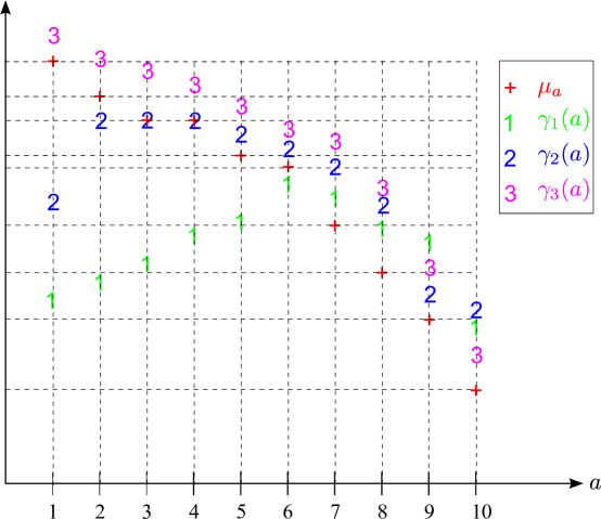
Figure 3: The pattern of $\gamma_{b}(a)$

We show an example in Figure 3, where $\mu_{1}\geq\cdots\geq\mu_{10}$. For $b=1$, $\gamma_{1}(1)<\cdots<\gamma_{1}(6)>\gamma_{1}(7)>\cdots>\gamma_{1}(10)$, $\gamma_{2}(a)<\mu_{a}$ for $a=1,\cdots,6$, and $\gamma_{2}(a)\geq\mu_{a}$ for $a=7,\cdots,10$. For $b=2$, $\gamma_{2}(1)<\gamma_{2}(2)=\gamma_{2}(3)=\gamma_{2}(4)>\cdots>\gamma_{2}(10)$, $\gamma_{2}(a)<\mu_{a}$ for $a=1,2$, and $\gamma_{2}(a)\geq\mu_{a}$ for $a=3,\cdots,10$. For $b=3$ $\gamma_{3}(1)>\cdots>\gamma_{3}(10)$, and $\gamma_{3}(a)\geq\mu_{a}$ for $a=1,\cdots,10$. Then we can verify the lemmas above and find that $l^{*}=6$, such that $\mu_{6}>g(\kern-0.24994pt\hbox{$\mu$}\kern-6.02548pt\kern 0.50003pt\hbox{$\mu$}\kern-6.02548pt\kern-0.24994pt\raise 0.43304pt\hbox{$\mu$},\kern-0.24994pt\hbox{$\nu$}\kern-4.93982pt\kern 0.50003pt\hbox{$\nu$}\kern-4.93982pt\kern-0.24994pt\raise 0.43304pt\hbox{$\nu$})=\gamma_{1}(6)\geq\mu_{7}$.

Since $\theta^{0}=\min\{\max_{a\in A}\delta_{a}^{0},g(\kern-0.24994pt\hbox{$\delta$}\kern-4.44444pt\kern 0.50003pt\hbox{$\delta$}\kern-4.44444pt\kern-0.24994pt\raise 0.43304pt\hbox{$\delta$}^{0},\kern-0.24994pt\hbox{$\sigma$}\kern-5.71413pt\kern 0.50003pt\hbox{$\sigma$}\kern-5.71413pt\kern-0.24994pt\raise 0.43304pt\hbox{$\sigma$}^{0})\}$, where $\kern-0.24994pt\hbox{$\delta$}\kern-4.44444pt\kern 0.50003pt\hbox{$\delta$}\kern-4.44444pt\kern-0.24994pt\raise 0.43304pt\hbox{$\delta$}^{0}=(\delta_{a}^{0})_{a\in A}$ and $\kern-0.24994pt\hbox{$\sigma$}\kern-5.71413pt\kern 0.50003pt\hbox{$\sigma$}\kern-5.71413pt\kern-0.24994pt\raise 0.43304pt\hbox{$\sigma$}^{0}=(\sigma_{b}^{0})_{b\in B}$, we have the following observations from Theorem 3.8:

1. When $C_{b}\sigma_{b}^{0}\geq\sum_{a\in A}C_{a\to b}\delta_{a}^{0}$ for all $b\in B$, then $g(\kern-0.24994pt\hbox{$\delta$}\kern-4.44444pt\kern 0.50003pt\hbox{$\delta$}\kern-4.44444pt\kern-0.24994pt\raise 0.43304pt\hbox{$\delta$}^{0},\kern-0.24994pt\hbox{$\sigma$}\kern-5.71413pt\kern 0.50003pt\hbox{$\sigma$}\kern-5.71413pt\kern-0.24994pt\raise 0.43304pt\hbox{$\sigma$}^{0})\geq\max_{a\in A}\delta_{a}^{0}$, and $\theta^{0}=\max_{a\in A}\delta_{a}^{0}$.

2. When $C_{b}\sigma_{b}^{0}<\sum_{a\in A}C_{a\to b}\delta_{a}^{0}$ for some $b\in B$, then there exists a unique, non-empty $A_{*}$ such that $\theta^{0}=g(\kern-0.24994pt\hbox{$\delta$}\kern-4.44444pt\kern 0.50003pt\hbox{$\delta$}\kern-4.44444pt\kern-0.24994pt\raise 0.43304pt\hbox{$\delta$}^{0},\kern-0.24994pt\hbox{$\sigma$}\kern-5.71413pt\kern 0.50003pt\hbox{$\sigma$}\kern-5.71413pt\kern-0.24994pt\raise 0.43304pt\hbox{$\sigma$}^{0})=\min_{b}\gamma_{b}(A_{*})$, and $\min_{a\in A_{*}}\delta_{a}^{0}>\theta^{0}\geq\max_{{\alpha}\in A\setminus A_{*}}\delta_{\alpha}^{0}$.

Thus $\theta^{0}$ is well-defined, bounded between $0$ and $\max_{a\in A}\delta_{a}^{0}$, and continuous in $(\delta_{1}^{0},\cdots,\delta_{m}^{0},\sigma_{m+1}^{0},\cdots,\sigma_{m+n}^{0})$.

4 Solutions to the Riemann problem

From the preceding section, we can see that the demand and supply levels satisfy the following conditions:

$$\{1=\delta^{0}_{a}=\delta^{*}_{a}\geq\delta_{a}>\tilde{\delta}_{a}\}\mbox{ or }\{\delta_{a}^{*}=\delta_{a}=\tilde{\delta}_{a}\mbox{ and }s_{a}^{0}\geq d_{a}\}$$ (21a)

$$\{1=\sigma^{0}_{b}=\sigma^{*}_{b}\geq\sigma_{b}>\tilde{\sigma}_{b}\}\mbox{ or }\{\sigma_{b}^{*}=\sigma_{b}=\tilde{\sigma}_{b}\mbox{ and }s_{b}^{0}\geq d_{b}\}$$ (21b)

$$\tilde{\delta}_{a}=\min\{\delta_{a}^{0},\theta^{0}\}$$ (21c)

$$\theta^{0}=\max_{a\in A}\delta_{a}^{0}\mbox{ or }(\delta_{a}^{0})_{a\in A_{*}\neq\emptyset}>\theta^{0}=\min_{b\in B}\gamma_{b}^{0}(A_{*})\geq(\delta_{a}^{0})_{a\in A\setminus A_{*}}$$ (21d)

$$C_{b}\tilde{\sigma}_{b}=\sum_{a\in A}C_{a\to b}\tilde{\delta}_{a}$$ (21e)

where $\gamma_{b}^{0}(A_{*})=\frac{C_{b}\sigma^{0}_{b}-\sum_{{\alpha}\in A\setminus A_{*}}C_{{\alpha}\to b}\delta_{\alpha}^{0}}{\sum_{a\in A_{*}}C_{a\to b}}$. In this section, we attempt to solve $\tilde{\delta}_{a}$ ($a\in A$) in $\delta_{a}$ and $\sigma_{b}$; i.e., a mapping from upstream demand levels and downstream supply levels to upstream flux levels:

$$(\tilde{\delta}_{1},\cdots,\tilde{\delta}_{m}) = {\mathbb{FF}}^{\prime}(\delta_{1},\cdots,\delta_{m},\sigma_{m+1},\cdots,\sigma_{m+n}).$$ (22)

Then from the definition of $\tilde{\delta}_{a}$ and (14c) we can have the flux function $(f_{1},\cdots,f_{m+n})={\mathbb{FF}}(d_{1},\cdots,d_{m},s_{m+1},\cdots,s_{m+n})$ and the corresponding Riemann solver.

4.1 Further properties of demand and supply levels

From Corollary 3.3 and (21) we have the following lemma.

Lemma 4.1

$U_{a}^{*}$ is SOC if and only if $\theta^{0}=\tilde{\delta}_{a}<\delta_{a}$, and $U_{a}^{*}$ is UC if and only if $\theta^{0}\geq\delta_{a}$. In addition, if $\theta^{0}<\delta_{a}$, then $U_{a}^{*}=U_{a}^{0}=(C_{a},f_{a})$ is SOC, and

$$1=\delta^{0}_{a}=\delta^{*}_{a}\geq\delta_{a}>\tilde{\delta}_{a}=\theta^{0};$$

if $\theta^{0}>\delta_{a}$, then $U_{a}^{*}=U_{a}^{0}=(d_{a},C_{a})$ is SUC, and

$$\delta^{0}_{a}=\delta^{*}_{a}=\delta_{a}=\tilde{\delta}_{a}<\theta^{0};$$

if $\theta^{0}=\delta_{a}$, then $U_{a}^{*}=(d_{a},C_{a})$ is UC, $U_{a}^{0}=(d_{a}^{0},s_{a}^{0})$ with $d_{a}^{0}\geq d_{a}$ and $s_{a}^{0}\geq d_{a}$, and

$$\delta^{0}_{a}\geq\delta^{*}_{a}=\delta_{a}=\tilde{\delta}_{a}=\theta^{0}.$$

In the third case, $U_{a}^{0}=U_{a}^{*}$ if and only if $\delta^{0}_{a}=\theta^{0}$, and the interior state $U_{a}^{0}$ is different from the stationary state $U_{a}^{*}$ when $\delta^{0}_{a}>\theta^{0}$.

An example of the relationships between $\delta_{a}$, $\delta_{a}^{*}$, $\delta^{0}_{a}$, and $\theta^{0}$ is shown in Figure 4, in which $U_{a}^{*}=U_{a}^{0}$ is SOC for $a=1,\cdots,4$, $U_{a}^{*}=U_{a}^{0}$ is UC for $a=6,\cdots,10$, and $U_{5}^{*}$ is UC but $U_{5}^{*}\neq U_{5}^{0}$.

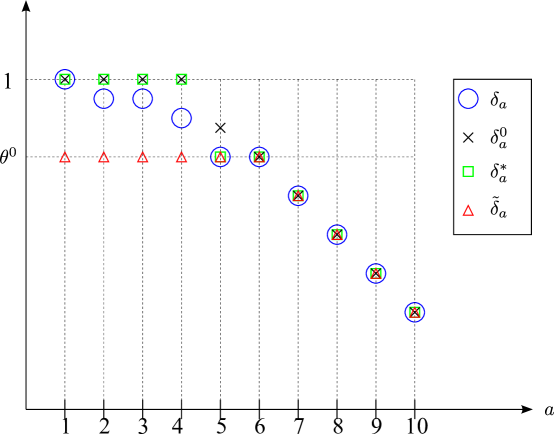
Figure 4: The relationships between $\delta_{a}$, $\delta^{*}_{a}$, $\delta^{0}_{a}$, $\tilde{\delta}_{a}$, and $\theta^{0}$

We define $A_{*}^{0}=\{a\in A|\delta^{0}_{a}>\theta^{0}\}$. From Lemma 4.1, $U_{a}^{*}$ is either SOC or UC with $U_{a}^{*}\neq U_{a}^{0}$ for $a\in A_{*}^{0}$; and $d_{\alpha}^{0}=d_{\alpha}$ for ${\alpha}\in A\setminus A_{*}^{0}$. From Theorem 3.8, we can see that $\min_{b\in B}\pi_{b}^{0}=\min_{b\in B}s_{b}^{0}-\sum_{a=1}^{m}C_{a\to b}\delta^{0}_{a}\geq 0$ iff $A_{*}^{0}$ is empty. If $A_{*}^{0}$ is non-empty, then $(\delta_{a}^{0})_{a\in A_{*}^{0}}>\theta^{0}=\min_{b\in B}\gamma^{0}_{b}(A_{*}^{0})\geq(\delta_{\alpha}^{0})_{{\alpha}\in A\setminus A_{*}^{0}}$. Then we have the following lemma.

Lemma 4.2

For downstream link $b$, if $A_{*}^{0}\neq\emptyset$ and $\gamma^{0}_{b}(A_{*}^{0})=\theta^{0}$ or if $A_{*}^{0}=\emptyset$ and $\pi_{b}^{0}=0$, then $U_{b}^{*}=U_{b}^{0}=(C_{b},s_{b})$ is OC, and

$$\sigma^{0}_{b}=\sigma^{*}_{b}=\sigma_{b}=\tilde{\sigma}_{b};$$

When $A_{*}^{0}\neq\emptyset$ and $\gamma^{0}_{b}(A_{*}^{0})>\theta^{0}$ or when $A_{*}^{0}=\emptyset$ and $\pi_{b}^{0}>0$, there can be two types of solutions: (i) $U_{b}^{*}=U_{b}^{0}=(f_{b},C_{b})$ is SUC, and

$$1=\sigma^{0}_{b}=\sigma^{*}_{b}\geq\sigma_{b}>\tilde{\sigma}_{b};$$

(ii) if $f_{b}=s_{b}<C_{b}$, another possible solution is that $U_{b}^{*}=(C_{b},s_{b})$ is SOC, $U_{b}^{0}=(d_{b}^{0},s_{b}^{0})\neq U_{b}^{*}$ with $d_{b}^{0}\geq s_{b}$ and $s_{b}^{0}>s_{b}$, and

$$\sigma^{0}_{b}>\sigma^{*}_{b}=\sigma_{b}=\tilde{\sigma}_{b}.$$

Therefore, if $U_{b}^{*}$ is SUC, $A_{*}^{0}=\emptyset$ and $\pi_{b}^{0}>0$ or $A_{*}^{0}\neq\emptyset$ and $\gamma^{0}_{b}(A_{*}^{0})>\theta^{0}$; if $U_{b}^{*}$ is OC, the interior state may not be the same as the stationary state. In addition, for all $b$, $\tilde{\sigma}_{b}\leq\sigma_{b}\leq\sigma_{b}^{*}\leq\sigma_{b}^{0}$, where all the equality signs hold when $A_{*}^{0}=\emptyset$ and $s_{b}^{0}=\sum_{a\in A}C_{a\to b}\delta^{0}_{a}$, or when $A_{*}^{0}\neq\emptyset$ and $\theta^{0}=\gamma^{0}_{b}(A_{*}^{0})$.

Proof.

1. When $A_{*}^{0}\neq\emptyset$ and $\gamma^{0}_{b}(A_{*}^{0})=\theta^{0}$, then from (14c) we have

   $$f_{b} = \theta^{0}\sum_{a\in A_{*}^{0}}C_{a\to b}+\sum_{{\alpha}\in A\setminus A_{*}^{0}}C_{{\alpha}\to b}\delta^{0}({\alpha})$$

   $$= \frac{s_{b}^{0}-\sum_{{\alpha}\in A\setminus A_{*}^{0}}C_{{\alpha}\to b}\delta^{0}({\alpha})}{\sum_{a\in A_{*}^{0}}C_{a\to b}}\sum_{a\in A_{*}^{0}}C_{a\to b}+\sum_{{\alpha}\in A\setminus A_{*}^{0}}C_{{\alpha}\to b}\delta^{0}({\alpha})=s_{b}^{0},$$

   If $f_{b}<s_{b}$; i.e., $U_{b}^{*}=U_{b}^{0}=(f_{b},C_{b})$ is SUC, and from (14c) we have $f_{b}=s_{b}^{0}=C_{b}<s_{b}$, which is impossible. Thus $f_{b}=s_{b}=s_{b}^{0}$, and $U_{b}^{*}=U_{b}^{0}=(C_{b},s_{b})$ is OC.

2. When $A_{*}^{0}=\emptyset$ and $\pi_{b}^{0}=0$, then from (14c) we have $f_{b}=s_{b}^{0}$. Similarly, we have $f_{b}=s_{b}=s_{b}^{0}$, and $U_{b}^{*}=U_{b}^{0}=(C_{b},s_{b})$ is OC.

3. When $A_{*}^{0}\neq\emptyset$ and $\gamma^{0}_{b}(A_{*}^{0})>\theta^{0}$, then from (14c) we have $f_{b}<s_{b}^{0}$. If $f_{b}<s_{b}$; i.e., $U_{b}^{*}=U_{b}^{0}=(f_{b},C_{b})$ is SUC, then $s_{b}^{0}=s_{b}^{*}=C_{b}\geq s_{b}>f_{b}$, and $1=\sigma^{0}_{b}=\sigma^{*}_{b}\geq\sigma_{b}>\tilde{\sigma}_{b}$. If $f_{b}=s_{b}$; i.e., $U_{b}^{*}=(C_{b},s_{b})$ is OC, and $U_{b}^{0}=(d_{b}^{0},s_{b}^{0})\neq U_{b}^{*}$ with $d_{b}^{0}\geq s_{b}$ and $s_{b}^{0}>s_{b}$, which is possible only if $s_{b}<C_{b}$. In this case, $\sigma^{0}_{b}>\sigma^{*}_{b}=\sigma_{b}=\tilde{\sigma}_{b}$.

4. When $A_{*}^{0}=\emptyset$ and $\pi_{b}^{0}>0$, similarly, there are two types of solutions: $U_{b}^{*}=U_{b}^{0}=(f_{b},C_{b})$ is SUC, then $s_{b}^{0}=s_{b}^{*}=C_{b}\geq s_{b}>f_{b}$, and $1=\sigma^{0}_{b}=\sigma^{*}_{b}\geq\sigma_{b}>\tilde{\sigma}_{b}$; $U_{b}^{*}=(C_{b},s_{b})$ is OC, $U_{b}^{0}=(d_{b}^{0},s_{b}^{0})\neq U_{b}^{*}$ with $d_{b}^{0}\geq s_{b}$ and $s_{b}^{0}>s_{b}$, which is possible only if $s_{b}<C_{b}$, and $\sigma^{0}_{b}>\sigma^{*}_{b}=\sigma_{b}=\tilde{\sigma}_{b}$.

$\blacksquare$

4.2 Solutions of the flux function

In addition to the interior critical demand function $\theta^{0}$ in (14b), we also define three other critical demand functions as follows:

$$\theta = \min\{\max_{a\in A}\delta_{a},\min_{b}\max_{A_{1}}\frac{s_{b}-\sum_{{\alpha}\in A\setminus A_{1}}d_{\alpha}\xi_{{\alpha}\to b}}{\sum_{a\in A_{1}}C_{a}\xi_{a\to b}}\}=\min\{\max_{a\in A}\delta_{a},g(\kern-0.24994pt\hbox{$\delta$}\kern-4.44444pt\kern 0.50003pt\hbox{$\delta$}\kern-4.44444pt\kern-0.24994pt\raise 0.43304pt\hbox{$\delta$},\kern-0.24994pt\hbox{$\sigma$}\kern-5.71413pt\kern 0.50003pt\hbox{$\sigma$}\kern-5.71413pt\kern-0.24994pt\raise 0.43304pt\hbox{$\sigma$})\},$$

$$\theta^{*} = \min\{\max_{a\in A}\delta_{a}^{*},\min_{b}\max_{A_{1}}\frac{s_{b}^{*}-\sum_{{\alpha}\in A\setminus A_{1}}d_{\alpha}^{*}\xi_{{\alpha}\to b}}{\sum_{a\in A_{1}}C_{a}\xi_{a\to b}}\}=\min\{\max_{a\in A}\delta_{a}^{*},g(\kern-0.24994pt\hbox{$\delta$}\kern-4.44444pt\kern 0.50003pt\hbox{$\delta$}\kern-4.44444pt\kern-0.24994pt\raise 0.43304pt\hbox{$\delta$}^{*},\kern-0.24994pt\hbox{$\sigma$}\kern-5.71413pt\kern 0.50003pt\hbox{$\sigma$}\kern-5.71413pt\kern-0.24994pt\raise 0.43304pt\hbox{$\sigma$}^{*})\},$$

$$\tilde{\theta} = \min\{\max_{a\in A}\tilde{\delta}_{a},\min_{b}\max_{A_{1}}\frac{s_{b}-\sum_{{\alpha}\in A\setminus A_{1}}f_{\alpha}\xi_{{\alpha}\to b}}{\sum_{a\in A_{1}}C_{a}\xi_{a\to b}}\}=\min\{\max_{a\in A}\tilde{\delta}_{a},g(\tilde{\kern-0.24994pt\hbox{$\delta$}\kern-4.44444pt\kern 0.50003pt\hbox{$\delta$}\kern-4.44444pt\kern-0.24994pt\raise 0.43304pt\hbox{$\delta$}},\kern-0.24994pt\hbox{$\sigma$}\kern-5.71413pt\kern 0.50003pt\hbox{$\sigma$}\kern-5.71413pt\kern-0.24994pt\raise 0.43304pt\hbox{$\sigma$})\}.$$

We define the residue supply of link $b$ by $\pi_{b}=s_{b}-\sum_{a=1}^{m}d_{a}\xi_{a\to b}$.

In the following, we demonstrate that there exists a global flux function, (12), satisfying (9), (10), and (14). We also show that the local flux function in (14) is invariant.

Theorem 4.3

For the Riemann problem, we have

$$\theta^{0} = \theta=\theta^{*}=\tilde{\theta},$$ (23)

$$\tilde{\delta}_{a} = \min\{\delta_{a},\theta\}=\min\{\delta_{a}^{0},\theta^{0}\}=\min\{\delta_{a}^{*},\theta^{*}\}=\min\{\delta_{a},\tilde{\theta}\}.$$ (24)

Therefore, the discrete flux function (14) is invariant.

Proof. First, if $\min_{b}\pi_{b}\geq 0$, all upstream links are stationary at UC; i.e., $q_{a}=d_{a}$ for $a\in A$. Otherwise, from Lemma 4.1 we have that $\theta^{0}<\max_{a}\delta_{a}\leq\max_{a}\delta_{a}^{0}$, and $A_{*}=\{a|\delta^{0}_{a}>\theta^{0}\}$ is not empty. From Theorem 3.8, there exists $b$, such that $\gamma_{b}^{0}(A_{*})=\theta^{0}$. Further from Lemma 4.2 we have that $f_{b}=s_{b}$. However, from (14c) we have the following contradiction:

$$f_{b} = \sum_{a\in A_{*}}\theta^{0}C_{a}+\sum_{{\alpha}\in A\setminus A_{*}}d_{\alpha}\xi_{{\alpha}\to b}<\sum_{a\in A}d_{a}\xi_{a\to b}\leq s_{b},$$

since $\theta^{0}<\max_{a}\delta_{a}$ and $\pi_{b}\geq 0$. Thus, no upstream links can have SOC stationary states, and from Lemma 4.1 we have that either $\delta_{a}^{0}=\delta_{a}^{*}=\delta_{a}=\tilde{\delta}_{a}<\theta^{0}$ or $\delta_{a}^{0}\geq\delta_{a}^{*}=\delta_{a}=\tilde{\delta}_{a}=\theta^{0}$ for any $a\in A$. Thus when $A_{*}=\{a|\delta^{0}_{a}>\theta^{0}\}$ is not empty, then $\theta^{0}=\max_{a\in A}\delta_{a}=\max_{a\in A}\delta_{a}^{*}=\max_{a\in A}\tilde{\delta}_{a}<\max_{a\in A}\delta_{a}^{0}$ ; otherwise, $\theta^{0}=\max_{a\in A}\delta_{a}=\max_{a\in A}\delta_{a}^{*}=\max_{a\in A}\tilde{\delta}_{a}=\max_{a\in A}\delta_{a}^{0}$. In addition, since $s_{b}^{*}\geq s_{b}\geq f_{b}$, $s_{b}^{*}-\sum_{a=1}^{m}d_{a}^{0}\xi_{a\to b}\geq 0$, and $s_{b}-\sum_{a=1}^{m}f_{a}\xi_{a\to b}$. From Theorem 3.8, $\theta=\max_{a\in A}\delta_{a}$, $\theta^{*}=\max_{a\in A}\delta_{a}^{*}$, and $\tilde{\theta}=\max_{a\in A}\tilde{\delta}_{a}$. Therefore, $\theta=\theta^{*}=\theta^{0}=\tilde{\theta}$, and $\tilde{\delta}_{a}=\min\{\delta_{a},\theta\}=\min\{\delta_{a}^{*},\theta^{*}\}=\min\{\delta_{a}^{0},\theta^{0}\}=\min\{\tilde{\delta}_{a},\tilde{\theta}\}$.

Second, if $\min_{b}\pi_{b}<0$, then at least one upstream has a SOC stationary state. Otherwise, $f_{a}=d_{a}$ for all $a$, from (14c) we have that $f_{b}=\sum_{a\in A}d_{a}\xi_{a\to b}>s_{b}$ when $\pi_{b}<0$. This contradicts $f_{b}\leq s_{b}$ for all $b$. From Lemma 4.1, $A_{*}^{0}=\{a|\theta^{0}<\delta^{0}_{a}\}$ is not empty. Thus $\tilde{\delta}_{a}=\theta^{0}$ for $a\in A_{*}$, and $\delta_{\alpha}^{0}=\delta_{\alpha}=\tilde{\delta}_{\alpha}=\delta_{\alpha}^{*}$ for ${\alpha}\in A\setminus A_{*}^{0}$. From Theorem 3.8, we have $\min_{a\in A_{*}^{0}}\delta^{0}_{a}>\theta^{0}=\min_{b\in B}\gamma_{b}^{0}(A_{*}^{0})\geq\max_{{\alpha}\in A\setminus A_{*}^{0}}\delta^{0}_{\alpha}$, where

$$\gamma_{b}^{0}(A_{*}^{0}) = \frac{s_{b}^{0}-\sum_{{\alpha}\in A\setminus A_{*}^{0}}C_{{\alpha}\to b}\delta_{\alpha}^{0}}{\sum_{a\in A_{*}^{0}}C_{a\to b}}=\frac{C_{b}\sigma_{b}^{0}-\sum_{{\alpha}\in A\setminus A_{*}^{0}}C_{{\alpha}\to b}\delta_{\alpha}}{\sum_{a\in A_{*}^{0}}C_{a\to b}}.$$

In addition,

$$\gamma_{b}(A_{*}^{0}) = \frac{C_{b}\sigma_{b}-\sum_{{\alpha}\in A\setminus A_{*}^{0}}C_{{\alpha}\to b}\delta_{\alpha}}{\sum_{a\in A_{*}^{0}}C_{a\to b}},$$

$$\gamma_{b}^{*}(A_{*}^{0}) = \frac{s_{b}^{*}-\sum_{{\alpha}\in A\setminus A_{*}^{0}}C_{{\alpha}\to b}\delta^{*}_{\alpha}}{\sum_{a\in A_{*}^{0}}C_{a\to b}}=\frac{C_{b}\sigma_{b}^{*}-\sum_{{\alpha}\in A\setminus A_{*}^{0}}C_{{\alpha}\to b}\delta_{\alpha}}{\sum_{a\in A_{*}^{0}}C_{a\to b}},$$

$$\tilde{\gamma}_{b}(A_{*}^{0}) = \frac{s_{b}-\sum_{{\alpha}\in A\setminus A_{*}^{0}}C_{{\alpha}\to b}\tilde{\delta}_{\alpha}}{\sum_{a\in A_{*}^{0}}C_{a\to b}}=\frac{C_{b}\sigma_{b}-\sum_{{\alpha}\in A\setminus A_{*}^{0}}C_{{\alpha}\to b}\delta_{\alpha}}{\sum_{a\in A_{*}^{0}}C_{a\to b}}.$$

From Lemma 4.2, there exists $b$ such that $\gamma_{b}^{0}(A_{*}^{0})=\theta^{0}$, for which $\sigma_{b}^{0}=\sigma_{b}^{*}=\sigma_{b}=\tilde{\sigma}_{b}$, and $\theta^{0}=\gamma_{b}(A_{*}^{0})=\tilde{\gamma}_{b}(A_{*}^{0})=\gamma_{b}^{*}(A_{*}^{0})$; for other $b\in B$, we have that $\gamma_{b}^{0}(A_{*}^{0})>\theta^{0}$, and $f_{b}=\theta^{0}\sum_{a\in A_{*}^{0}}C_{a\to b}+\sum_{{\alpha}\in A\setminus A_{*}^{0}}C_{{\alpha}\to b}\delta_{\alpha}\leq s_{b}\leq s_{b}^{*}$, which leads to $\theta^{0}\leq\gamma_{b}(A_{*}^{0})=\tilde{\gamma}_{b}(A_{*}^{0})\leq\gamma_{b}^{*}(A_{*}^{0})$. Thus we have

$$\min_{b\in B}\gamma_{b}(A_{*}^{0})=\min_{b\in B}\gamma_{b}^{*}(A_{*}^{0})=\min_{b\in B}\tilde{\gamma}_{b}(A_{*}^{0})=\min_{b\in B}\gamma_{b}^{0}(A_{*}^{0})=\theta^{0}.$$

If we denote $A_{*}=\{a|\theta^{0}<\delta_{a}\}$, which is the set of upstream links with SOC stationary states, then $A_{*}$ is not empty. From Lemma 4.1, we have that $A_{*}\subseteq A_{*}^{0}$ and $\theta^{0}=\tilde{\delta}_{a}=\delta_{a}=\delta^{*}_{a}<\delta^{0}_{a}$ for ${\alpha}\in A_{*}^{0}\setminus A_{*}$, which is the set of all upstream links with interior states. From Lemma 4.1, $\gamma_{b}(A_{*})=\gamma_{b}^{*}(A_{*})=\theta^{0}$ when $\gamma_{b}(A_{*}^{0})=\gamma_{b}^{*}(A_{*}^{0})=\theta^{0}$; and $\gamma_{b}(A_{*})=\gamma_{b}^{*}(A_{*})$ when $\gamma_{b}(A_{*}^{0})=\gamma_{b}^{*}(A_{*}^{0})>\theta^{0}$. Therefore, $\min_{b\in B}\gamma_{b}(A_{*})=\min_{b\in B}\gamma_{b}^{*}(A_{*})=\theta^{0}$. From Lemma 4.1 we have that $\theta^{0}<\delta_{a}\leq\delta^{*}_{a}$ for $a\in A_{*}$, and $\theta^{0}\geq\delta_{\alpha}=\delta^{*}_{\alpha}$ for ${\alpha}\in A\setminus A_{*}$. Thus we have $\min_{a\in A_{*}}\delta_{a}^{*}\geq\min_{a\in A_{*}}\delta_{a}>\min_{b\in B}\gamma_{b}(A_{*})=\min_{b\in B}\gamma_{b}^{*}(A_{*})=\theta^{0}\geq\max_{{\alpha}\in A\setminus A_{*}}\delta_{\alpha}=\max_{{\alpha}\in A\setminus A_{*}}\delta_{\alpha}^{*}$, which leads to $\min_{b\in B}\gamma_{b}(A_{*})=\theta=\theta^{*}=\theta^{0}$ from Theorem 3.8. Since $s_{b}\geq f_{b}=\sum_{a=1}^{m}C_{a\to b}\tilde{\delta}_{a}$, we have from Theorem 3.8 that $\tilde{\theta}=\max_{a\in A}\tilde{\delta}_{a}=\theta^{0}$ since $A_{*}^{0}$ is non-empty. In addition, when ${\alpha}\in A\setminus A_{*}^{0}$, $\theta^{0}\geq\delta_{\alpha}^{0}=\delta_{\alpha}=\delta_{\alpha}^{*}=\tilde{\theta}_{\alpha}$; when $a\in A_{*}^{0}$, $\theta^{0}\leq\delta_{a}\leq\delta_{a}^{*}\leq\delta_{a}^{0}$. In both cases, (24) is satisfied. $\blacksquare$

Remark. Note that Theorem 4.3 is also true when we switch the min and max operators in definitions of $\theta$, $\theta^{0}$, $\theta^{*}$, and $\tilde{\theta}$. From the proof of Theorem 3.8, we can see that these values remain the same when $\min_{b}\pi_{b}<0$. But if $\min_{b}\pi_{b}\geq 0$, the min-max and max-min operators could yield different values, which are not smaller than $\max_{a}\delta(a)$. A counter example is as follows: $d=[0.5,0.5]$, $C=[1,1]$, $\pi={{\left[\begin{array}[]{c}0.2\\ 0.2\end{array}\right]}}$, $\xi={{\left[\begin{array}[]{cc}0.8&0.2\\ 0.2&0.8\end{array}\right]}}$, then $\gamma={{\left[\begin{array}[]{ccc}0.75&1.5&0.7\\ 1.5&0.75&0.7\end{array}\right]}}$. In this case, $\min_{b}\max_{A_{1}}\gamma_{b}(A_{1})=1.5$, and $\max_{A_{1}}\min_{b}\gamma_{b}(A_{1})=0.75$. But both values are greater than 0.5, the maximum demand level. Thus Theorem 4.3 still holds.

Remark. From Theorem 4.3, we can find a unique flux function $(f_{1},\cdots,f_{m+n})={\mathbb{FF}}(d_{1},\cdots,d_{m},s_{m+1},\cdots,s_{m+n})$ defined in (12) and solve the Riemann problem in the following steps:

1. Calculate $\theta$ from initial conditions in $d_{a}$, $s_{b}$, and $\xi_{a\to b}$.

2. Calculate $f_{a}=\min\{d_{a},\theta C_{a}\}$, and $f_{b}=\sum_{a\in A}f_{a}\xi_{a\to b}$.

3. Determine stationary states and interior states from Corollary 3.2.

If we denote $\Theta=g(\kern-0.24994pt\hbox{$\delta$}\kern-4.44444pt\kern 0.50003pt\hbox{$\delta$}\kern-4.44444pt\kern-0.24994pt\raise 0.43304pt\hbox{$\delta$},\kern-0.24994pt\hbox{$\sigma$}\kern-5.71413pt\kern 0.50003pt\hbox{$\sigma$}\kern-5.71413pt\kern-0.24994pt\raise 0.43304pt\hbox{$\sigma$})$, then $\Theta=\theta$ when $\min_{b\in B}\pi_{b}<0$, and $\Theta\geq\theta$ when $\min_{b\in B}\pi_{b}\geq 0$. We can see that $f_{a}=\min\{d_{a},\Theta C_{a}\}$. We define $s_{a}^{+}=\Theta C_{a}$. Then $q_{a}=\min\{d_{a},s_{a}^{+}\}$, and $s_{a}^{+}$ can be considered as effective downstream supply of upstream link $a$. We define $\Theta_{-b}$ by $\theta_{-b}=\min_{{\beta}\in B\setminus\{b\}}\max_{A_{1}\subseteq A}\gamma_{\beta}(A_{1})$. Obviously $\Theta_{-b}\geq\Theta$. We have the following lemma.

Lemma 4.4

The in-flux of downstream link $b$ can be written as

$$f_{b} = \min\{d_{b}^{-},s_{b}\},$$

where

$$d_{b}^{-} = \sum_{a\in A}\min\{d_{a},\Theta_{-b}C_{a}\}\xi_{a\to b}.$$

That is, $d_{b}^{-}$ can be considered as effective upstream demand of downstream link $b$.

Proof. When $\min_{b\in B}\pi_{b}\geq 0$, from Theorem 3.8 we have that $\Theta\geq\max_{a\in A}\delta_{a}$, and $\Theta_{-b}\geq\max_{a\in A}\delta_{a}$. Thus $d_{b}^{-}=\sum_{a\in A}d_{a}\xi_{a\to b}\leq s_{b}$ since $\pi_{b}\geq 0$. From Theorem 4.3 we have $f_{b}=d_{b}^{-}=\min\{d_{b}^{-},s_{b}\}$.

When $\min_{b\in B}\pi_{b}<0$, if $\Theta_{-b}=\Theta$, then $f_{b}=d_{b}^{-}=\sum_{a\in A}f_{a}\xi_{a\to b}\leq s_{b}$; if $\Theta_{-b}>\Theta$, then from Theorem 3.8 there exists $A_{*}\neq\emptyset$ such that $\gamma_{b}(A_{*})=\Theta$ and $\min_{a\in A_{*}}\delta_{a}>\Theta\geq\max_{{\alpha}\in A\setminus A_{*}}\delta_{a}$. Therefore,

$$s_{b} = \Theta\sum_{a\in A_{*}}C_{a}\xi_{a\to b}+\sum_{{\alpha}\in A\setminus A_{*}}d_{\alpha}\xi_{{\alpha}\to b}=\sum_{a\in A}\min\{d_{a},\Theta C_{a}\}\xi_{a\to b}=f_{b}.$$

In addition, we have

$$f_{b} = \sum_{a\in A}\min\{d_{a},\Theta C_{a}\}\xi_{a\to b}\leq\sum_{a\in A}\min\{d_{a},\Theta_{-b}C_{a}\}\xi_{a\to b}=d_{b}^{-}.$$

Therefore, $f_{b}=\min\{d_{b}^{-},s_{b}\}$. $\blacksquare$

From Theorem 4.3 and Lemma 4.1, we have the following corollary.

Corollary 4.5

$U_{a}^{*}$ is SOC if and only if $d_{a}<s_{a}^{+}$, and $U_{a}^{*}$ is UC if and only if $d_{a}\geq s_{a}^{+}$. In addition, if $d_{a}>s_{a}^{+}$, then $U_{a}^{*}=U_{a}^{0}=(C_{a},q_{a})$ is SOC, and

$$1=\delta^{0}_{a}=\delta^{*}_{a}\geq\delta_{a}>\tilde{\delta}_{a}=\theta;$$

if $d_{a}<s_{a}^{+}$, then $U_{a}^{*}=U_{a}^{0}=(d_{a},C_{a})$ is UC, and

$$\delta^{0}_{a}=\delta^{*}_{a}=\delta_{a}=\tilde{\delta}_{a}<\theta;$$

if $d_{a}=s_{a}^{+}$, then $U_{a}^{*}=(d_{a},C_{a})$ is UC, $U_{a}^{0}=(d_{a}^{0},s_{a}^{0})$ with $d_{a}^{0}\geq d_{a}$ and $s_{a}^{0}\geq d_{a}$, and

$$\delta^{0}_{a}\geq\delta^{*}_{a}=\delta_{a}=\tilde{\delta}_{a}=\theta.$$

In the third case, it is possible that $U_{a}^{0}\neq U_{a}^{*}$, but $U_{a}^{0}=U_{a}^{*}$ is also a valid solution when $\delta_{a}^{0}=\delta_{a}$.

Similarly, from Theorem 4.3, Lemma 4.2, and Lemma 4.4 we have the following corollary regarding downstream links.

Corollary 4.6

$U_{b}^{*}$ is SUC if and only if $s_{b}>d_{b}^{-}$, and $U_{b}^{*}$ is OC if and only if $s_{b}\leq d_{b}^{-}$. In addition, if $s_{b}>d_{b}^{-}$, then $U_{b}^{*}=U_{b}^{0}=(q_{b},C_{b})$ is SUC, and

$$1=\sigma^{0}_{b}=\sigma^{*}_{b}\geq\sigma_{b}>\tilde{\sigma}_{b};$$

if $s_{b}<d_{b}^{-}$, then $U_{b}^{*}=U_{b}^{0}=(s_{b},C_{b})$ is OC, and

$$\sigma^{0}_{b}=\sigma^{*}_{b}=\sigma_{b}=\tilde{\sigma}_{b};$$

if $s_{b}=d_{b}^{-}$, then $U_{b}^{*}=(s_{b},C_{b})$ is OC, $U_{b}^{0}=(s_{b}^{0},s_{b}^{0})$ with $s_{b}^{0}\geq s_{b}$ and $s_{b}^{0}\geq s_{b}$, and

$$\sigma^{0}_{b}\geq\sigma^{*}_{b}=\sigma_{b}=\tilde{\sigma}_{b}.$$

In the third case, is is possible that $U_{b}^{0}\neq U_{b}^{*}$, but $U_{b}^{0}=U_{b}^{*}$ is also a valid solution when $\sigma^{0}_{b}=\sigma_{b}$.

5 Discussions

5.1 Special cases

For a linear junction with $m=n=1$, $\xi_{1\to 2}=1$, and $f_{1}=f_{2}$. In this case, $\Theta=\frac{s_{2}}{C_{1}}$, $\theta=\min\{\delta_{1},\frac{s_{2}}{C_{1}}\}$, and $f_{1}=\min\{\theta,\delta_{1}\}=\min\{\Theta,\delta_{1}\}$. Thus the effective supply of link 1 is $s_{1}^{+}=\Theta C_{1}=s_{2}$, and the effective demand of link 2 is $d_{2}^{-}=\min\{d_{1},\Theta_{-2}C_{1}\}=d_{1}$. From Theorem 4.3 we have $f_{1}=f_{2}=\min\{d_{1},s_{2}\}$. Thus from Corollaries 4.5 and 4.6 we have the following three cases.

1. When $s_{2}>d_{1}$, $d_{1}<s_{1}^{+}$, and $s_{2}>d_{2}^{-}$. Thus $U_{1}^{*}=U_{1}^{0}=(d_{1},C_{1})$ is UC, and $U_{2}^{*}=U_{2}^{0}=(d_{1},C_{2})$ is SUC. In this case, there is no interior state on either link.

2. When $s_{2}<d_{1}$, $d_{1}>s_{1}^{+}$, and $s_{2}<d_{s}^{-}$. Thus $U_{1}^{*}=U_{1}^{0}=(C_{1},s_{2})$ is SOC, and $U_{2}^{*}=U_{2}^{0}=(C_{2},s_{2})$ is OC. In this case, there is no interior state on either link.

3. When $s_{2}=d_{1}$, $d_{1}=s_{1}^{+}$, and $s_{2}=d_{s}^{-}$. Thus, $U_{1}^{*}=(d_{1},C_{1})$ is UC, and $U_{2}^{*}=(C_{2},s_{2})$ is OC. In this case, there can be interior states on both links: $U_{1}^{0}=(d_{1}^{0},s_{1}^{0})$, where $d_{1}^{0}\geq d_{1}$, and $s_{1}^{0}\geq d_{1}$; $U_{2}^{0}=(d_{2}^{0},s_{2}^{0})$, where $d_{2}^{0}\geq s_{2}$, and $s_{2}^{0}\geq s_{2}$. However, since $f_{1}=\min\{d_{1}^{0},s_{1}^{0}\}$, we have either $d_{1}^{0}=d_{1}$ or $s_{2}^{0}=s_{2}$. Thus $U_{1}^{0}=U_{1}^{*}$ or $U_{2}^{*}=U_{2}^{*}$; i.e., there can be only one interior state.

For a merging junction with $m>1$ and $n=1$, $\xi_{a\to m+1}=1$, and

$$\Theta = \max_{A_{1}\subset A}\frac{s_{m+1}-\sum_{{\alpha}\in A\setminus A_{1}}d_{\alpha}}{\sum_{a\in A_{1}}C_{a}}.$$

Thus the effective downstream supply for link $a\in A$ is $s_{a}^{+}=\Theta C_{a}$, and the effective upstream demand for link $m+1$ is $d_{m+1}^{-}=\sum_{a\in A}d_{a}$, since $\Theta_{-b}=1$. Then we can solve for stationary and interior states by following Corollaries 4.5 and 4.6. In particular, when $m=2$, we have

$$\Theta = \max\{\frac{s_{3}-d_{2}}{C_{1}},\frac{s_{3}-d_{1}}{C_{2}},\frac{s_{3}}{C_{1}+C_{2}}\},$$

$$q_{1} = \min\{d_{1},\Theta C_{1}\},$$

$$q_{2} = \min\{d_{2},\Theta C_{2}\},$$

which is consistent with the fair merge model in [28]:

$$q_{1} = \min\{d_{1},\max\{s_{3}-d_{2},\frac{C_{1}}{C_{1}+C_{2}}s_{3}\}\},$$

$$q_{2} = \min\{d_{2},\max\{s_{3}-d_{1},\frac{C_{2}}{C_{1}+C_{2}}s_{3}\}\}.$$

For a diverging junction with $m=1$ and $n>1$,

$$\Theta = \min_{b=2}^{1+n}\frac{s_{b}}{C_{1}\xi_{1\to b}}.$$

Thus the effective downstream supply for link 1 is $s_{1}^{+}=\Theta C_{1}=\min_{b=2}^{1+n}\frac{s_{b}}{\xi_{1\to b}}$, and the effective upstream demand for link $b\in B$ is $d_{b}^{-}=\min\{d_{1},\min_{{\beta}=2,{\beta}\neq b}^{n+1}\frac{s_{\beta}}{C_{1}\xi_{1\to{\beta}}}\}\xi_{1\to b}$. Then we can solve for stationary and interior states by following Corollaries 4.5 and 4.6. In particular,

$$q_{1} = \min\{d_{1},\Theta C_{1}\}=\min\{d_{1},\min_{b=2}^{1+n}\frac{s_{b}}{\xi_{1\to b}}\},$$

which is consistent with the FIFO diverge model [27].

For a junction with $m=2$ and $n=2$, we have

$$\Theta = \min\{\max\{\frac{s_{4}-d_{2}\xi_{2\to 4}}{C_{1}\xi_{1\to 4}},\frac{s_{4}-d_{1}\xi_{1\to 4}}{C_{2}\xi_{2\to 4}},\frac{s_{4}}{C_{1}\xi_{1\to 4}+C_{2}\xi_{2\to 4}}\},$$

$$\max\{\frac{s_{4}-d_{2}\xi_{2\to 4}}{C_{1}\xi_{1\to 4}},\frac{s_{4}-d_{1}\xi_{1\to 4}}{C_{2}\xi_{2\to 4}},\frac{s_{4}}{C_{1}\xi_{1\to 4}+C_{2}\xi_{2\to 4}}\}\},$$

$$f_{1} = \min\{d_{1},\Theta C_{1}\},$$

$$f_{2} = \min\{d_{2},\Theta C_{2}\}.$$

From Theorem 3.8, we can see that there are the following scenarios:

1. Both links 1 and 2 are stationary at UC if and only if $\Theta\geq\max\{\frac{d_{1}}{C_{1}},\frac{d_{2}}{C_{2}}\}$.

2. Link 1 is stationary at SOC and link 2 at UC if and only if $\frac{d_{1}}{C_{1}}>\Theta\geq\frac{d_{2}}{C_{2}}$.

3. Both links 1 and 2 are stationary at SOC if and only if $\Theta<\max\{\frac{d_{1}}{C_{1}},\frac{d_{2}}{C_{2}}\}$.

We can find all stationary and interior states by following Corollaries 4.5 and 4.6.

5.2 A simplified framework without interior states

Within the framework defined in Section 3.1 and a flux function in interior states in (14), the Riemann solver is well-defined since fluxes can be calculated from Theorem 4.3, and stationary and interior states can be determined from Corollaries 4.5 and 4.6.

From Corollaries 4.5 and 4.6, interior states can be the same as stationary states in all scenarios, and we can introduce a simplified framework as follows:

1. Stationary states arise near the junction on all links and satisfy (9).

2. An entropy condition is defined by the flux function in stationary states:

   $$\theta^{*} = \min\{\max_{a\in A}\delta_{a}^{*},g(\kern-0.24994pt\hbox{$\delta$}\kern-4.44444pt\kern 0.50003pt\hbox{$\delta$}\kern-4.44444pt\kern-0.24994pt\raise 0.43304pt\hbox{$\delta$}^{*},\kern-0.24994pt\hbox{$\sigma$}\kern-5.71413pt\kern 0.50003pt\hbox{$\sigma$}\kern-5.71413pt\kern-0.24994pt\raise 0.43304pt\hbox{$\sigma$}^{*})\},$$

   $$f_{a} = \min\{d_{a}^{*},\theta^{*}C_{a}\},\forall a\in A$$

   $$f_{b} = \sum_{a\in A}f_{a}\xi_{a\to b},\forall b\in B$$

From Theorem 4.3, the Riemann problem is uniquely solved and the out-flux of upstream link $a$ is still given by $f_{a}=\min\{d_{a},\theta C_{a}\}$. Further, Corollaries 4.5 and 4.6 can be used to determine unique stationary states.

Note that, however, not all CTM flux functions can be used in the simplified framework. For example, with the following flux function proposed in [32]

$$f_{a} = \min\{d_{a}^{0},\min_{b\in B}\frac{d_{a}^{0}}{\sum_{{\alpha}\in A}d_{\alpha}^{0}\xi_{a\to b}}s_{b}^{0}\},$$ (25a)

$$f_{b} = \sum_{a\in A}f_{a}\xi_{a\to b},$$ (25b)

it was shown that $f_{a}=\min\{d_{a},\theta C_{a}\}$, but it is possible that interior states are different from stationary states. In this case, ${\mathbb{FF}}^{0}(d_{1}^{0},\cdots,d_{m}^{0},s_{m+1}^{0},\cdots,s_{m+n}^{0})={\mathbb{FF}}(d_{1},\cdots,d_{m},s_{m+1},\cdots,s_{m+n})={\mathbb{FF}}^{*}(d_{1}^{*},\cdots,d_{m}^{*},s_{m+1}^{*},\cdots,s_{m+n}^{*})$, but

$${\mathbb{FF}}^{0}(d_{1}^{0},\cdots,d_{m}^{0},s_{m+1}^{0},\cdots,s_{m+n}^{0})\neq{\mathbb{FF}}(d_{1}^{0},\cdots,d_{m}^{0},s_{m+1}^{0},\cdots,s_{m+n}^{0}).$$

That is, ${\mathbb{FF}}^{0}(\cdots)\neq{\mathbb{FF}}(\cdots)$, and it is not invariant. Therefore, with an invariant flux function, the network kinematic wave model (1) can be defined in the function space of traditional weak solutions. But for a non-invariant flux function, e.g., (25), the function space has to be extended to include interior states.

Clearly we have that

$${\mathbb{RS}}({\mathbb{RS}}(k_{1},\cdots,k_{m+n}))={\mathbb{RS}}(k_{1},\cdots,k_{m+n}).$$

That is, the Riemann solver is consistent in the sense of [15]. In addition, all Godunov flux functions can be used as entropy conditions in the simplified framework, in which interior states are the same as stationary states.

5.3 A stationary junction network

A junction network is stationary if and only if all initial states are the same as stationary states; i.e., $U_{a}=U_{a}^{*}$ for $a\in A$, and $U_{b}=U_{b}^{*}$ for $b\in B$. From Corollaries 4.5 and 4.6, it is possible that $d_{a}=d_{a}^{*}$ ($a\in A$) and $s_{b}=s_{b}^{*}$ ($b\in B$). Therefore, such stationary states always exist. In addition, if $U_{a}$ and $U_{b}$ are stationary, then

$$f_{a} = \min\{d_{a},\Theta C_{a}\}=\min\{d_{a},s_{a}\},$$

$$f_{b} = \min\{d_{b}^{-},s_{b}\}=\min\{d_{b},s_{b}\}.$$

From Corollary 4.5 we can see that, if $U_{a}=(C_{a},s_{a})$ is SOC, then $\Theta C_{a}=s_{a}=q_{a}$; if $U_{a}=(d_{a},C_{a})$ is UC, then $\Theta\geq\delta_{a}$. From Corollary 4.6 we can see that, if $U_{b}=(d_{b},C_{b})$ is SUC, $d_{b}^{-}=q_{b}<C_{b}$; if $U_{b}=(C_{b},s_{b})$ is OC, then $d_{b}^{-}\geq s_{b}$.

When a junction network is stationary, we can replace any SOC state $(C_{a},\theta C_{a})$ by the corresponding SUC state $(\theta C_{a},C_{a})$, and $\theta$ remains the same; but we may not replace a SUC state by the corresponding SOC state. Thus for the same fluxes, there can be multiple combinations of stationary states. Furthermore, if we replace $d_{a}$ by $q_{a}=\theta C_{a}$ for $a\in A_{*}$, then all upstream links will be stationary at UC, and the critical demand level and all upstream flow-rates remain unchanged. In addition, if all upstream links are stationary at UC, we can replace an OC stationary state on link $b$, $(C_{b},q_{b})$, by an UC state, $(q_{b},C_{b})$.

6 Conclusion

The kinematic wave model of network traffic flow, (1), is thus well-defined by the following rules.

• The constitutional law: $q_{a}(x_{a},t)=k_{a}(x_{a},t)v_{a}(x_{a},t)$ at any point $x_{a}$ on link $a$ and time $t$.

• The fundamental diagram of speed-density relation, $v_{a}(x_{a},t)=V_{a}(k(x_{a},t))$, flow-density relation, $q_{a}(x_{a},t)=Q_{a}(k(x_{a},t))\equiv k_{a}(x_{a},t)V_{a}(k_{a}(x_{a},t))$, demand-density relation, $d_{a}(x_{a},t)=Q_{a}(\min\{k_{a,c},k_{a}(x_{a},t)\})$, and supply-density relation, $s_{a}(x_{a},t)=Q_{a}(\max\{k_{a,c},k_{a}(x_{a},t)\})$.

• Traffic conservation: ${\frac{\partial{k_{a}}}{\partial{t}}}+{\frac{\partial{q_{a}}}{\partial{x_{a}}}}=0$.

• Weak solutions with interior states: the kinematic wave model can have discontinuous weak solutions and interior states at stationary discontinuities.

• Entropy conditions with local flux functions at any junction at $x$: we denote the set of upstream demands by ${\bf d}(x^{-},t)$ and the set of downstream supplies by ${\bf s}(x^{+},t)$, then the set of boundary fluxes ${\bf f}(x,t)={\mathbb{FF}}^{0}({\bf d}(x^{-},t),{\bf s}(x^{+},t))$.

Thus, if initial conditions in densities and boundary conditions in demands at origins and supplies at destinations are given, (1) can be uniquely solved with the aforementioned five rules.

This modeling framework makes the entropy condition explicit by using boundary flux functions. In a sense, it is the reverse process of Godunov method, in which flux functions were derived by solving Riemann problems with entropy conditions defined in characteristics or other approaches [33]. It is possible to extend this framework for more complicated situations for multi-class traffic on multi-lane roads or for other types of intersections. The challenges will be related to identifying fundamental diagrams and developing boundary flux functions. Therefore, the Riemann solver can be used to determine whether a flux function is well-defined both mathematically and physically.

In addition, it is possible to extend this framework to study other systems of hyperbolic conservation laws, in which demand and supply functions are well-defined. For example, numerical E-O flux function and other approximate Riemann solvers can be used as entropy conditions when solving the Burgers equation.

In the future, we will be interested in analyzing traffic dynamics in a road network with the help of the new kinematic wave model. Such a Riemann solver and the corresponding kinematic wave model can be used to study many other transportation network problems.

References

- [1] R. Ansorge. What does the entropy condition mean in traffic flow theory? Transportation Research Part B, 24(2):133–143, 1990.
- [2] A. Aw and M. Rascle. Resurrection of “second order” models of traffic flow. SIAM Journal on Applied Mathematics, 60(3):916–938, 2000.
- [3] H. Bar-Gera and S. Ahn. Empirical macroscopic evaluation of freeway merge-ratios. Transportation Research Part C, 18(4):457–470, 2010.
- [4] M. Beckmann. A continuous model of transportation. Econometrica: Journal of the Econometric Society, pages 643–660, 1952.
- [5] S. Benzoni-Gavage and R. Colombo. An n-populations model for traffic flow. European Journal of Applied Mathematics, 14(05):587–612, 2003.
- [6] A. Bressan and H. Jenssen. On the convergence of godunov scheme for nonlinear hyperbolic systems. Chinese Annals of Mathematics Series B, 21(3):269–284, 2000.
- [7] M. Bultelle, M. Grassin, and D. Serre. Unstable Godunov discrete profiles for steady shock waves. SIAM Journal on Numerical Analysis, 35(6):2272–2297, 1998.
- [8] M. Cassidy and S. Ahn. Driver turn-taking behavior in congested freeway merges. Transportation Research Record: Journal of the Transportation Research Board, 1934:140–147, 2005.
- [9] G. Coclite, M. Garavello, and B. Piccoli. Traffic flow on a road network. SIAM Journal on Mathematical Analysis, 36(6):1862–1886, 2005.
- [10] C. Daganzo. In traffic flow, cellular automata= kinematic waves. Transportation Research Part B, 40(5):396–403, 2006.
- [11] C. F. Daganzo. The cell transmission model II: Network traffic. Transportation Research Part B, 29(2):79–93, 1995.
- [12] C. F. Daganzo. The nature of freeway gridlock and how to prevent it. Proceedings of the 13th International Symposium on Transportation and Traffic Theory, pages 629–646, 1996.
- [13] C. F. Daganzo. A continuum theory of traffic dynamics for freeways with special lanes. Transportation Research Part B, 31(2):83–102, 1997.
- [14] B. Engquist and S. Osher. One-sided difference schemes and transonic flow. Proceedings of the National Academy of Sciences, 77(6):3071–3074, 1980.
- [15] M. Garavello. Conservation laws at a node. Nonlinear Conservation Laws and Applications, pages 293–302, 2011.
- [16] M. Garavello and B. Piccoli. Source-Destination flow on a road network. Communications in Mathematical Sciences, 3(3):261–283, 2005.
- [17] M. Garavello and B. Piccoli. Traffic flow on a road network using the Aw-Rascle model. Communications in Partial Differential Equations, 31(2):243–275, 2006.
- [18] D. C. Gazis, R. Herman, and R. W. Rothery. Nonlinear follow-the-leader models of traffic flow. Operations Research, 9(4):545–567, 1961.
- [19] S. K. Godunov. A difference method for numerical calculations of discontinuous solutions of the equations of hydrodynamics. Matematicheskii Sbornik, 47(3):271–306, 1959. In Russian.
- [20] B. D. Greenshields. A study in highway capacity. Highway Research Board Proceedings, 14:448–477, 1935.
- [21] B. Haut and G. Bastin. A second order model of road junctions in fluid models of traffic networks. Networks and Heterogeneous Media, 2(2):227, 2007.
- [22] M. Herty, C. Kirchner, S. Moutari, and M. Rascle. Multicommodity flows on road networks. Communications in Mathematical Sciences, 6(1):171–187, 2008.
- [23] M. Herty, S. Moutari, and M. Rascle. Optimization criteria for modelling intersections of vehicular traffic flow. Networks and Heterogeneous Media, 1(2):275–294, 2006.
- [24] H. Ho and S. Wong. Two-dimensional continuum modeling approach to transportation problems. Journal of Transportation Systems Engineering and Information Technology, 6(6):53–68, 2006.
- [25] H. Holden and N. H. Risebro. A mathematical model of traffic flow on a network of unidirectional roads. SIAM Journal on Mathematical Analysis, 26(4):999–1017, 1995.
- [26] W.-L. Jin. Asymptotic traffic dynamics arising in diverge-merge networks with two intermediate links. Transportation Research Part B, 43(5):575–595, 2009.
- [27] W.-L. Jin. Analysis of kinematic waves arising in diverging traffic flow models. Arxiv preprint, 2010.
- [28] W.-L. Jin. Continuous kinematic wave models of merging traffic flow. Transportation Research Part B, 44(8-9):1084–1103, 2010.
- [29] W.-L. Jin. A kinematic wave theory of multi-commodity network traffic flow. Transportation Research Part B, 2012. in press.
- [30] W.-L. Jin, L. Chen, and E. G. Puckett. Supply-demand diagrams and a new framework for analyzing the inhomogeneous Lighthill-Whitham-Richards model. Proceedings of the 18th International Symposium on Transportation and Traffic Theory, pages 603–635, 2009.
- [31] W.-L. Jin and H. M. Zhang. The inhomogeneous kinematic wave traffic flow model as a resonant nonlinear system. Transportation Science, 37(3):294–311, 2003.
- [32] W.-L. Jin and H. M. Zhang. A multicommodity kinematic wave simulation model of network traffic flow. Transportation Research Record: Journal of the Transportation Research Board, 1883:59–67, 2004.
- [33] P. D. Lax. Hyperbolic systems of conservation laws and the mathematical theory of shock waves. SIAM, Philadelphia, Pennsylvania, 1972.
- [34] J. P. Lebacque. The Godunov scheme and what it means for first order traffic flow models. Proceedings of the 13th International Symposium on Transportation and Traffic Theory, pages 647–678, 1996.
- [35] J. P. Lebacque. Intersection modeling, application to macroscopic network traffic flow models and traffic management. In S. Hoogendorn, S. Luding, P. Bovy, M. Schreckenberg, and D. Wolf, editors, Traffic and Granular Flow ’03, pages 261–278. Springer, 2005.
- [36] R. J. LeVeque. Finite volume methods for hyperbolic problems. Cambridge University Press, Cambridge; New York, 2002.
- [37] M. J. Lighthill and G. B. Whitham. On kinematic waves: II. A theory of traffic flow on long crowded roads. Proceedings of the Royal Society of London A, 229(1178):317–345, 1955.
- [38] J. C. Muñoz and C. F. Daganzo. The bottleneck mechanism of a freeway diverge. Transportation Research Part A, 36(6):483–505, 2002.
- [39] K. Nagel and M. Schreckenberg. A cellular automaton model for freeway traffic. Journal de Physique I France, 2(2):2221–2229, 1992.
- [40] D. Ni and J. Leonard. A simplified kinematic wave model at a merge bottleneck. Applied Mathematical Modelling, 29(11):1054–1072, 2005.
- [41] M. Papageorgiou and A. Kotsialos. Freeway ramp metering: An overview. IEEE Transactions on Intelligent Transportation Systems, 3(4):271–281, 2002.
- [42] H. J. Payne. Models of freeway traffic and control. Simulation Councils Proceedings Series: Mathematical Models of Public Systems, 1(1):51–61, 1971.
- [43] P. I. Richards. Shock waves on the highway. Operations Research, 4(1):42–51, 1956.
- [44] P. Roe. Approximate riemann solvers, parameter vectors, and difference schemes. Journal of Computational Physics, 43(2):357–372, 1981.
- [45] D. Schrank and T. Lomax. The 2009 annual urban mobility report. Technical report, Texas Transportation Institute, The Texas A&M Universtiy, 2009.
- [46] Y. Sheffi, H. Mahmassani, and W. Powell. A transportation network evacuation model. Transportation Research Part A, 16(3):209–218, 1982.
- [47] B. van Leer. On the relation between the upwind-differencing schemes of Godunov, Engquist-Osher and Roe. SIAM Journal on Scientific and Statistical Computing, 5(1):1–20, 1984.
- [48] G. B. Whitham. Linear and nonlinear waves. John Wiley and Sons, New York, 1974.
- [49] J. Wu, Y. Chen, and M. Florian. The continuous dynamic network loading problem: A mathematical formulation and solution method. Transportation Research Part B, 32(3):173–187, 1998.
- [50] H. M. Zhang. A non-equilibrium traffic model devoid of gas-like behavior. Transportation Research Part B, 36(3):275–290, 2002.