Topological entropy and secondary folding

Abstract

A convenient measure of a map or flow’s chaotic action is the topological entropy. In many cases, the entropy has a homological origin: it is forced by the topology of the space. For example, in simple toral maps, the topological entropy is exactly equal to the growth induced by the map on the fundamental group of the torus. However, in many situations the numerically-computed topological entropy is greater than the bound implied by this action. We associate this gap between the bound and the true entropy with ‘secondary folding’: material lines undergo folding which is not homologically forced. We examine this phenomenon both for physical rod-stirring devices and toral linked twist maps, and show rigorously that for the latter secondary folds occur.

I Introduction

In many industrial applications, fluid is stirred by moving rods to achieve homogeneity. Such a simple system also serves as a testbed for ideas about mixing and transport barriers. In the past few years, a topological description of rod-stirring has emerged (see for example Boyland et al. (2000); Thiffeault and Finn (2006); Thiffeault and Pavliotis (2008); Finn and Thiffeault (2011)). In this framework, the two-dimensional fluid lives in a surface with holes, with the holes corresponding to moving rods and fixed baffles. This topological description applies to all fluids, but is most useful for very viscous flows.

A consequence of the topological description is that we can compute lower bounds on the topological entropy of the system. The topological entropy is, roughly speaking, the growth rate of material lines in a fluid Adler et al. (1965); Newhouse (1988). The lower bound on the topological entropy is a consequence of continuity – material lines cannot cross the rods, so they must grow at least as fast as dictated by the motion of the rods.

We can then ask about the sharpness of this lower bound: we measure the actual growth rate of material lines in the flow, and compare it to the lower bound. In many systems, the ‘gap’ between the lower bound and the actual value is quite small – on the order of a few percent of the value. In other cases, the gap is very large, so that the observed value of the entropy is much larger than the lower bound. The central question of this paper is: what accounts for the difference in these two cases? In both cases, much of the entropy is ‘homological’ and arises from obstructions in the domain – the rods and baffles. This homological entropy depends only weakly on the details of the physical system, and can be deduced without actually solving the dynamical fluid equations. However, in the cases with a large gap it seems clear that there is another, dynamical source of entropy, which can depend more strongly on system parameters, such as the size of the stirring rods and the fluid being considered. We propose that the so called dynamical entropy is predominately due to secondary folding, where material lines exhibit folds that are not directly associated with a topological obstacle.

When the difference between the bound and the measured entropy is small, we refer to those bounds as sharp. We will investigate the sharpness of the bound by considering simple three-rod stirring devices. The motion of the rods is limited to a sequence of clockwise or counter-clockwise exchanges with one of their neighbors, following circular paths Boyland et al. (2000). These types of motions map naturally to generators of the braid group Birman (1975): a clockwise exchange of the $i$th and $(i+1)$th rod is denoted $\sigma_{i}$, and a counter-clockwise exchange by $\sigma_{i}^{-1}$. A sequence of $\sigma_{i}^{\pm 1}$ is called a stirring protocol. Since the fluid we consider is highly viscous, the stirring protocols define a periodic motion of the fluid elements, obtained by solving Stokes’ equation for incompressible flow. Figure 1 shows some examples of stirring protocols, as well as their action on typical material lines.

We will illustrate the gap between the bound and measured value using two examples in Section II. Because the disk with three punctures (rods) has such an intimate connection with the torus, we will examine toral maps in Section III. We observe the same gap phenomenon as in the fluid case, but because the map is a much simpler system we are able to prove some explicit results about toral maps: in particular, we demonstrate the presence of secondary folds, or ‘kinks.’ Finally, in Section IV we summarize our results and discuss future work.

II Some Observations

As an illustration of the gap phenomenon in hydrodynamic flows, consider a stirring device with three rods that initially lie in a line. There are many ways to move the rods and stir the fluid, but we are primarily interested in the topological aspects of the motion. As discussed in the introduction, we focus on sequences of interchanges of neighboring rods, which we label by generators of the braid group Boyland et al. (2000); Thiffeault and Finn (2006). Here, we consider two stirring protocols, given in terms of generators by $\sigma_{1}\sigma_{2}^{-1}$ and $\sigma_{1}\sigma_{2}^{5}$, where generators are read left to right. The rod motions are depicted in the insets in Figure 1. The exact details of how we move the rods make no difference to the topology of the system, though it will in general affect the measured growth rate of material lines. The speed of motion is irrelevant, since we are in the Stokes flow regime. In the simulations below, we always use circular paths and constant speed.

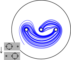
(a)   $\sigma_{1}\sigma_{2}^{-1}$

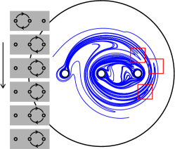
(b)   $\sigma_{1}\sigma_{2}^{5}$

Figure 1: The effect of two different stirring protocols on the same initial material line. The insets show the motion of the rods. The images are after four and three periods, respectively. In (b) boxes highlight some instances of secondary folding. There is no secondary folding visible in (a).

II.1 Computing $h_{\text{hom}}$ and $h_{\text{flow}}$

Two types of topological entropy will be computed here. The first, called $h_{\text{hom}}$, is the entropy coming from the homology, i.e. the entropy due to the rod motion alone. This is the lower bound alluded to in the introduction: it is the growth rate of a hypothetical ‘rubber band’ caught on the rods, and is independent of both the type of fluid being stirred and the specifics of the rod motion. This entropy is computed directly from the braid describing the rod motion. The second entropy we compute, $h_{\text{flow}}$, is obtained by directly measuring the growth rate of material lines in the flow. We have $h_{\text{hom}}\leq h_{\text{flow}}$, since material lines cannot (asymptotically) grow slower than the minimum rate dictated by the rods. We now discuss how to compute $h_{\text{hom}}$ and $h_{\text{flow}}$.

Computing $h_{\text{hom}}$ can be difficult when dealing with a large number of rods or long sequences of generators, though rapid techniques have been developed Moussafir (2006); Thiffeault (2010). However, for three rods the entropy is very easy to compute. In that case, the topological entropy is equal to logarithm of the spectral radius (largest magnitude over all eigenvalues) of the Burau representation matrix Burau (1936); Fried (1986); Kolev (1989); Boyland et al. (2003); Band and Boyland (2007). For braids of the form $\sigma_{1}^{\ell}\sigma_{2}^{-k}$ the Burau matrix is

$$[\sigma_{1}^{k}\sigma_{2}^{-\ell}]=\begin{bmatrix}1+k\ell&\ell\\ k&1\end{bmatrix}.$$ (1)

If $h_{\text{hom}}>0$, then, under repeated iterations, a rubber band caught on the rods will grow in length at an exponential rate. In this case, the braid is called pseudo-Anosov. If $h_{\text{hom}}=0$, the rubber band will not grow exponentially, and the braid is said to be finite-order. This terminology comes from the Thurston–Nielsen theory of classification of surface homeomorphisms Fathi et al. (1979); Thurston (1988). There is a third case in the classification, called reducible, which is not relevant here. Mixers with pseudo-Anosov stirring protocols are usually good at mixing; the exponential stretching and folding of material lines leads to a growth in the interface between solutes, which in turn allows diffusion or chemical reaction to act more rapidly.

Now for $h_{\text{flow}}$: in theory it is computed by taking the supremum of growth rates over all material lines in the fluid Newhouse (1988). In practice, a typical material line will eventually grow at a maximal rate, as long as some part of it is in the ergodic component with the fastest growth rate. Thus, we can get a good measure of $h_{\text{flow}}$ for each protocol by computing the rate at which a typical material line stretches. We do this by solving numerically for the motion of the individual fluid elements making up a material line, taking care to interpolate new points as the distance between neighbors becomes too large.

II.2 Stirring Protocol $\sigma_{1}\sigma_{2}^{-1}$ vs. $\sigma_{1}\sigma_{2}^{5}$

We compare two stirring protocols, given in braid form by $\sigma_{1}\sigma_{2}^{-1}$ and $\sigma_{1}\sigma_{2}^{5}$. Using the matrix (1), we find that they both have $h_{\text{hom}}=\log((3+\sqrt{5})/2)\simeq 0.962$. Despite this, the effect on material lines is quite different, as can be see by comparing Figures 1(a) and 1(b). Notice that for the $\sigma_{1}\sigma_{2}^{-1}$ protocol (Fig. 1(a)) the material line forms very smooth and regular layers; the only large visible folds are due to wrapping around the rods. On the other hand, for the $\sigma_{1}\sigma_{2}^{5}$ protocol (Fig. 1(b)), the material line has extra folds that are not due to wrapping around a rod, as highlighted by the boxes. These are what we call ‘secondary folds.’

From simulations we can measure $h_{\text{flow}}$ for each stirring protocol. Figure 2 shows the measured length of a material line during several periods of the flow. The length is plotted on a log scale, and the (asymptotic) slope of the line is $h_{\text{flow}}$. In this way, we measure $h_{\text{flow}}=0.991$ for the $\sigma_{1}\sigma_{2}^{-1}$ protocol, and $h_{\text{flow}}=1.61$ for the $\sigma_{1}\sigma_{2}^{5}$ protocol. For $\sigma_{1}\sigma_{2}^{-1}$, the rod entropy and the flow entropy agree well (roughly a 3% difference). However, for $\sigma_{1}\sigma_{2}^{5}$, the flow entropy is much larger than the rod entropy ($h_{\text{hom}}$ accounts for roughly $61\%$ of $h_{\text{flow}}$). We hypothesize that the larger measured entropy is due to additional stretching of the material line due to the secondary folds.

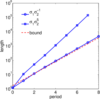
Figure 2: Growth of the length of a material line for the two stirring protocols. Since they are both pseudo-Anosov systems, the slope, i.e. the growth rate tends to a constant – namely the topological entropy. The dashed line has slope equal to the lower bound, $h_{\text{hom}}=0.962$.

III Toral Linked Twist Map

It is problematic to define secondary folding rigorously in a practical context, which also makes it difficult to identify its causes. To make headway, we look at a simpler system – a map instead of a hydrodynamic flow – which can be analyzed more thoroughly. The class of maps we’ll examine are toral linked twist maps. Linked twist maps (or LTMs) have been studied extensively Sturman et al. (2006); Przytycki (1983, 1986); Springham and Wiggins (2010); Donnay (1992); Devaney (1978, 1980); Burton and Easton (1980). They are non-uniformly hyperbolic, and are especially relevant here because of an intimate connection to the three-rod stirring protocols above. The connection arises through the orientable double cover Boyland et al. (2000); Farb and Margalit (2011): the torus can be regarded as a double cover of the disk with three punctures. The double cover branches at each of the punctures and at the disk’s outer boundary. The interchange of rods given by $\sigma_{1}$ and $\sigma_{2}$ in the three-rod system correspond to the vertical and horizontal Dehn twists in the toral LTM.

The domain of the toral LTM is an L-shaped subset of the flat torus formed by two overlapping orthogonal strips. One full application of the map consists of two consecutive linear shears. The first shear takes place in the vertical strip of width $\alpha$, and the second shear is in the horizontal strip of height $\beta$ (Figure 3). The integer parameters $k$ and $\ell$ are the strengths of each shear. In the limit $\alpha=\beta=1$, toral LTMs reduce to toral maps with uniform stretching. These are often called generalized Arnold cat maps: the cat map is the toral LTM with $\alpha=\beta=k=\ell=1$. Toral LTMs can also be defined more generally with non-linear shears Sturman et al. (2006), but we do not deal with those here. If $k\ell>0$ we say that the system is counter-rotating; if $k\ell<0$ we say that it is co-rotating. This naming convention is the opposite of the one used by some other authors, for instance Sturman et al. (2006). In the present context, given the rod-stirring applications, it is more natural to define co-rotating and counter-rotating as we do here.

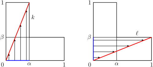
Figure 3: The toral LTM consists of two linear shears. The first shear (left image) is in a vertical strip on the torus. The left edge of the strip remains fixed, while the right edge is translated by $k$ units. The second shear (right image) is in a horizontal strip. The bottom edge remains fixed, while the top edge is translated by $\ell$ units. Here, the shears are shown with $k=\ell=1$.

Although we don’t have a true fluid flow here, we can still compare the topological entropy measured from the stretching rate of a material line to a lower bound for the topological entropy of the map. This lower bound arises from a semi-conjugacy between the toral LTM and the generalized Arnold cat map with the same $k$ and $\ell$ Franks (1970). The generalized Arnold cat map acts on the full torus with the same matrix given in (1). For $k$ and $\ell$ such that the matrix is hyperbolic, the topological entropy is again the log of the magnitude of the largest eigenvalue.

As a parallel to our $\sigma_{1}\sigma_{2}^{-1}$ and $\sigma_{1}\sigma_{2}^{5}$ examples above, we look at toral LTMs with $k=1$, $\ell=1$ (counter-rotating) and $k=1$, $\ell=-5$ (co-rotating). Figure 4 shows, for both the counter-rotating and co-rotating maps, the image of an initial line segment after two iterations. As with the hydrodynamic flow examples, they both have a lower bound of $h_{\text{hom}}=0.962$. Numerically measuring the stretching of the line yields $h_{\text{flow}}=0.962$ for the counter-rotating LTM and $h_{\text{flow}}=1.91$ for the co-rotating case. As for the three-rod mixers, the entropy agrees well with the lower bound for the counter-rotating example ($<1\%$ difference), but there is a large gap for the co-rotating example ($h_{\text{hom}}$ accounts for roughly $49.6\%$ of $h_{\text{flow}}$). Looking again at Figure 4, we notice visible secondary folding in the co-rotating case (indicated by boxes), but none in the counter-rotating case. This holds in general for toral LTMs. To prove this, we take a closer look at the toral LTM map.

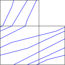
(a)  counter-rotating

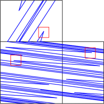
(b)  co-rotating

Figure 4: Images of the same initial line segment after two iterations for (a) a counter-rotating toral LTM ($k=\ell=1$), and (b) a co-rotating toral LTM ($k=1$, $\ell=5$). The small boxes highlight examples of secondary folding (acute angles) in the co-rotating case.

III.1 Secondary Folding in Toral LTMs

Recall that the toral LTM is the composition of a shear in a vertical strip of the torus and a shear in a horizontal strip on the torus. As a result, the domain is partitioned into three regions: points that undergo the vertical shear, but not the horizontal; points that undergo the horizontal shear, but not the vertical; and points that undergo both shears. We label these three regions $R_{V}$, $R_{H}$, and $R_{L}$ as follows (see Figure 5):

$$R_{V} =\{(x,y)\bmod 1\,|\,\,0\leq x\leq\alpha,\;\beta<y+xk\alpha^{-1}<1\};$$ (2a)

$$R_{H} =\{(x,y)\bmod 1\,|\,\,\alpha<x<1,\;0\leq y\leq\beta\};$$ (2b)

$$R_{L} =\{(x,y)\bmod 1\,|\,\,0\leq x\leq\alpha,\;0\leq y+xk\alpha^{-1}\leq\beta\},$$ (2c)

and also define $R=R_{V}\cup R_{H}\cup R_{L}$.

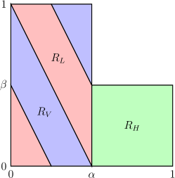
Figure 5: The three regions given by Equation (2), shown here with $k=1$.

More specifically, for a point $z=(x,y)^{\text{T}}$, the toral LTM map is given by

$$M(z)=\begin{cases}Vz\bmod{1},&\text{if $z\in R_{V}$};\\ Hz\bmod{1},&\text{if $z\in R_{H}$};\\ Lz\bmod{1},&\text{if $z\in R_{L}$},\end{cases}$$ (3)

where $V$, $H$, and $L$ are the matrices

$$V=\begin{bmatrix}1&0\\ \kappa&1\end{bmatrix},\quad H=\begin{bmatrix}1&\lambda\\ 0&1\end{bmatrix},\quad L=HV=\begin{bmatrix}1+\kappa\lambda&\lambda\\ \kappa&1\end{bmatrix},$$ (4)

with $\kappa=k\alpha^{-1}$ and $\lambda=\ell\beta^{-1}$. The toral LTM is continuous and piecewise linear.

Because of the piecewise nature of linear toral LTMs, the image of a line segment that crosses from one region to another will be a segmented line. This is the origin of all bends in iterates of line segments. Bends can be either obtuse or acute. We conjecture that obtuse bends do not contribute to the topological entropy, and so we ignore them; however, acute bends (also called kinks) always appear associated with an increased topological entropy. These kinks are the manifestation of secondary folds on the torus. To show the existence (or non-existence) of kinks, we examine the unstable manifold. This is sufficient since, under repeated iteration, a line segment will align with the unstable manifold and stretch in that direction.

A subtle but important point here is that there is a set of singularities, $\mathcal{S}\in R$, where the unstable (and stable) manifolds don’t exist Sturman et al. (2006); Wojtkowski (1980). This set consists of all points on the boundaries of the $R_{L}$, $R_{V}$, and $R_{H}$ regions, as well as all (forward and backward) images of these points. These singularities exist because the toral LTM is continuous, but not differentiable, on the boundaries of the regions, so the tangent vector is not well-defined at those points. (These singular points eventually become the vertices of bends in line segments.) Fortunately, $\mathcal{S}$ is a set of measure zero Wojtkowski (1980), and tangent vectors are well defined in the neighborhood of the singularities. So, using continuity, we will speak of having an ‘unstable’ manifold at each singular point, even though it may be the vertex of a bend. Then, since line segments tend to align with the unstable manifold, if a system has a kinked unstable manifold then any line segment will also develop kinks.

The following lemma gives the slope of the unstable manifold at any (non-singular) point.

Lemma 1.

For a toral LTM, the slope of the unstable manifold at a point $z\in R\setminus\mathcal{S}$ is given by

$$S_{u}(z)=\cfrac{1}{\lambda n_{1}+\cfrac{1}{\kappa m_{1}+\cfrac{1}{\lambda n_{2}+\cfrac{1}{\kappa m_{2}+\dots}}}}$$ (5)

where $m_{i},n_{i}>0$ if $z$ is in the horizontal strip, and $m_{i},n_{i}>0$ but $n_{1}=0$ otherwise. The $m_{i}$ and $n_{i}$ are unique integers that result from iterating $z$ backwards along its orbit.

(Note that this continued fraction was derived in a slightly different manner in Wojtkowski (1980).)

Proof.

We use the fact that under repeated forward iterations, all line segments converge to the unstable manifold. To approximate the unstable manifold at point $z$, we first follow $z$ backwards along its orbit to some point $z^{\prime}$. Then, we can take (almost) any vector in the tangent space, $T_{z^{\prime}}R=\mathbb{R}^{2}$, and map it forward to $z$. The image of the vector at $z$ will be approximately tangent to the unstable manifold at $z$. (This fails only when the initial vector is exactly aligned with the stable manifold.)

Each iteration of the inverse linked twist map, $M^{-1}(z)$, leads multiplication by either $V^{-1}$, $H^{-1}$, or $L^{-1}=V^{-1}H^{-1}$, depending on the location of $z$. So repeated backward iterations can be written as

$$z^{\prime}=M^{-N}(z)=V^{-m_{j}}H^{-n_{j}}\dots V^{-m_{1}}H^{-n_{1}}(z)$$ (6)

where $N=\sum_{i=1}^{j}(m_{i}+n_{i}-1)$. (The value of $j$ depends on both $N$ and $z$.) In general, $m_{i},n_{i}>0$. However, for some points, the first action of the inverse map is $V^{-1}$, not $H^{-1}$, so for these points, $n_{1}=0$. These are exactly the points that are not in the horizontal strip. (Additionally, for a given $N$ and $z$, we might have $m_{j}=0$. In this case, (9) below ends with $\lambda n_{j}$; this does not change the argument.)

Let $w^{\prime}$ be a vector in $T_{z^{\prime}}R=\mathbb{R}^{2}$. Since $DV=V$ and $DH=H$, $w$ and $z^{\prime}$ evolve according to exactly the same matrix multiplication. That is, $w\in T_{z}R$ can be written as

$$w=H^{n_{1}}V^{m_{1}}H^{n_{2}}V^{m_{2}}\dots H^{n_{j}}V^{m_{j}}w^{\prime}\,.$$ (7)

Now consider how multiplication by $H^{n}V^{m}$ affects the slope of a vector. If the vector initially has slope $s$, then after multiplication by $H^{n}V^{m}$ it has slope

$$s^{\prime}=\frac{s+\kappa m}{1+\lambda n(s+\kappa m)}=\cfrac{1}{\lambda n+\cfrac{1}{\kappa m+s}}\;.$$ (8)

Repeated iteration to find the slope at $w$ gives the finite continued fraction

$$\text{slope}(w)=\cfrac{1}{\lambda n_{1}+\cfrac{1}{\kappa m_{1}+\cfrac{1}{\lambda n_{2}+\cfrac{1}{\kappa m_{2}+\cfrac{1}{\dots+\cfrac{1}{\kappa m_{j}}}}}}}\;.$$ (9)

To find the exact slope, let $N~{}\rightarrow~{}\infty$. This means $j~{}\rightarrow~{}\infty$ and the finite continued fraction becomes the infinite continued fraction given in (5). So it only remains to show that the continued fraction converges. In the counter-rotating case, $\kappa\lambda>0$, and we have $\kappa m_{i}\geq 1$ and $\lambda n_{i}\geq 1$. Hence $\sum(\kappa m_{i}+\lambda n_{i})$ diverges, and the continued fraction converges to a finite value by the Seidel–Stern Theorem Jones and Thron (1980).

By definition, the co-rotating toral LTM must have $k\ell<0$, or equivalently $\kappa\lambda<0$. However, we add another restriction and require $\kappa\lambda<-4$. This condition ensures that matrix $L$ is hyperbolic and, consequently, that the toral LTM has an ergodic partition Wojtkowski (1980). (With a slightly stronger condition, the toral LTM will also be Bernoulli Przytycki (1983).) To show convergence in this case, we transform the continued fraction into the form

$$S_{u}(z)=\cfrac{(\lambda n_{1})^{-1}}{1+\cfrac{(\kappa\lambda m_{1}n_{1})^{-1}}{1+\cfrac{(\kappa\lambda m_{1}n_{2})^{-1}}{1+\cfrac{(\kappa\lambda m_{2}n_{2})^{-1}}{1+\dots}}}}\ .$$ (10)

Note that since $\kappa\lambda<-4$, each of the numerators (except for the first) has magnitude less than $1/4$. The continued fraction then converges to a finite value by Worpitzky’s Theorem Jones and Thron (1980). (The case where $n_{1}=0$ follows similarly.) ∎

We intend to show that counter-rotating toral LTMs do not have kinks, while co-rotating toral LTMs do. Therefore, we proceed by investigating each type separately. For convenience, we assume in both cases that $k>0$.

III.1.1 Counter-rotating

Since we are only considering maps with $k>0$, we have $\ell>0$ as well. Then every part of the continued fraction (5) is positive, and we conclude that the slope of the unstable manifold, $S_{u}$, is positive at every point $z\in R\setminus\mathcal{S}$. Furthermore, it is easy to show that the orientation of the unstable manifold is preserved under the action of the map.

Define two cones in tangent space $TR=\mathbb{R}^{2}$ by

$$C_{1} =\{(u,v)\,|\,\,u>0,v>0\},$$ (11)

$$C_{3} =\{(u,v)\,|\,\,u<0,v<0\}.$$ (12)

(The subscripts refer to the standard quadrant numbering.) Note that the definitions are independent of $z$.

Lemma 2.

For $k,\ell>0$, the cones $C_{1}$ and $C_{3}$ are invariant under both the vertical twist ($V$) and the horizontal twist ($H$).

Proof.

Take a vector $w=(u,v)$. Then $Vw=\left(u,v+u\kappa\right)$, and $Hw=\left(u+v\lambda,v\right)$. Clearly, if $w\in C_{1}$ then both $Vw$ and $Hw$ are also in $C_{1}$ (and therefore $Lw\in C_{1}$). Similarly, if $w\in C_{3}$ then both $Vw$ and $Hw$ are also in $C_{3}$. ∎

Corollary 3.

A line segment with positive slope will never kink under applications of $M$.

Proof.

Consider a line segment, $\gamma$, with positive slope passing through a point $z$. Let $w_{1}$ and $w_{3}$ be vectors in $T_{z}R$ that are tangent to $\gamma$ and such that $w_{1}\in C_{1}$ and $w_{3}\in C_{3}$. Then from Lemma 2, $DM(w_{1})\in C_{1}$ and $DM(w_{3})\in C_{3}$ regardless of which region $z$ is in. Consequently, the angle between the vectors is obtuse, and no kink has formed. ∎

Theorem 4.

The unstable manifold of a counter-rotating toral LTM has no kinks.

Proof.

Suppose that there is a kink in the unstable manifold. Then there must be a portion of the unstable manifold that is a straight line, crosses a region boundary, and maps to the kink. But $S_{u}>0$ for counter-rotating toral LTMs, which contradicts Corollary 3. Hence, there are no kinks in the unstable manifold. ∎

III.1.2 Co-rotating

Next we consider co-rotating toral LTM, and again restrict attention to ones with $k>0$ and $\kappa\lambda<-4$, so that the matrix $L$ is hyperbolic. For such toral LTMs, we prove that the unstable manifold is kinked.

We begin by using the eigenvectors of $L$ to define two pairwise-invariant cones (as in Sturman et al. (2006)). For each point $z\in R$, we define two cones in the tangent space $T_{z}R$ by

$$C(z) =\{(u,v)\,|\,\,m_{*}\leq v/u\leq 0\},$$ (13)

$$\widetilde{C}(z) =\{(u,v)\,|\,\,0<m_{*}+\kappa\leq v/u\},$$ (14)

where $m_{*}$ is the slope of the expanding eigenvector of $L$ and for co-rotating maps:

$$m_{*}=\frac{2\kappa}{\kappa\lambda-\sqrt{\kappa\lambda(\kappa\lambda+4)}}=-\frac{\kappa\lambda+\sqrt{\kappa\lambda(\kappa\lambda+4)}}{2\lambda}<0.$$ (15)

Note that cone definitions are independent of $z$, so we can refer to them simply as $C$ and $\widetilde{C}$. For convenience, we let $I_{C}=[m_{*},0]$ and $I_{\widetilde{C}}=[m_{*}+\kappa,\infty)$ denote the range of slopes in cones $C$ and $\widetilde{C}$ respectively. The following lemma shows that tangent vectors to the unstable manifold lie precisely in these cones.

Lemma 5.

For $\kappa\lambda<-4$ and $z\in R\setminus\mathcal{S}$, the slope of the unstable manifold, $S_{u}(z)$, lies in $C$ if $z$ is in the horizontal strip, and lies in $\widetilde{C}$ otherwise.

Proof.

This follows from a modification of a theorem by Hillam and Thron regarding convergence regions of continued fractions Hillam and Thron (1965). They look at a sequence of maps, $F_{i}=f_{1}\circ f_{2}\circ\cdots\circ f_{i}$, where $f_{i}$ has the form $f_{i}(\tau)={a_{i}}/{(b_{i}+\tau)}$, and the sequence $\{F_{i}(0)\}$ gives successive convergents of a continued fraction. They prove that if there exists a disk $D=\{w\in\mathbb{C}\,|\,\,|w-c|\leq r\}$, with $|c|<r$ and $f_{i}(D)\subseteq D$, then the continued fraction converges to a value in $D$.

We modify this proof for our purposes so that $f_{i}(\tau)$ has the form

$$f_{i}(\tau)=\cfrac{1}{\lambda n_{i}+\cfrac{1}{\kappa m_{i}+\tau}}\,.$$ (16)

Now the sequence $\{F_{i}(0)\}$ gives the even numbered convergents of the continued fraction (5). Since we know that the continued fraction converges (Lemma 1), these even numbered convergents will converge to the same value as the continued fraction.

The disk we use is $D=\{w\in\mathbb{C}\,|\,\,|w-m_{*}/2|\leq-m_{*}/2\}$. This is the smallest disk possible, because when $n_{i}=m_{i}=1$, $f_{i}(m_{*})=m_{*}$. To see that $f_{i}(D)\subseteq D$, re-write $f_{i}(\tau)$ as

$$f_{i}(\tau)=\frac{\tau+\kappa n_{i}}{\lambda n_{i}\tau+\kappa\lambda n_{i}m_{i}+1}$$ (17)

and view it as a Möbius transformation. Then $f_{i}(\partial D)$ is a circle with center and radius given by:

center $$=\frac{1}{2}\left(\frac{\kappa m_{i}}{1+\kappa\lambda m_{i}n_{i}}+\frac{m_{*}+\kappa m_{i}}{1+\lambda n_{i}(m_{*}+\kappa m_{i})}\right)$$ (18)

radius $$=\frac{m_{*}}{2(1+\kappa\lambda m_{i}n_{i})|1+\lambda n_{i}(m_{*}+\kappa m_{i})|}.$$ (19)

From these, it is easy to check that $f_{i}(D)\subseteq D$. The intersection of $D$ with the real axis is the interval $I_{C}=[m_{*},0]$, i.e. exactly the range of slopes in $C$. Thus, for $n_{i}>0$, $S_{u}(z)\in I_{C}$ and the unstable manifold is in $C$.

When $n_{1}=0$, equation (5) has the form

$$S_{u}(z)=\kappa m_{1}+\cfrac{1}{\lambda n_{2}+\cfrac{1}{\kappa m_{2}+\cfrac{1}{\lambda n_{3}+\dots}}}$$ (20)

and $S_{u}(z)\in I_{\widetilde{C}}$ follows in the same manner. ∎

The following lemma shows how a kink may be formed after one application of the toral LTM.

Lemma 6.

Take a point $z\in\mathcal{S}\subset R$ on the boundary between the $R_{L}$ and $R_{H}$ regions (i.e. $z\in R_{L}\cap\overline{R_{H}}$). Then a line segment passing through $z$ (possibly with a bend at $z$) and with the segments on either side of $z$ having slope $s\in(-\kappa-\lambda^{-1},0]$ will form an acute angle, with vertex at $M(z)$, after one application of $M$.

Proof.

Suppose for simplicity that $z$ is on the right-hand boundary of $R_{L}$, as in Figure 6. (The case where $z$ is on the left-hand boundary is proved in an identical manner.)

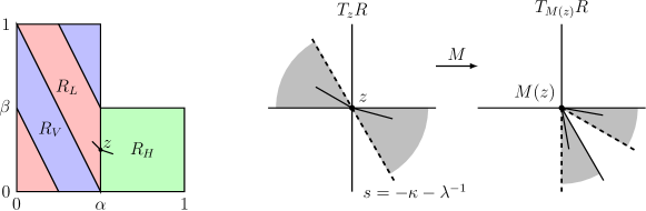
Figure 6: A (possibly jointed) line segment passing through a point on the boundary of $R_{L}$ and $R_{H}$, with slope $m\in(-\kappa-\lambda^{-1},0]$, will form a kink after one iteration of $M$.

The portion of the line segment that lies to the left of point $z$ is in the region $R_{L}$. Let $u=(u_{1},u_{2})$ be a vector that is parallel to the line segment and points left. That is, $u_{1}<0$ and, because $u_{2}/u_{1}\in(-\kappa-\lambda^{-1},0]$, we have $u_{2}\geq 0$. In this region the action of the toral LTM is multiplication by the matrix $L=HV$. So if the segment left of $z$ is initially parallel to $u$, then it will be parallel to $u^{\prime}=Lu$ after $M$ has been applied. We can compute $u^{\prime}=\left(u_{1}+u_{1}\kappa\lambda+u_{2}\lambda,u_{2}+u_{1}\kappa\right)$, and it is easy to see that $u^{\prime}$ points strictly into the 4th quadrant.

Meanwhile, the portion of the line segment that lies to the right of point $z$ is in the region $R_{H}$. Let $v=(v_{1},v_{2})$ be a vector that is parallel to the line segment and points right. That is, $v_{1}>0$ and $v_{2}\leq 0$. Since we are in region $R_{H}$, the action of the toral LTM is multiplication by the matrix $H$. So after $M$ is applied, the line segment will be parallel to $v^{\prime}=Hv$. Simple computation yields $v^{\prime}=\left(v_{1}+v_{2}\lambda,v_{2}\right)$, and we can see that $v^{\prime}$ points either horizontally or into the 4th quadrant. Thus, $M(z)$ is the vertex of an acute angle and a kink has formed. ∎

Theorem 7.

The unstable manifold of a co-rotating toral LTM with $\kappa\lambda<-4$ has kinks.

Proof.

Lemma 5 shows that for non-singular points in the horizontal strip, the unstable manifold is in cone $C$. Since $I_{C}\subset(-\kappa-\lambda^{-1},0]$, pieces of the unstable manifold that cross the boundaries between $R_{L}$ and $R_{H}$ satisfy the hypotheses of Lemma 6. Thus, these pieces kink after one application of $M$. Since pieces of unstable manifold map to other pieces of unstable manifold, this implies that there already existed kinks in the unstable manifold. ∎

IV Discussion

We set out to explain the gap between the homological lower bound on the topological entropy and its numerically-observed value. We observed that, in both fluid-dynamical systems and toral LTMs, the presence of a gap appeared associated with ‘secondary folding’ – the presence of extra folds in material lines, not associated with topological obstacles such as rods. Though we have not been able to rigorously show that the gap is due to the folds, we were able to show that counter-rotating toral LTMs never have folds, while hyperbolic co-rotating toral LTMs always have folds. This correlates perfectly with the presence or absence of a gap in the topological entropy. Future work will aim to show that secondary folding is the direct cause of the extra entropy.

References

- Boyland et al. (2000) P. L. Boyland, H. Aref, and M. A. Stremler, J. Fluid Mech. 403, 277 (2000).
- Thiffeault and Finn (2006) J.-L. Thiffeault and M. D. Finn, Philos. Trans. R. Soc. Lond. Ser. A Math. Phys. Eng. Sci. 364, 3251 (2006).
- Thiffeault and Pavliotis (2008) J.-L. Thiffeault and G. A. Pavliotis, Physica D 237, 918 (2008), arXiv:physics/0703135 .
- Finn and Thiffeault (2011) M. D. Finn and J.-L. Thiffeault, SIAM Rev. (2011), http://arXiv.org/abs/1004.0639 .
- Adler et al. (1965) R. L. Adler, A. G. Konheim, and M. H. McAndrew, Trans. Amer. Math. Soc. 114, 309 (1965).
- Newhouse (1988) S. E. Newhouse, Ergodic Theory Dynam. Systems 8∗, 283 (1988).
- Birman (1975) J. S. Birman, Braids, Links, and Mapping Class Groups, Annals of Mathematics Studies (Princeton University Press, Princeton, NJ, 1975).
- Moussafir (2006) J.-O. Moussafir, Func. Anal. and Other Math. 1, 37 (2006), arXiv:math.DS/0603355 .
- Thiffeault (2010) J.-L. Thiffeault, Chaos 20, 017516 (2010), arXiv:0906.3647 .
- Burau (1936) W. Burau, Abh. Math. Semin. Hamburg Univ. 11, 171 (1936).
- Fried (1986) D. Fried, Topology 25, 455 (1986).
- Kolev (1989) B. Kolev, C. R. Acad. Sci. Sér. I 309, 835 (1989), english translation at http://arxiv.org/abs/math.DS/0304105.
- Boyland et al. (2003) P. L. Boyland, M. A. Stremler, and H. Aref, Physica D 175, 69 (2003).
- Band and Boyland (2007) G. Band and P. Boyland, Algebr. Geom. Topol. 7, 1345 (2007).
- Birman and Brendle (2005) J. S. Birman and T. E. Brendle, in Handbook of Knot Theory, edited by W. Menasco and M. Thistlethwaite (Elsevier, Amsterdam, 2005) pp. 19–104, available at http://arXiv.org/abs/math.GT/0409205.
- Fathi et al. (1979) A. Fathi, F. Laundenbach, and V. Poénaru, Astérisque 66-67, 1 (1979).
- Thurston (1988) W. P. Thurston, Bull. Amer. Math. Soc. (N.S.) 19, 417 (1988).
- Sturman et al. (2006) R. Sturman, J. M. Ottino, and S. Wiggins, The Mathematical Foundations of Mixing: The Linked Twist Map as a Paradigm in Applications: Micro to Macro, Fluids to Solids (Cambridge University Press, Cambridge, U.K., 2006).
- Przytycki (1983) F. Przytycki, Ann. Sci. École Norm. Sup. (4) 16, 345 (1983).
- Przytycki (1986) F. Przytycki, Studia Math. 83, 1 (1986).
- Springham and Wiggins (2010) J. Springham and S. Wiggins, Dyn. Syst. 25, 483 (2010).
- Donnay (1992) V. J. Donnay, in Twist mappings and their applications, IMA Vol. Math. Appl., Vol. 44 (Springer, New York, 1992) pp. 95–117.
- Devaney (1978) R. L. Devaney, Proc. Amer. Math. Soc. 71, 334 (1978).
- Devaney (1980) R. L. Devaney, in Global theory of dynamical systems (Proc. Internat. Conf., Northwestern Univ., Evanston, Ill., 1979), Lecture Notes in Math., Vol. 819 (Springer, Berlin, 1980) pp. 121–145.
- Burton and Easton (1980) R. Burton and R. W. Easton, in Global theory of dynamical systems (Proc. Internat. Conf., Northwestern Univ., Evanston, Ill., 1979), Lecture Notes in Math., Vol. 819 (Springer, Berlin, 1980) pp. 35–49.
- Farb and Margalit (2011) B. Farb and D. Margalit, A Primer on Mapping Class Groups (Princeton University Press, Princeton, NJ, 2011).
- Franks (1970) J. Franks, in Global Analysis (Proc. Sympos. Pure Math., Vol. XIV, Berkeley, Calif., 1968) (Amer. Math. Soc., Providence, R.I., 1970) pp. 61–93.
- Wojtkowski (1980) M. Wojtkowski, in Nonlinear dynamics (Internat. Conf., New York, 1979), Ann. New York Acad. Sci., Vol. 357 (New York Acad. Sci., New York, 1980) pp. 65–76.
- Jones and Thron (1980) W. B. Jones and W. J. Thron, Continued Fractions: Analytic Theory and Applications, Encyclopedia of Mathematics and its Applications, Vol. 11 (Addison-Wesley, 1980).
- Hillam and Thron (1965) K. L. Hillam and W. J. Thron, Proc. Amer. Math. Soc. 16, 1256 (1965).