Modified Holographic Dark Energy in Non-flat Kaluza$-$Klein Universe with Varying $G$

Abstract

The purpose of this paper is to discuss the evolution of modified holographic dark energy with variable $G$ in non-flat Kaluza$-$Klein universe. We consider the non-interacting and interacting scenarios of the modified holographic dark energy with dark matter and obtain the equation of state parameter through logarithmic approach. It turns out that the universe remains in different dark energy eras for both cases. Further, we study the validity of the generalized second law of thermodynamics in this scenario. We also justify that the statefinder parameters satisfy the limit of $\Lambda$CDM model.

Keywords: Kaluza$-$Klein cosmology; Modified holographic dark energy; Dark matter; Generalized second law of thermodynamics.
PACS: 04.50.Cd; 95.36.+d; 95.35.+x; 98.80.-k

1 Introduction

The discovery of the accelerating expansion of the universe is a milestone for cosmology which has deep implications for the composition of the universe, structure formation and its fate. The expansion of the universe shows that it is not slowing down under normal gravity but accelerating due to an unknown component termed as dark energy (DE), having a strong negative pressure [1]. There are many pieces of evidence for the existence of this component of the universe other than the baryonic and non-baryonic dark matter (DM) [2] but it has no clear clue about its identity.

The most convenient explanation for this expansion is the vacuum energy that generates sufficient force to push matter apart described by cosmological constant [2]. However, there are two alternative ways used extensively in order to explain this behavior. The first approach is the work on different DE models such as quintessence [3], K-essence [4], phantom [5], quintom [6], tachyon [7], family of Chaplygin gas [8], holographic [9, 10] and new agegraphic DE [11]. Among all these models, holographic DE models are widely used. They provide the link of the DE density to the cosmic horizon [12] and has been tested through various astronomical observations [13].

The idea of holographic DE model (HDE) can be extracted from the holographic principle, which states that the number of degrees of freedom of a physical system should scale with its bounding area rather than its volume [14]. Cohen et al. [15] proposed a relation of ultraviolet (UV) $\Lambda$ and infrared (IR) cutoffs $L$ due to the limit set by forming a black hole in quantum field theory. In their point of view, the total energy of the system having size $L$ is bounded by the mass of black hole of the same size. Mathematically, it can be written as $L^{3}\rho_{\Lambda}\leq~{}LM^{2}_{p}$, where $\rho_{\Lambda}$ represents the vacuum energy density and $M_{p}=(8\pi G)^{-\frac{1}{2}}$ is the reduced Planck mass. Thus one can deduce holographic DE [9]

$$\rho_{\Lambda}=3m^{2}M^{2}_{p}L^{-2},$$

here constant $3m^{2}$ is used for convenience and $G=G(t)$.

The variation of Newton gravitational constant $G$ with cosmic time $t$ has been considered for discussing the evolution of DE models. This was also used for solving the longstanding problems such as the DM problem, the controversies of Hubble parameter value and the cosmic coincidence problem (references therein [16]). Additionally, a lot of debate is available in literature for the choice of IR cutoff: whether it is a Hubble horizon, or particle horizon, or future event horizon for flat FRW universe. It was pointed out by Li [10] that the future event horizon is the appropriate choice for IR cutoff which favors the current observations.

The modified and multidimensional theories of gravity (including f($R$), f($G$), f($R$,$G$) [17], f($T$) [18], Brans$-$Dicke [19], Horava$-$Lifshitz [20], Kaluza$-$
Klein (KK) [21]) is the second approach in which a phenomenon to modify the gravitational sector or increment of dimension takes place. In case of higher dimensional theories, KK theory has attracted many people recently to discuss the DE puzzle. It exists in two versions: compact (fifth dimension is length like and it should be very small) and non-compact forms (fifth dimension is mass like) [22]. In addition, on the basis of the $N+1$ dimensional mass of the Schwarzschild black hole [23], Gong and Li [24] derived the HDE in extra dimensions (called modified holographic dark energy (MHDE)).

A marvellous work is available which investigates the non-interacting [10, 25, 26] and interacting [27] possibilities of HDE with DM in flat and non-flat FRW universes. The thermodynamical interpretation of HDE model with different IR cutoff was also investigated by many people [28, 29] for non-flat FRW universe. The proposal of a statefinder $\{r,s\}$ was given by Sahni el al. [30] for characterizing and differentiating various DE models. Alam et al. [31] proved that these parameters are a useful tool for describing the properties of DE models. Some people [32]-[35] have obtained interesting results about HDE with the help of these parameters. Also, MHDE has been considered to discuss the evolution of the universe [24, 36]. Recently Sharif et al. [37, 38] have explored the evolution of interacting MHDE with Hubble horizon and event horizon as an IR cutoff in a flat KK universe and also examined the validity of generalized second law of thermodynamics (GSLT).

This paper is devoted to study the evolution of non-interacting and interacting MHDE in a non-flat KK universe. The sequence of paper is as follows: we discuss the evolution of non-interacting and interacting MHDE in non-flat universe in the next section. In section 3, the generalized second law of thermodynamics is explored. Section 4 contains the discussion of statefinder. We summarize our results in section 5.

2 Modified Holographic Dark Energy and
Non-flat Kaluza$-$Klein Universe

In this section, we evaluate equation of state (EoS) parameter for the non-interacting and interacting MHDE with DM in a compact non-flat KK universe [39] whose line element is

$$ds^{2}=dt^{2}-a^{2}(t)[\frac{dr^{2}}{1-kr^{2}}+r^{2}(d\theta^{2}+\sin\theta^{2}d\phi^{2})+(1-kr^{2})d\psi^{2}],$$ (1)

where a(t) is the cosmic scale factor responsible for the expansion of the universe and $k=-1,0,1$ is the spatial curvature which corresponds to open, flat and closed universe, respectively. The Einstein field equation in $4+1$ dimensions are

$$R_{\mu\nu}-\frac{1}{2}g_{\mu\nu}R=\kappa T_{\mu\nu},\quad(\mu,~{}\nu=0,1,2,3,4),$$ (2)

where $R_{\mu\nu},~{}g_{\mu\nu},~{}R,~{}T_{\mu\nu}$ and $\kappa$ represent the Ricci tensor, the metric tensor, the Ricci scalar, the energy-momentum tensor and the coupling constant, respectively. Also, we assume that the KK universe is filled with perfect fluid whose energy-momentum tensor is given by

$$T_{\mu\nu}=(p+\rho)u_{\mu}u_{\nu}-g_{\mu\nu}p,$$ (3)

where $p=p_{\Lambda}$ is the pressure due to DE, $\rho=\rho_{\Lambda}+\rho_{m}$ is the DE plus DM (dust like) energy densities and $u_{\mu}$ is the five velocity satisfying the relation $u^{\mu}u_{\mu}=1$, respectively. Using Eqs.(2) and (3), we get the following Einstein field equations for non-flat KK universe:

$$H^{2}+\frac{k}{a^{2}} = \frac{8\pi G}{6}\rho,$$ (4)

$$\dot{H}+2H^{2}+\frac{k}{a^{2}} = -\frac{8\pi G}{3}p.$$ (5)

Here $H$ is the Hubble parameter and dot is the differentiation with respect to time. Equation (4) can be written in terms of fractional energy densities as

$$\Omega_{m}+\Omega_{\Lambda}=1+\Omega_{k},$$ (6)

where

$$\Omega_{m}=\frac{8\pi G\rho_{m}}{6H^{2}},\quad\Omega_{\Lambda}=\frac{8\pi G\rho_{\Lambda}}{6H^{2}},\quad\Omega_{k}=\frac{k}{a^{2}H^{2}}.$$ (7)

The MHDE in $N$ dimensions is given as [24]

$$\rho_{\Lambda}=\frac{m^{2}(N-1)A_{N-1}L^{N-5}M^{2}_{p}}{2V_{N-3}},$$

where $A_{N-1}$ and $V_{N-3}$ indicate the area of unit $N$-sphere and volume of the extra-dimensional space, respectively. In case of the KK cosmology, it becomes

$$\rho_{\Lambda}=\frac{3m^{2}\pi^{2}L^{2}}{8\pi G}.$$ (8)

Here $L$ is defined for non-flat KK universe as [25]

$$L=a(t)r(t),$$ (9)

where $r(t)$ is obtained through the relation

$$\int^{r(t)}_{0}\frac{1}{\sqrt{1-kr^{2}(t)}}=\frac{R_{e}}{a(t)}\equiv u.$$

Further, its integration gives

$$r(t)=\frac{1}{\sqrt{|k|}}sinn\left(\sqrt{|k|}u\right)=\left\{\begin{array}[]{ll}\sin{u},&k=+1,\\ u,&k=0,\\ \sinh{u},&k=-1.\\ \end{array}\right.$$

$R_{e}$ is the the future event horizon which is defined as

$$R_{e}=a(t)\int^{\infty}_{a}{\frac{d\tilde{a}}{H\tilde{a}^{2}}}=a(t)\int^{\infty}_{t}{\frac{d\tilde{t}}{a(\tilde{t})}}.$$

The time derivative of $L$ yields

$$\dot{L}=HL-cosn\left(\sqrt{|k|}u\right)$$ (11)

with

$$\frac{1}{\sqrt{|k|}}cosn(\sqrt{|k|}u)=\left\{\begin{array}[]{ll}\cos{u},&k=+1,\\ 1,&k=0,\\ \cosh{u},&k=-1.\\ \end{array}\right.$$

Using Eqs.(8) and (11), we obtain the evolution of energy density

$$\rho^{\prime}_{\Lambda}=\rho_{\Lambda}\left[2-\frac{2m\pi}{H^{2}\sqrt{2{\Omega}_{\Lambda}}}cosn(\sqrt{|k|}\delta)-\Delta_{G}\right],$$ (13)

where $\Delta_{G}\equiv\frac{G^{\prime}}{G},~{}\dot{G}=G^{\prime}H$ and prime represents derivative with respect to $\ln a(t)$. By differentiating fractional energy densities $\Omega_{\Lambda}$, $\Omega_{k}$ and using Eq.(11), it follows that

$$\Omega^{\prime}_{\Lambda}=2{\Omega}_{\Lambda}(1-\frac{m\pi}{H^{2}\sqrt{2{\Omega}_{\Lambda}}}cosn(\sqrt{|k|}\delta)-\frac{\dot{H}}{H^{2}}),\quad\Omega^{\prime}_{k}=-2{\Omega}_{\Lambda}(1+\frac{\dot{H}}{H^{2}}).$$ (14)

In the following, we investigate EoS parameter for non-interacting and interacting cases.

2.1 Non-Interacting Case

The equation of continuity for the KK universe is

$$\dot{\rho}+4H(\rho+p)=0.$$

We consider the universe filled with DE and DM which splits it into two equations for DM and DE, respectively, as

$$\dot{\rho}_{m}+4H\rho_{m}=0,$$ (15)

$$\dot{\rho}_{\Lambda}+4H(\rho_{\Lambda}+p_{\Lambda})=0.$$ (16)

In order to eliminate the term including $\dot{H}$ in Eq.(14), we use Eqs.(4), (8) and (15):

$$\frac{2\dot{H}}{H^{2}} = \left[-4-2{\Omega}_{k}+{\Omega}_{\Lambda}(6-\frac{2m\pi}{H^{2}\sqrt{2\Omega_{\Lambda}}}cosn(\sqrt{|k|}\delta))+\Delta_{G}(1+\Omega_{k}\right.-\left.\Omega_{\Lambda})\right].$$

Inserting this value in Eq.(14), it follows that

$${\Omega}^{\prime}_{\Lambda} = {\Omega}_{\Lambda}\left[(1-{\Omega}_{\Lambda})(6-\frac{2m\pi}{H^{2}\sqrt{2\Omega_{\Lambda}}}cosn(\sqrt{|k|}\delta))+2{\Omega}_{k}-\Delta_{G}(1+\Omega_{k}\right.$$

$$- \left.\Omega_{\Lambda})\right],$$

$${\Omega}^{\prime}_{k} = {\Omega}_{k}\left[2-{\Omega}_{\Lambda}(6-\frac{2m\pi}{H^{2}\sqrt{2\Omega_{\Lambda}}}cosn(\sqrt{|k|}\delta))+2{\Omega}_{k}-\Delta_{G}(1+\Omega_{k}\right.$$

$$- \left.\Omega_{\Lambda})\right].$$

Now we want to extract EoS parameter $w_{\Lambda}$ in terms of redshift parameter $z$. Integration of the conservation equation for DE gives

$$\rho_{\Lambda}\sim~{}a^{-4(1+\omega_{\Lambda})}.$$

We follow the procedure of Li [10] and use Taylor expansion of the DE density around the present time $a_{0}=1$ as

$$\ln\rho_{\Lambda}=\ln\rho^{0}_{\Lambda}+\frac{d\ln\rho_{\Lambda}}{d\ln a}\ln a+\frac{1}{2}\frac{d^{2}\ln\rho_{\Lambda}}{d(\ln a)^{2}}(\ln a)^{2}+...,$$

where $\rho^{0}_{\Lambda}$ is the present value of the DE density. The EoS parameter, up to second order expansion, becomes

$$\omega_{\Lambda}=-1-\frac{1}{4}\left(\frac{d\ln\rho_{\Lambda}}{d\ln a}\right)+\frac{1}{8}\left(\frac{d^{2}\ln\rho_{\Lambda}}{d(\ln a)^{2}}\right)z\equiv\omega_{0}+\omega_{1}z,$$ (19)

here we have assumed the small redshift approximation, i.e., $\ln{a}=-\ln(1+z)\simeq~{}-z$, where

$$\omega_{0}=-1-\frac{1}{4}\left(\frac{d\ln\rho_{\Lambda}}{d\ln{a}}\right),\quad\omega_{1}=\frac{1}{8}\frac{d^{2}\ln\rho_{\Lambda}}{d(\ln{a})^{2}}.$$ (20)

From (7) and (15), one can get

$$\rho_{\Lambda}=\frac{\rho_{m_{0}}a^{-4}\Omega_{\Lambda}}{1+\Omega_{k}-\Omega_{\Lambda}}.$$ (21)

Making use of Eqs.(LABEL:14), (20) and (21), it follows that

$$\omega_{0} = -\frac{3}{2}+\frac{m\pi}{2H_{0}^{2}\sqrt{2\Omega^{0}_{\Lambda}}}\sqrt{1-\frac{2H_{0}^{4}\Omega^{0}_{\Lambda}|\Omega^{0}_{k}|}{m^{2}\pi^{2}}}+\frac{1}{4}\Delta_{G},$$ (22)

$$\omega_{1} = \frac{1}{4}\left[\Omega^{0}_{\Lambda}|\Omega^{0}_{k}|-(1+\Omega^{0}_{\Lambda})\left(\frac{m^{2}\pi^{2}}{H_{0}^{4}\Omega^{0}_{\Lambda}}\right)+\frac{m\pi}{H_{0}^{2}\sqrt{2\Omega^{0}_{\Lambda}}}(-4-\Omega^{0}_{k}\right.$$ (23)

$$+ \left.3(1+\Omega^{0}_{\Lambda})+\frac{1}{2}\Delta_{G}(1+\Omega^{0}_{k}-\Omega^{0}_{\Lambda}))\sqrt{1-\frac{2H_{0}^{4}\Omega^{0}_{\Lambda}|\Omega^{0}_{k}|}{m^{2}\pi^{2}}}\right],$$

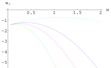
Figure 1: Plot of $\omega_{\Lambda}$ versus $m$ for non-interacting case.

where ($0$) denotes the present time value of the parameters.

Finally, we obtain $\omega_{\Lambda}$ by inserting the above equations in (19). In the evolution of $\omega_{\Lambda}$, the MHDE parameter $m$ plays a crucial role and hence we plot $\omega_{\Lambda}$ against $m$ as shown in Figure (1). Here we consider the present values of fractional energy densities $\Omega^{0}_{\Lambda}=0.73$, $\Omega^{0}_{k}=0.01$, $H_{0}=1$ [40] and $0\leq\Delta_{G}\leq 0.07$ [16]. Plots in turquoise, blue, pink and green curves correspond to values of redshift parameter $z=0.1,0.31,0.5,0.9,$ respectively. We observe that for $z=0.1$, the EoS parameter attains different phases of the universe such as phantom ($0.04<~{}m<0.45$), vacuum DE ($m=0.45,1.56$), quintessence ($0.45<~{}m<1.56$) and then phantom for $m>1.56$. However, for $z=0.1,0.31,0.5,0.9$, the EoS achieves its maximum value $-0.6,-1.2,-1.25,-1.3$, respectively, and remains in the phantom region except $z=0.1$.

2.2 Interacting Case

Here we evaluate EoS parameter in the interacting phenomenon of MHDE with DM by using the same procedure as above. In this case, the equation of continuity may be converted into two non-conserving equations for DM and MHDE, respectively, i.e.,

$$\dot{\rho}_{m}+4H\rho_{m} = \Upsilon,$$ (24)

$$\dot{\rho}_{\Lambda}+4H(\rho_{\Lambda}+p_{\Lambda}) = -\Upsilon,$$ (25)

where $\Upsilon$ denotes the interaction term which can be taken as [27]

$$\Upsilon=4d^{2}H\rho_{\Lambda}.$$

The parameter $d$ is a coupling constant and the selection of its square leads to the condition of decay from DE to DM. We can find $\omega_{0}$ and $\omega_{1}$ by using the above procedure as follows:

$$\omega_{0} = -\frac{3}{2}-d^{2}+\frac{m\pi}{2H_{0}^{2}\sqrt{2\Omega^{0}_{\Lambda}}}\sqrt{1-\frac{2H_{0}^{4}\Omega^{0}_{\Lambda}|\Omega^{0}_{k}|}{m^{2}\pi^{2}}}+\frac{1}{4}\Delta_{G},$$ (26)

$$\omega_{1} = \frac{1}{4}\left[\Omega^{0}_{\Lambda}|\Omega^{0}_{k}|-(1+\Omega^{0}_{\Lambda})\left(\frac{m^{2}\pi^{2}}{H_{0}^{4}\Omega^{0}_{\Lambda}}\right)+\frac{m\pi}{H_{0}^{2}\sqrt{2\Omega^{0}_{\Lambda}}}(-4-\Omega^{0}_{k}+3\right.$$ (27)

$$+ \left.3\Omega^{0}_{\Lambda})+\frac{1}{2}\Delta_{G}(1+\Omega^{0}_{k}-\Omega^{0}_{\Lambda}+2d^{2}\Omega^{0}_{\Lambda})\sqrt{1-\frac{2H_{0}^{4}\Omega^{0}_{\Lambda}|\Omega^{0}_{k}|}{m^{2}\pi^{2}}}\right].$$

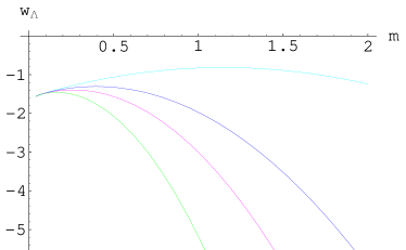
Figure 2: Plot of $\omega_{\Lambda}$ versus $m$ for interacting case.

Inserting these values in Eq.(19), we obtain EoS parameter. In this case, $\omega_{\Lambda}$ evolves two constant parameters $m$ and $d$ (interacting parameter). Figure (2) shows the plot of $\omega_{\Lambda}$ against $m$ by setting $d^{2}=0.1$ and the remaining parameters are the same as in the non-interacting case. Notice that the maximum values of EoS parameter corresponding to the redshift parameter becomes smaller than that of the non-interacting case.

3 Generalized Second Law of Thermodynamics

Now we investigate the validity of GSLT for non-interacting and interacting MHDE with varying G in the non-flat KK universe. According to this law, the sum of entropy of matter inside and at the event horizon remains always positive with the passage of time [41]. Thermodynamics of black hole plays the role of pillar for thermodynamical interpretation of the universe. Bekenstein [42] suggested that, in view of the proportionality relation between entropy of black hole horizon and horizon area, the sum of black hole entropy and the background entropy must be an increasing quantity with time. The first law of thermodynamics gives

$$TdS=pdV+dE,$$ (28)

where $T,~{}S,~{}E$ and $p$ represent temperature, entropy, internal energy and pressure of the system, respectively. Splitting this law for DE, DM and differentiating with respect to time, we obtain

$$\dot{S_{\Lambda}}=\frac{p_{\Lambda}\dot{V}+\dot{E_{\Lambda}}}{T},\quad\dot{S_{m}}=\frac{p_{m}\dot{V}+\dot{E_{m}}}{T}.$$ (29)

The volume, temperature and entropy of horizon in KK universe become [43]

$$V=\frac{\pi^{2}L^{4}}{2},\quad T=\frac{1}{2\pi L},\quad S_{H}=\frac{\pi^{2}L^{3}}{2G}.$$ (30)

Also, we require the following thermodynamical quantities:

$$E_{\Lambda}=\frac{\pi^{2}L^{4}\rho_{\Lambda}}{2},\quad E_{m}=\frac{\pi^{2}L^{4}\rho_{m}}{2}.$$ (31)

Equation (6) can be re-written as

$$\frac{\rho_{m}}{\rho_{\Lambda}}=-1+\frac{1}{\Omega_{\Lambda}}+\frac{\Omega_{k}}{\Omega_{\Lambda}}.$$ (32)

In view of the above equations, we have

$$\dot{S}_{total} = \frac{3m^{2}\pi^{4}L^{6}}{2G}\left[\left(-\omega_{\Lambda}-\frac{1}{\Omega_{\Lambda}}-\frac{\Omega_{k}}{\Omega_{\Lambda}}-\frac{m^{2}\pi^{2}}{4H^{4}\Omega^{2}_{\Lambda}}\right)\sqrt{1-\frac{2H^{4}\Omega_{\Lambda}|\Omega_{k}|}{m^{2}\pi^{2}}}\right.$$ (33)

$$+ \left.\frac{m\pi}{3(2\Omega_{\Lambda})^{\frac{3}{2}}H^{2}}(3-\Delta_{G})\right],$$

where $S_{total}$ is the sum of three entropies. When we substitute the present values of $\Omega_{\Lambda},~{}\Omega_{k}$, $\Delta_{G},~{}\omega_{\Lambda}$ (with $z\leq 0.75$) and $m\geq 0.1$ in the above expression, it remains non-negative for both interacting and non-interacting cases of MHDE i.e., $\dot{S}_{total}\geq 0$.

4 The Statefinder Diagnostic

Here we explore the behavior of statefinder parameters in the above mentioned scenario. These parameters have geometrical diagnostic due to their total dependence on expansion factor. These are defined for a non-flat KK universe as [44]

$$r=\frac{\dddot{a}}{aH^{3}},\quad s=\frac{r-\Omega_{tot}}{3(q-\frac{\Omega_{tot}}{2})},$$ (34)

where $\Omega_{tot}=\Omega_{\Lambda}+\Omega_{m}=1+\Omega_{k}$ and $q$ is the deceleration parameter defined as

$$q=-\frac{\ddot{a}}{aH^{2}}.$$ (35)

The statefinder parameters are dimensionless and exhibit expansion of the universe through higher derivatives of the scale factor. These are a natural companion to the deceleration and Hubble parameters. The pair $(r,s)$ defines the well-known $\Lambda$CDM model at the fixed point $(r,s)=(\Omega_{tot},0)$. Moreover, $r$ can be expressed in terms of the Hubble parameter as

$$r=\frac{\ddot{H}}{H^{3}}-3q-2.$$ (36)

With the help of Eqs.(35) and (36), one can write

$$r=2q^{2}+q-\frac{\dot{q}}{H}.$$ (37)

In the non-interacting case, the time derivative of the deceleration parameter becomes

$$\dot{q}=H[q(-2+\Delta_{G}+2q)-4\Omega_{\Lambda}(1+2\omega_{\Lambda})+2\Omega_{\Lambda}\omega^{\prime}_{\Lambda}].$$

Inserting this in Eq.(37), we obtain

$$r = (3-\Delta_{G})[(1+\Omega_{k})(1-\frac{1}{2}\Delta_{G})+2\omega_{\Lambda}\Omega_{\Lambda}]+4\omega_{\Lambda}\Omega_{\Lambda}$$ (38)

$$\times (1+2\omega_{\Lambda}-\frac{1}{2}\Delta_{G})-2\Omega_{\Lambda}\omega^{\prime}_{\Lambda},$$

$$s = \frac{(3-\Delta_{G})[(1+\Omega_{k})(1-\frac{1}{2}\Delta_{G})+2\omega_{\Lambda}\Omega_{\Lambda}]+4\omega_{\Lambda}\Omega_{\Lambda}}{3[(1+\Omega_{k})(1-\frac{1}{2}\Delta_{G})+2\omega_{\Lambda}\Omega_{\Lambda}-\frac{\Omega_{tot}}{2}]}$$ (39)

$$+ \frac{4\omega_{\Lambda}\Omega_{\Lambda}(2\omega_{\Lambda}-\frac{1}{2}\Delta_{G})-2\Omega_{\Lambda}\omega^{\prime}_{\Lambda}-\Omega_{tot}}{3[(1+\Omega_{k})(1-\frac{1}{2}\Delta_{G})+2\omega_{\Lambda}\Omega_{\Lambda}-\frac{\Omega_{tot}}{2}]},$$

For the interacting case, we differentiate Eq.(5), using (13) and (2.1), and it follows that

$$\frac{\ddot{H}}{H^{3}} = 8+5\Omega_{k}+8\omega_{\Lambda}\Omega_{\Lambda}-2\Delta_{G}(1+\Omega_{k}+\Omega_{\Lambda}\omega_{\Lambda})$$

$$+ 8\Omega_{\Lambda}\omega_{\Lambda}(1+\omega_{\Lambda})-2\Omega_{\Lambda}\omega^{\prime}_{\Lambda}+8d^{2}\Omega_{\Lambda}.$$

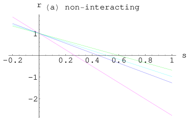
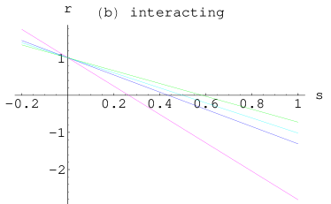
Figure 3: Plots of $r$ versus $s$ for (a) non-interacting and (b) interacting cases.

Consequently, the corresponding statefinder takes the form

$$r = (3-\Delta_{G})[(1+\Omega_{k})(1-\frac{1}{2}\Delta_{G})+2\omega_{\Lambda}\Omega_{\Lambda}]+4\omega_{\Lambda}\Omega_{\Lambda}$$ (40)

$$\times (1+2\omega_{\Lambda}-\frac{1}{2}\Delta_{G})-2\Omega_{\Lambda}\omega^{\prime}_{\Lambda}+8d^{2}\Omega_{\Lambda},$$

$$s = \frac{(3-\Delta_{G})[(1+\Omega_{k})(1-\frac{1}{2}\Delta_{G})+2\omega_{\Lambda}\Omega_{\Lambda}]+4\omega_{\Lambda}\Omega_{\Lambda}}{3[(1+\Omega_{k})(1-\frac{1}{2}\Delta_{G})+2\omega_{\Lambda}\Omega_{\Lambda}-\frac{\Omega_{tot}}{2}]}$$ (41)

$$+ \frac{(2\omega_{\Lambda}-\frac{1}{2}\Delta_{G})-2\Omega_{\Lambda}\omega^{\prime}_{\Lambda}+8d^{2}\Omega_{\Lambda}-\Omega_{tot}}{3[(1+\Omega_{k})(1-\frac{1}{2}\Delta_{G})+2\omega_{\Lambda}\Omega_{\Lambda}-\frac{\Omega_{tot}}{2}]}.$$

We can easily find a single relation of $r$ in terms of $s$ and draw $s-r$ plane as shown in Figure (3) for ($a$) non-interacting and ($b$) interacting MHDE. Plots in pink, blue, turquoise and green colors are drawn at different physically acceptable values of $m=0.21,0.61,0.73,0.91$ (as already discussed in [38]), respectively, for non-interacting as well as interacting cases. Also, we fix $z=0.1,d^{2}=0.1$ and recover the $\Lambda$CDM model in both cases.

5 Concluding Remarks

We have investigated the behavior of EoS parameter, GSLT and statefinder for the MHDE (non-interacting and interacting with DM) with variable $G$ correction in non-flat KK universe enclosed by future event horizon. Actually, the MHDE exhibits the dynamical nature of the vacuum DE through its parameter $m$. We have evaluated the EoS parameter with respect to $m$ for different ranges of $z=0.1,0.31,0.5,0.9$. It is found that the interacting and non-interacting MHDE behave like a quintom model for a comparatively smaller value of the redshift parameter, i.e., $z=0.1$ with the assumptions of the present values of the other parameters. For other values of $z$, it evolutes the universe in phantom DE era in view of increasing $m$. Our results about evolution of MHDE with varying $G$ shows compatibility with the present observations for flat, non-flat FRW [16, 26] and flat KK universes [38] enclosed by future event horizon that it can cross the phantom divide.

Secondly, we have explored that GSLT is satisfied with $z\geq 0.75$ for the universe describing phantom evolution. Moreover, we have obtained the evolution of non-interacting and interacting MHDE in the statefinder plane for different best fitted values of $m,~{}d$ (for interacting case) and $z=0.1$. The trajectories of $s$-$r$ plane have been achieved with respect to different model parameters which is started from right to left. Notice that the parameters $s$ and $r$ show decreasing and increasing behavior, respectively, with the phantom evolution of the KK universe.

References

• [1] Riess, A.G. et al.: Astron. J. 116(1998)1009; Perlmutter, S. et al.: Astrophys. J. 517(1999)565.
• [2] Peebles, P.J.E.: Rev. Mod. Phys. 75(2003)559.
• [3] Ratra, B and Peebles, P.J.E.: Phys. Rev. D37(1988)3406.
• [4] Armendariz-Picon, C., Damour, T and Mukhanov, V.: Phys. Lett. B458(1999)209; Chiba, T., Okabe, T. and Yamaguchi, M.: Phys. Rev. D62(2000)023511.
• [5] Caldwell, R.R.: Phys. Lett. B545(2002)23; Carroll, S.M., Hoffman, M. and Trodden, M.: Phys. Rev. D68(2003)023509.
• [6] Feng, B., Wang X.L. and Zhang, X.M.: Phys. Lett. B607(2005)35.
• [7] Padmanabhan, T.: Phys. Rev. D66(2002)021301; Bagla, J.S., Jassal, H.K. and Padmanabhan, T.: Phys. Rev. D67(2003)063504.
• [8] Kamenshchik, A.Y., Moschella, U. and Pasquier, V.: Phys. Lett. B511(2001)265; Bento, M.C., Bertolami, O. and Sen, A.A.: Phys. Rev. D 66(2002)043507; Zhang, X., Wu, F.Q. and Zhang, J.: JCAP 01(2006)003.
• [9] Hsu, S.D.H.: Phys. Lett. B594(2004)13.
• [10] Li, M.: Phys. Lett. B603(2004)1.
• [11] Cai, R.G.: Phys. Lett. B657(2007)228.
• [12] Ng, Y.J.: Phys. Rev. Lett. 86(2001)2946; Arzano, M., Kephart, T.W. and Ng, Y.J.: Phys. Lett. B649(2007)243.
• [13] Zhang, X. and Wu, F.Q.: Phys. Rev. D72(2005)043524.
• [14] Susskind, L.: J. Math. Phys. 36(1995)6377.
• [15] Cohen, A., Kaplan, D. and Nelson, A.: Phys. Rev. Lett. 82(1999)4971.
• [16] Jamil, M., Saridakis, E.N., and Setare, M.R.: Phys. Lett. B679(2009)172.
• [17] Nojiri, S. and Odintsov, S.D.: Int. J. Geom. Meth. Mod. Phys. 4(2007)115.
• [18] Linder, E.V.: Phys . Rev. D81(2010)127301.
• [19] Brans, C.H. and Dicke, R.H.: Phys. Rev. 124(1961)925.
• [20] Dutta, S and Saridakis, E.N.: JCAP 01(2010)013.
• [21] Kaluza, T.: Zum Unitatsproblem der Physik Sitz. Press. Akad. Wiss. Phys. Math. k1 (1921)966; Klein, O.: Zeits. Phys. 37(1926)895.
• [22] Wesson, P.S.: Gen. Relativ. Gravit. 16(1984)193; Spacetime-Matter Theory (World Scientific, 1999); Bellini, M.: Nucl. Phys. B660(2003)389.
• [23] Myers, R.C.: Phys. Rev. D35(1987)455.
• [24] Gong, Y. and Li, T.: Phys. Lett. B683(2010)241.
• [25] Huang, Q.G. and Li, M.: JCAP 04(2004)013.
• [26] Lu, J. et al.: JCAP 03(2010)031.
• [27] Sheykhi, A.: Phys. Rev. D84(2011)107302; Karami, K., Ghaffari, S. and Soltanzadeh, M.M.: Class. Quantum Grav. 27(2010)205021.
• [28] Setare, M.R.: JCAP 01(2007)023; Sheykhi, A.: Class. Quantum Grav. 27(2010)025007.
• [29] Mazumder, M. and Chakraborty, S.: Gen. Relativ. Gravit. 42(2010)813.
• [30] Sahni, V. et al.: JETP Lett. 77(2003)201.
• [31] Alam, U. et al.: Mon. Not. R. Astron. Soc. 344(2003)1057.
• [32] Feng, C.: Phys. Lett. B670(2008)231.
• [33] Setare, M.R., Zhang, J. and Zhang, X.: JCAP 03(2007)007; Setare, M.R. and Jamil, M.: Gen. Relativ. Gravit. 43(2011)293.
• [34] Malekjani, M., Khodam-Mohammadi, A. and Nazari-pooya, N: Astrophys. Space Sci. 332(2011)515.
• [35] Chakraborty, S. et al.: Int. J. Theor. Phys. (2012, to appear), arXiv:1111.3853.
• [36] Liu, D.J., Wang, H. and Yang, B.: Phys. Lett. B694(2010)6.
• [37] Sharif, M. and Khanum, F.: Gen. Relativ. Gravit. 43(2011)2885.
• [38] Sharif, M. and Jawad, A.: Astrophys. Space Sci. 337(2012)789.
• [39] Ozel, C., Kayhan, H. and Khadekar, G.S.: Ad. Studies. Theor. Phys. 4(2010)117.
• [40] Paul, B.C., Debnath, P. S. and Ghose, S.: Phys. Rev. D79(2009)083534.
• [41] Izquierdo, G. and Pav$\acute{o}$n, D.: Phys. Lett. B633(2006)420.
• [42] Bekenstein, J.D.: Phys. Rev. D7(1973)2333.
• [43] Cai, R.G. and Kim, S.P.: JHEP 0502(2005)050.
• [44] Evans, A.K.D. et al.: Astron. Astrophys. 430(2005)399.