Magnetic-field-induced dimensional crossover in the organic metal $\alpha$-(BEDT-TTF)₂KHg(SCN)₄

Abstract

The field dependence of interlayer magnetoresistance of the pressurized (to the normal state) layered organic metal $\alpha$-(BEDT-TTF)₂KHg(SCN)₄ is investigated. The high quasi-two-dimensional anisotropy, when the interlayer hopping time is longer than the electron mean-free time and than the cyclotron period, leads to a dimensional crossover and to strong violations of the conventional three-dimensional theory of magnetoresistance. The monotonic field dependence is found to change from the conventional behavior at low magnetic fields to an anomalous one at high fields. The shape of Landau levels, determined from the damping of magnetic quantum oscillations, changes from Lorentzian to Gaussian. This indicates the change of electron dynamics in the disorder potential from the usual coherent three-dimensional regime to a new regime, which can be referred to as weakly coherent.

I Introduction

Highly anisotropic layered conductors in a strong magnetic field may undergo a dimensional crossover from three-dimensional (3D) to almost two-dimensional (2D) electron dynamics when the interlayer transfer integral $t_{\perp}$ becomes smaller than the other relevant parameters: the scattering rate and the cyclotron frequency. This crossover may change the electronic transport properties in various layered compounds: organic metals, heterostructures, intercalated compounds, superconductive cuprates and pnictides, cobaltates etc. Scattering by crystal disorder is one of the most frequently discussed mechanisms of breaking the interlayer band transport in layered metals. If the scattering rate $\tau^{-1}$ is larger than the interlayer hopping rate, $\tau_{h}^{-1}\sim t_{\perp}/\hbar$, the quasiparticle momentum and Fermi surface are only defined within conducting layers, i.e. become strictly 2D. However, the interlayer electron tunneling may still be ”coherent” and conserve the in-plane electron momentum. The corresponding regime was called ”weakly incoherent”.kenz98 ; MosesMcKenzie1999 In the literature there has been a long-time discussion, supported by theoreticalMosesMcKenzie1999 ; Abrikosov1999 ; Lundin2003 ; OsadaIncoherent ; Ho ; Gvozd2007 ; McKenzie2007 ; Maslov ; WIPRB2011 ; WIJETP2011 ; WIFNT2011 ; Incoh2009 and experimentalIncoh2009 ; Zuo1999 ; Wosnitza2002 ; CrossoverNAture2002 ; MarkPRL2006 ; Ardavan2006 ; zver96 arguments, whether this ”weakly incoherent” regime can be distinguished from the usual three-dimensional (3D) electron transport. Up to now, no considerable qualitative differences between 3D and ”weakly incoherent” regimes have been suggested or observed. The only significant predicted change in the ”weakly incoherent” regime is the absence of the narrow ”coherence peak” on the angular dependence of magnetoresistance when the magnetic field is directed along the conducting layerskenz98 ; MosesMcKenzie1999 . However, the absence of even this subtle feature in the ”weakly incoherent” regime has not received a sound proof yet. Hence, for a long time it was believedkenz98 ; MosesMcKenzie1999 ; McKenzie2007 ; Maslov ; kuma92 that in this regime the interlayer resistivity $\rho_{\perp}(T)$ is nearly identical to that in the fully coherent three-dimensional (3D) case.

Another possible mechanism of dimensional crossover is associated with external magnetic field $B$.CommentT Indeed, the behavior of magnetic quantum oscillations (MQO) is substantially modifiedShoenberg ; PhSh ; Shub ; SO ; ChampelMineev ; Gvozd2007 ; harr96 ; mk04 when the cyclotron frequency $\omega_{c}=eB/m_{c}$ becomes larger than the interlayer hopping rate $\tau_{h}^{-1}$. However, the existing theories predict no significant changes in the electron dynamics at weak (but coherent) interlayer electron hopping unless additional mechanisms of interlayer electron transport such as interlayer hopping via the resonance impuritiesAbrikosov1999 ; Maslov ; Incoh2009 or boson-assistedLundin2003 ; Ho tunneling are concerned.commentFISDW

In this work we show, that the parameter $b_{\ast}\equiv\hbar\omega_{c}/t_{\perp}$ drives a transition between two qualitatively different regimes of electron dynamics. There are several principal distinctions in the field dependence of interlayer magnetoresistance at $b_{\ast}\gg 1$, originating from the qualitatively different influence of disorder on electronic properties. These changes cannot be explained by a simple extension of the formulas in Refs. Shub ; ChampelMineev to the case $b_{\ast}\gg 1$, which unambiguously separates this regime from $b_{\ast}\ll 1$. We refer to this new regime as ”weakly coherent”: it implies a conservation of the in-plane electron momentum by the interlayer tunneling term in the Hamiltonian; on the other hand, the time scale of this tunneling is much larger than the cyclotron period. Note that the parameter $b_{\ast}\equiv\hbar\omega_{c}/t_{\perp}$ is completely different from the parameter $\hbar/t_{\perp}\tau$, which was usedkenz98 ; MosesMcKenzie1999 to separate the coherent and weakly incoherent regimes. The proposed weakly coherent regime imposes no limitation on the value of parameter $\hbar/t_{\perp}\tau$. Therefore, strictly speaking, there is no direct relation between the weakly incoherent and the newly defined weakly coherent regimes. On the other hand, the compounds satisfying the condition of the weakly incoherent regime are automatically driven to the weakly coherent regime by a strong magnetic field such that $\omega_{c}\tau>1$.

Here we present a joint theoretical and experimental study of the weakly coherent regime, on the example of the layered organic metal $\alpha$-(BEDT-TTF)₂KHg(SCN)₄. The title compound has a strong anisotropy with the interlayer transfer integral $t_{\perp}\sim 30$ $\mu$eV.MarkPRL2006 At ambient pressure it undergoes a charge-density-wave transition at $\approx 8.5$ K, which can be suppressed by applying an external pressure $P>P_{c}\approx 2.5$ kbar.andres01 ; andres05 . To avoid complications related to the zero-field and magnetic-field-induced charge-density-wave states andres12 , a pressure of 6 kbar, considerably exceeding $P_{c}$ and temperatures above 1 K were used, so that the compound was in the fully normal metallic state in our experiment. The corresponding Fermi surface consists of a cylinder (quasi-2D band) and a pair of weakly warped open sheets (quasi-1D band). As will be shown below, the interlayer conductivity in fields above 2 T, is largely determined by the quasi-2D carriers, so we will restrict our analysis to the case of a cylindrical Fermi surface. The weakly-coherent criterion $b_{\ast}\gg 1$ in this compound is satisfied at an easily accessible field $B_{z}\gg t_{\perp}m_{c}/e\hbar\simeq 0.3$ T, where $m_{c}\approx 1.3m_{\mathrm{e}}$ is the relevant cyclotron mass.

II Theoretical background

The first step in the theoretical analysis of the weakly coherent regime was made recently in Refs. WIPRB2011 ; WIJETP2011 ; WIFNT2011 , where it was shown that in the regime where weakly coherent and weakly incoherent criteria overlap, the earlier theoretical conclusionkenz98 ; MosesMcKenzie1999 ; McKenzie2007 that the interlayer resistivity $\rho_{\perp}(T)$ is identical to that in the fully coherent three-dimensional (3D) case is not valid. The new analysis, going beyond the constant relaxation time approximation used in the earlier works,kenz98 ; MosesMcKenzie1999 ; ChampelMineev ; harr96 has predicted several qualitatively new features of interlayer magnetoresistance in the weakly coherent regime.

The first prediction is a monotonic growth of the magnetoresistance, averaged over MQO, with an increase of magnetic field, parallel to the current and perpendicular to the conducting layers.WIPRB2011 ; WIJETP2011 ; WIFNT2011 This increase, contradicting the classical theory of MR even for quasi-2D metals,Shub ; ChampelMineev is due to the enhancement of the effect of short-range impurities caused by a magnetic field and follows directly from the monotonic growth $\propto\sqrt{B_{z}}$ of the Landau level (LL) broadening due to the short-range impurity scattering.Ando It is not related to the low crystal symmetry. The field dependence of the nonoscillating component of the interlayer conductivity is given by WIPRB2011 ; WIJETP2011 ; WIFNT2011

$$\bar{\sigma}_{zz}\left(B\right)\approx\sigma_{0}\left[\left(\alpha\omega_{c}\tau\right)^{2}+1\right]^{-1/4}.$$ (1)

The numerical coefficient $\alpha\approx 2$ before $\omega_{c}\tau$ is not universal and slightly depends on the shape of LLs.WIJETP2011

The second prediction for the weakly coherent regimeWIPRB2011 is a modification of the angular dependence of magnetoresistance due to a decrease of the effective mean scattering time $\tau$ with an increase of the interlayer component $B_{z}=B\cos\theta$ of magnetic field [see Eqs. (36) and (37) of Ref. WIPRB2011 ]. An accurate comparison of this effect with experiment on $\alpha$-(BEDT-TTF)₂KHg(SCN)₄ requires elimination of the angular dependence associated with the quasi-1D parts of the Fermi surface which is beyond the scope of this work.

The third prediction of the theory in Refs. WIPRB2011 ; WIJETP2011 ; WIFNT2011 , is the growth of the Dingle temperature of MQO with an increase of magnetic field, and, hence, the stronger damping of MQO. Naively, since the LL width $\Gamma\equiv\hbar/2\tau_{B}$ in the single-site approximationAndo grows at $\omega_{c}\tau\gg 1$ as $\tau/\tau_{B}\approx\left[\left(2\omega_{c}\tau\right)^{2}+1\right]^{1/4}$ $\propto\sqrt{B_{z}}$, one would expect the similar square-root growth of the Dingle temperature $T_{D}\left(B_{z}\right)$. However, this simple conclusion is incorrect for two reasons: (i) the square-root growth of the LL width appears only for a short-range impurity potential, while in organic and many other layered metals the main contribution to the LL broadening often comes from a long-range disorder potentialSO ; (ii) the MQO damping factor is determined not only by the width of LLs, but also by their shape.

To check this we substitute the density of state (DoS)

$$\rho\left(\varepsilon\right)=\sum_{n\geq 0}D\left[\varepsilon-\hbar\omega_{c}\left(n+1/2\right)\right]$$ (2)

to the expression for the interlayer conductivity, obtained as a linear response from the Kubo formula [see Eq. (14) of Ref. WIJETP2011 and note that $\rho\left(\varepsilon\right)=-$Im$G_{R}(\varepsilon)/\pi$]

$$\sigma_{zz}=\pi\sigma_{0}\Gamma_{0}\hbar\omega_{c}\sum_{s=\uparrow,\downarrow}\int d\varepsilon\left[-n_{F}^{\prime}(\varepsilon)\right]\left|\rho_{s}\left(\varepsilon\right)\right|^{2}.$$ (3)

As long as the shape and width of LLs do not change with temperature, the temperature harmonic damping factor $R_{T}$ is described by the usual Lifshitz-Kosevich expression: $R_{T}\left(k\right)=kX/\sinh\left(kX\right)\,$, where $X\equiv 2\pi^{2}k_{B}T/\hbar\omega_{c}$. Now substituting Eq. (2) to Eq. (3) and applying the Poisson summation formula, we obtain at $N_{\mathrm{LL}}\gg 1$

$$\frac{\sigma_{zz}}{\bar{\sigma}_{zz}}=\sum_{k=-\infty}^{\infty}\left(-1\right)^{k}\exp\left(\frac{2\pi ik\mu}{\hbar\omega_{c}}\right)R_{\mathrm{D}}\left(k\right)R_{T}\left(k\right)R_{\mathrm{S}}\left(k\right),$$ (4)

where the averaged over MQO interlayer conductivity $\bar{\sigma}_{zz}$ is given by Eq. (1), the spin-splitting damping factorShoenberg $R_{\mathrm{S}}\left(k\right)=\cos\left(\pi kgm^{\ast}/2\right)$, $\mu$ is the Fermi energy, $m^{\ast}\equiv m_{c}/m_{\mathrm{e}}$ is the effective cyclotron mass normalized to the free electron mass, and the Dingle factor

$$R_{\mathrm{D}}\left(k\right)=2\pi\Gamma\int_{-\infty}^{\infty}\exp\left(\frac{2\pi ikE}{\hbar\omega_{c}}\right)\left|D\left(E\right)\right|^{2}dE.$$ (5)

The traditional Lorentzian shape of LLs with the halfwidth $\Gamma$, $D_{\mathrm{L}}\left(E\right)=\left(\pi\Gamma\right)^{-1}/\left[1+\left(E/\Gamma\right)^{2}\right]$, after substitution to Eq. (4) gives the Dingle factor

$$R_{\mathrm{DL}}\left(k\right)=\exp\left(-2\pi k\Gamma/\hbar\omega_{c}\right)\left(1+2\pi k\Gamma/\hbar\omega_{c}\right).$$ (6)

As was shown in Refs. ShubCondMat ; ChampelMineev ; Shub , it differs from the standard Dingle factor, valid in the case $t_{\perp}\gg\hbar\omega_{c}$,

$$R_{\mathrm{DL}}\left(k\right)\approx\exp\left(-2\pi k\Gamma/\hbar\omega_{c}\right).$$ (7)

However, this difference does not considerably change the Dingle plot, i.e. the field dependence of the logarithm of the Dingle factor:

$$\ln R_{\mathrm{DL}} = -2\pi\Gamma/\hbar\omega_{c}+\ln\left(1+2\pi k\Gamma/\hbar\omega_{c}\right)$$ (8)

$$= -B_{0}/B+\ln\left(1+B_{0}/B\right),$$

where $B_{0}=2\pi k\Gamma m_{c}/\hbar e$. In a strong field, when $\omega_{c}\tau\gg 1$ the ratio $B_{0}/B$ is small and the correction $\ln\left(1+B_{0}/B\right)\ll 1$. In the opposite limit, $\omega_{c}\tau\ll 1$ or $B\ll B_{0}$, the field dependence coming from the first term in Eq. (8) is much stronger than weak logarithmic dependence from the second term. Hence, the factor $(1+2\pi k\Gamma/\hbar\omega_{c})$ gives only a small correction to the field dependence of the MQO amplitude [see Fig. 3 below for comparison of Eqs. (6) and (7), and one usually can apply Eq. (7) for the analysis of the Dingle plots.

If one assumes $\Gamma$ to be independent of $B$, Eq. (7) gives the standard result:

$$R_{\mathrm{DL}}\left(k\right)\approx\exp\left(-\mathrm{const}\cdot k/B_{z}\right),$$ (9)

while if $\Gamma\propto\sqrt{B_{z}}$ as in the self-consistent Born approximation,Ando Eq. (7) gives

$$R_{\mathrm{DL}}^{\ast}\left(k\right)\approx\exp\left(-\mathrm{const}\cdot k/\sqrt{B_{z}}\right).$$ (10)

The Gaussian shape of LLs, $D_{\mathrm{G}}\left(E\right)=\left(\sqrt{\pi}\Gamma\right)^{-1}\exp\left(-E^{2}/\Gamma^{2}\right)$, gives the Dingle factor

$$R_{\mathrm{DG}}\left(k\right)=\sqrt{\pi/2}\exp\left[-\left(\pi k\Gamma/\hbar\omega_{c}\right)^{2}/2\right].$$ (11)

The theory predicts the Gaussian shape of the Landau levels (for a review see, e.g., Ref. KukushikUFN1988 ) for a physically reasonable white-noise or Gaussian correlator of the disorder potential $U\left(\mathbf{r}\right)$:

$$Q\left(\mathbf{r}\right)=\left\langle U\left(\mathbf{0}\right)U\left(\mathbf{r}\right)\right\rangle\propto\exp\left(-r^{2}/2d^{2}\right).$$ (12)

For a long-range disorder potential, when $d\gg l_{B}\equiv\sqrt{\hbar/eB}$, the LL width $\Gamma$ is independent of $B$ (see, e.g., Eq. (2.9) of Ref. KukushikUFN1988 ). Then even the magnetic-field dependence of the Dingle factor is different from the 3D case:

$$R_{\mathrm{DG}}\left(k\right)=\sqrt{\pi/2}\exp\left[-\mathrm{const}\cdot k^{2}/B_{z}^{2}\right].$$ (13)

For a short-range impurity potential $d\ll l_{B}$, one obtains the white-noise correlator $Q\left(\mathbf{r}\right)\approx\mathrm{const}\cdot\delta\left(\mathbf{r}\right)$. Then the dependence of the level width on magnetic field, in a strong field, at $N_{LL}\gg 1$, $\Gamma\propto\sqrt{B_{z}}$ is in agreement with Refs. Ando ; Brezin . The Dingle factor (11) in this case has a similar to the 3D case magnetic-field dependence, but a stronger damping of higher harmonics:

$$R_{\mathrm{DG}}^{\ast}\left(k\right)=\sqrt{\pi/2}\exp\left[-\mathrm{const}\cdot k^{2}/B_{z}\right].$$ (14)

Eqs. (9),(10),(13) and (14) suggest that it is possible not only to distinguish experimentally between the Lorentzian and Gaussian shapes of LLs but also to obtain information about the range of scatterers and the physical origin of the LL broadening. For the Gaussian shape of LLs the higher harmonics of MQO are much stronger damped than for Lorentzian LL shape because the exponent contains $k^{2}$ instead of $k$. The Dingle plot, i.e. the plot of the logarithm of the MQO amplitudes as a function of inverse magnetic field, gives additional information about the origin of the LL broadening.

III Experimental results and discussion

III.1 Nonoscillating magnetoresistance

Plotted in Fig. 1 are the raw data on the field dependence of interlayer magnetoresistance $R_{zz}\left(B\right)$ of $\alpha$-(BEDT-TTF)₂KHg(SCN)₄, (dashed grey curve) in a field perpendicular to layers, $\mathbf{B}\|z$, along with its monotonic background part $R_{zz}^{\mathrm{B}}$ (solid black curve), obtained by filtering out the MQO component. Note that due to the very high amplitude of the oscillations comparable to the monotonic background, the data should be treated in terms of conductivity $\sigma_{zz}(B)\propto 1/R_{zz}(B)$ rather than resistivity. Hence, for extracting the background, the as-measured resistance was first inverted, then the oscillations were subtracted using a Fourier filter and the result was again inverted to obtain $R_{zz}^{\mathrm{B}}(B)$ shown in Fig. 1.

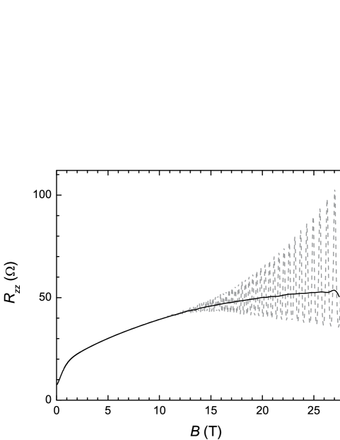
Figure 1: Interlayer magnetoresistance of $\alpha$-(BEDT-TTF)₂KHg(SCN)₄ measured as a function of magnetic field perpendicular to the layers, at $T=1.6$ K (dashed grey line) and its monotonic component $R_{zz}^{\mathrm{B}}(B)$ (solid black line) obtained by filtering out the MQO, see text.

The theoryWIPRB2011 ; WIJETP2011 ; WIFNT2011 predicts that the background magnetoresistance changes proportional to $\sqrt{B}$ in the weakly coherent regime when $\omega_{c}\tau\gg 1$, see Eq. (1) above.

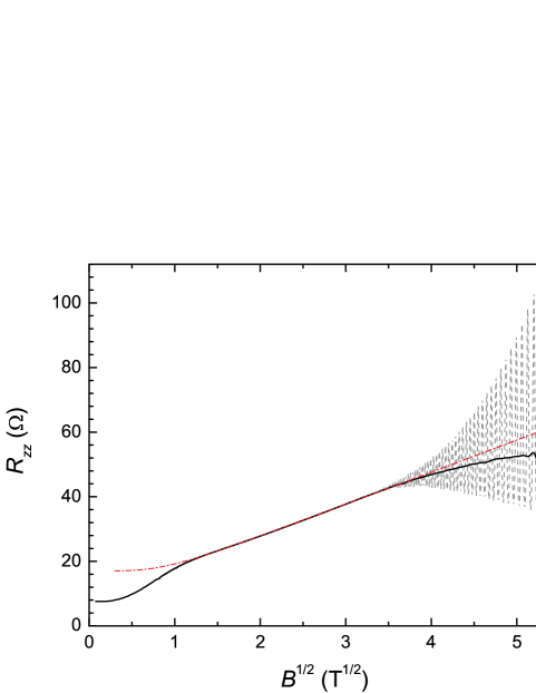
Figure 2: (Color online) The same data as in Fig. 1 plotted versus $\sqrt{B}$ (dashed grey and solid black lines). At fields between 1.5 and 16 T the magnetoresistance is linear in this scale. The fit to Eq. (1) in this field range (dashed-dotted red line) yields the transport scattering time $\tau=4.3$ ps.

To compare this prediction with the observed dependence $R_{zz}\left(B\right)$, in Fig. 2 we plot the data on $R_{zz}$ as function of $\sqrt{B}$. From this plot one can see that background magnetoresistance is indeed perfectly linear in this scale in the range $1.5\mathrm{\;T}<B<16$ T. One can fit the data in this range by modelling the resistance as a sum of a term $\bar{R}_{zz}(B)\propto 1/\bar{\sigma}_{zz}(B)$, determined by Eq. (1), and a field-independent term comparable to $\bar{R}_{zz}(B=0)$. The fit shown as a dashed-dotted line in Fig. 2 yields an estimation for the zero-field scattering time $\tau=4.3$ ps (using $\alpha=2$). The $B$-independent term included in the fit appears due to scattering on dislocations and/or phonons, which does not depend on magnetic field and contributes to the total scattering rate $1/\tau$.

At fields below 1.5 T the strong-field criterion is not fulfilled for this crystal, which leads to a deviation from the linear $\sqrt{B}$-dependence. Additionally, one has to take into account the influence of carriers on the quasi-1D part of the Fermi surface contributing about the same density of states as the quasi-2D carriers considered here. The part of $\sigma_{zz}$ originating from the quasi-1D Fermi surface rapidly (approximately quadratically) decreases with increasing field at all field orientations except the vicinity of commensurate directions, when the field is aligned along one of the crystal lattice translation vectors (so-called Lebed magic angles) mk04 ; osad92 ; lebe03 . Due to the low crystal symmetry of $\alpha$-(BEDT-TTF)₂KHg(SCN)₄, the nearest commensurate direction is considerably, by $\approx 13^{\circ}$, tilted away from the $z$-axis.rous96 Therefore, the contribution of quasi-1D carriers to $\sigma_{zz}$ is strongly suppressed under a magnetic field $B\gtrsim B_{0}=\hbar/(e\tau v_{F}a_{z}\tan 13^{\circ})$ applied perpendicular to layers. Substituting the scattering time $\tau=4.3$ ps , Fermi velocity on the quasi-1D Fermi sheetsmk09 $v_{F}=1.2\times 10^{5}$ m/s, and the interlayer lattice parameterrous96 $a_{z}=2.0$ nm, we estimate $B_{0}\approx 2.7$ T. Therefore, we attribute the steeper slope of the magnetoresistance observed at low fields with the ”freezing-out” of quasi-1D carriers. At fields above $\sim 2$ T the conductivity is believed to be dominated by the carriers on the quasi-2D Fermi surface.

At fields $B>16$ T, when the amplitude of the oscillations becomes of the same order as the background component $R_{zz}^{\mathrm{B}}(B)$, the terms quadratic in the amplitude of MQO give an additional contribution to the monotonic part of conductivity in a way similar to that described by Eqs. (19),(21) of Ref. Shub . This additional contribution can be estimated as $\Delta\sigma_{zz}\propto R_{D\ast}^{2}\approx\exp\left(-2\pi/\omega_{c}\tau\right)$, where the Dingle factor $R_{D\ast}$ is determined by only short-range scattering. Substituting $\tau=4.3$ ps and the effective electron mass $m^{\ast}=1.3$ we obtain $\Delta\sigma_{zz}\propto\exp\left(-B_{\ast}/B\right)$, where $B_{\ast}\approx 11$ T. This explains the small deviation of the background resistivity from the linear dependence at $B>16$ T in Fig. 2. Thus, in the whole, the data in Fig. 2 are considered as a firm evidence of the weakly-coherent interlayer transport regime in this compound.

III.2 Field-induced crossover in magnetic quantum oscillations

Fig. 3 shows the Dingle plot for the first harmonic of MQO. One can see that, contrary to the predictions of the 3D theory of MQO, this plot is not linear in high magnetic field. This excludes the theoretical possibilities, leading to the Dingle factors given by Eqs. (9),(10) and (14). As was argued in Section II, and follows from the comparison between the dashed and solid lines in Fig. 3, the difference between Eqs. (7) and (6) on the Dingle plot is negligible and cannot explain the observed deviation from the linear behavior. On the other hand, the same logarithm of the MQO Dingle factor plotted as function of $1/B^{2}$ gives a very nice linear dependence (see Fig. 4) at field $B>12$ T, which supports the scenario represented by Eq. (13). The LL width $\Gamma$ for $B>12$ T is field-independent, suggesting that the main contribution to the LL broadening comes from the long-range random potential, which changes on the length $d\gg l_{B}$ and gives local variations of the Fermi energy. This long-range potential only damps the MQO but it does not affect the background (averaged over MQO) conductivity because it does not produce a significant electron scattering and relaxation of electron momentum. This situation is similar to that observed in Ref. SO , where the long-range disorder potential only damped the fast MQO but did not damp the slow oscillations of magnetoresistance. Hence, Eq. (1) remains valid, because $\Gamma=\hbar/2\tau$ is determined by short-range impurities and increases in strong magnetic field $\propto\sqrt{B}$. The fact that LL broadening is Gaussian is also very important: it means that electron dynamics in $\alpha$-(BEDT-TTF)₂KHg(SCN)₄ under a strong field is indeed substantially different from that in 3D metals where the impurity scattering leads to a finite electron lifetime and produces the Lorentzian level broadening.

Figure 3: Dingle plot, i.e. the logarithm of the MQO amplitude, divided by the temperature damping factor $R_{T}$, as a function of inverse magnetic field $1/B$. The dashed line is a fit of the data at fields below 12 T to Eq. (7) with field-independent $\Gamma/k_{B}=12.9$ K, and the solid line is the fit to Eq. (6).

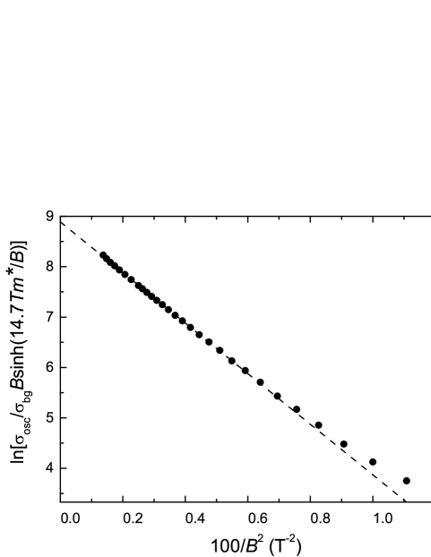
Figure 4: The same data as in Fig. 3 plotted against $1/B^{2}$. For fields $B>12$ T the data is nicely fitted by a straight (dashed) line in agreement with Eq. (13), implying a Gaussian LL broadening with the halfwidth $\Gamma/k_{B}=10.5$ K determined by a long-range scattering potential.

At fields $B<12$ T the dependence in Fig. 4 deviates from linear, suggesting a crossover from the high-field Gaussian LL shape to another shape at lower field, probably, to the Lorentzian shape with a field-independent width $\Gamma$. The linear fit of the Dingle plot in Fig. 3 at $9.5\mathrm{\;T}<B<12$ T gives the LL width $\Gamma/k_{B}=\pi T_{D}\approx 12.9$ K, which is $6$ times greater than one would naively expect from the transport relaxation time $\tau\approx 4.3$ ps determined by short-range scattering. This means that the LL broadening is determined by the long-range disorder potential, which does not produce electron scattering. Fitting of the high-field Dingle factor in Fig. 4 by Eq. (11) gives a comparable LL width $\Gamma/k_{B}\approx 10.5$ K.

Now we use the obtained values of $\Gamma$ to analyze the damping of MQO harmonics and to compare the theoretical predictions for the harmonic amplitudes for both LL shapes with the experimental data. We remind that, taking into account the large amplitude of the oscillations, the analysis is performed for inverse resistance $1/R_{zz}(B)\propto\sigma_{zz}(B)$.

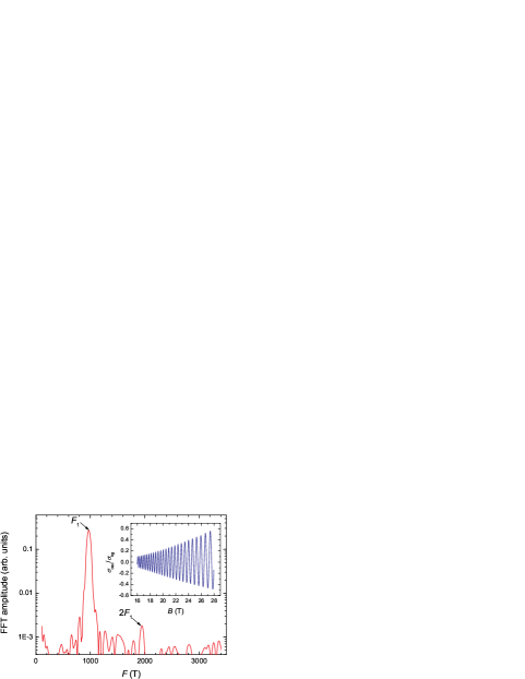
Figure 5: (Color online) FFT spectrum of the oscillations in the interlayer conductivity in the field range $16\mathrm{\;T}<B<28$ T, as shown in the inset.

Fig. 5 shows the fast Fourier transform (FFT) of the oscillatory component of inverse resistance normalized to the field-dependent nonoscillating background. The data is taken in the field window $16\mathrm{\;T}<B<28$ T, as shown in the inset in Fig. 5. One can see that the Fourier spectrum is almost completely dominated by one fundamental harmonic. The amplitude of the second harmonic only slightly exceeds the noise, while the third harmonic is not resolved within the present accuracy. The ratio of the FFT amplitudes of the first and second harmonics averaged over the given field window is $A_{2}/A_{1}\approx 150$, while the first harmonic amplitude normalized to the nonoscillating background increases from $A_{1}\approx 0.1$ at $B=16$ T to $A_{1}\approx 0.5$ at $B=28$ T (see the inset in Fig. 5). For the analysis we take the average (in the $1/B$-scale) value $B_{a}=20.4$ T, where the experimentally obtained normalized amplitudes are $A_{\mathrm{1,exp}}\approx 0.25$ and $A_{\mathrm{2,exp}}\approx 1.7\times 10^{-3}$. The temperature in the experiment is $T\approx 1.6$ K, and the electron effective mass at pressure $6$ kbar is $m^{\ast}\approx 1.3$. This gives $X\equiv 2\pi^{2}k_{B}T/\hbar\omega_{c}\approx 1.50$ at $B_{a}=20.4$ T, and the temperature damping factors of the first and second harmonics are $R_{T}\left(1\right)=0.70$ and $R_{T}\left(2\right)=0.30$. The experimental error bar in determination of the electron effective mass gives the possible errors in the temperature damping factor $\sim 5\%$ and $\sim 15\%$ for the first and second harmonic, respectively. The spin reduction factor $R_{\mathrm{S}}$ can be evaluated from spin-zeros experiments. So far, such experiments have been done for $\alpha$-(BEDT-TTF)₂KHg(SCN)₄ only at ambient pressure, (at high magnetic fields, where the CDW gap is strongly suppressed), yieldinggfactorSasaki ; gfactorHarrison $gm^{\ast}=3.65\pm 0.02$. Making a correction to the pressure-dependent effective mass, which changes from $m^{\ast}\approx 2.0$ at ambient pressure to 1.3 at 6 kbar, and assuming a pressure-independent $g$-factor we substitute $gm^{\ast}=2.37$ in the spin reduction factor to obtain a rough estimate $R_{\mathrm{S}}(1)\simeq 0.8$ and $R_{\mathrm{S}}(2)\simeq 0.4$.

For the Lorentzian LL shape with field-independent $\Gamma/k_{B}=12.9$ K one obtains from Eq. (7) at $B_{a}=20.4$ T the Dingle factors $R_{\mathrm{DL}}\left(1\right)\approx 0.022$ and $R_{\mathrm{DL}}\left(2\right)\approx 0.00047$. The predicted harmonic amplitudes for the Lorentzian LL shape are $A_{\mathrm{1,th}}=R_{\mathrm{DL}}\left(1\right)R_{T}\left(1\right)R_{\mathrm{S}}(1)\approx 0.022\times 0.70\times 0.8=0.012$ and $A_{\mathrm{2,th}}=R_{\mathrm{DL}}\left(2\right)R_{T}\left(2\right)R_{\mathrm{S}}(2)\approx 0.00047\times 0.30\times 0.4=5.6\times 10^{-5}$, which is much smaller than the experimental values. The smaller value $\Gamma/k_{B}=10.5$ K obtained for Gaussian LL shape gives the Dingles factors $R_{\mathrm{DL}}\left(1\right)\approx 0.044$ and $R_{\mathrm{DL}}\left(2\right)\approx 0.0020$, and the harmonic amplitude $A_{\mathrm{1,th}}=0.025$ and $A_{\mathrm{2,th}}=0.00024$, which still by an order of magnitude differs from the experimental data. Thus, the observed harmonic amplitudes are inconsistent with the traditional 3D Dingle factor, corresponding to the Lorentzian LL shape.

For the Gaussian LL shape with field-independent $\Gamma/k_{B}=10.5$ K one obtains from Eq. (11) at $B_{a}=20.4$ T the Dingle factors $R_{\mathrm{DG}}\left(1\right)\approx 0.37$ and $R_{\mathrm{DG}}\left(2\right)\approx 0.0099$. Then the calculated harmonic amplitudes for the Gaussian LL shape are $A_{\mathrm{1,th}}=R_{\mathrm{DG}}\left(1\right)R_{T}\left(1\right)R_{\mathrm{S}}(1)\approx 0.37\times 0.70\times 0.8=0.22$ and $A_{\mathrm{2,th}}=R_{\mathrm{DG}}\left(2\right)R_{T}\left(2\right)R_{\mathrm{S}}(2)\approx 0.0099\times 0.30\times 0.4=0.0012$, which nicely agrees the experimental values $A_{\mathrm{1,exp}}\approx 0.25$ and $A_{\mathrm{2,exp}}\approx 0.0017$. This analysis gives an additional substantiation that the standard 3D formulas for electron scattering are not applicable at high magnetic fields. The observed electron interaction with a disorder potential corresponds to the 2D theoretical models rather than to the 3D electron dynamics. This is the origin of the new features of magnetoresistance in the weakly coherent limit.

Note that the crossover in the $B$-dependent MQO amplitude occurs at considerably higher fields than the crossover to the $\sqrt{B}$-behavior of the background resistance $R_{zz}^{\mathrm{B}}(B)$. This is because the strong-field criteria, which are formally similar for both crossovers, $\hbar\omega_{c}/\Gamma=2\omega_{c}\tau\gg 1$, in fact, involve different scattering parameters $\Gamma$ (or, equivalently, $1/\tau$): as shown above, the short-range impurity scattering rate, which determines $R_{zz}^{\mathrm{B}}(B)$, is considerably lower than that coming from the long-range disorder and dominating in the LL broadening.

IV Concluding remarks

In conclusion, we note that the above dimensional coherent – weakly-coherent crossover is, strictly speaking, not a complete 3D$\rightarrow$2D transition, because the interlayer hopping time $\tau_{h}$ is still much shorter than the electron phase decoherence time $\tau_{\phi}$. This fact is crucial for the Anderson localization and, hence, for the temperature dependence of conductivity $\sigma\left(T\right)$. If electrons are localized, the resistivity increases with decreasing $T$. Most of organic metals, including the present compound, have metallic $\sigma\left(T\right)$ at low temperatures, which excludes electron localization, at least on the length of the sample size.Comment1 Therefore, the quantum Hall effect (QHE), which requires electron localization, is not observable in bulk layered metals.CommentFisdw

Indeed, the 2D electron localization length in a strong magnetic field,Fogler1997 $\xi\sim R_{c}\exp(\pi^{2}g_{0}^{2})$, where the dimensionless conductivity $g_{0}=\left(h/e^{2}\right)\sigma_{xx}\approx\left(2N_{LL}+1\right)/\pi$ in the MQO maxima,Ando01 $N_{LL}$ is the number of occupied Landau levels, and the cyclotron (Larmor) radius

$$R_{c}=\hbar k_{F}/eB=k_{F}l_{B}^{2}=\left(2N_{LL}+1\right)/k_{F},$$ (15)

and $k_{F}$ is the inplane Fermi momentum. For the electron localization and the QHE to take place, the electrons must travel (diffusively) on the distance $\xi$ before loosing the phase or jumping to the next layer even at the DoS maxima. This gives the condition $\xi^{2}/D<\min\left\{\tau_{\phi},\tau_{h}\right\}$, with $D\approx R_{c}^{2}/2\tau$ being the 2D diffusion coefficient. This condition, equivalent to $\min\left\{\tau_{\phi},\tau_{h}\right\}/\tau\gtrsim\exp\left(4N_{LL}^{2}\right)$, is too strict to be fulfilled in bulk layered metals, where $N_{LL}\gg 1$.Comment2 Hence, the organic metals as well as all the other known bulk conductors with a quasi-2D electronic structure can only have an incomplete 3D$\rightarrow$2D crossover.

At increasing temperature, the conductivity due to direct tunneling decreases and other conduction mechanisms associated, e.g., with small polarons Lundin2003 ; Ho or resonant impurity tunneling Abrikosov1999 ; Maslov ; Incoh2009 may come into play. This may lead to a crossover from a low-temperature metallic to a high-temperature, apparently, nonmetallic $T$-dependence of $\rho_{zz}$ which was reported for various layered materials.

To summarize, we have proposed and substantiated the field-induced dimensional crossover in strongly anisotropic quasi-2D layered compounds. In high magnetic field, when $\omega_{c}>t_{z},1/\tau$, a qualitatively new weakly coherent regime of interlayer magnetotransport emerge. In this regime the monotonic parts of interlayer magnetoresistance $R_{zz}(B)$ and the harmonic damping of MQO show the behavior, completely different from that predicted by the traditional 3D theory generalized to quasi-2D case.Shub ; ChampelMineev ; MosesMcKenzie1999 The experimental results on $R_{zz}(B)$ agree very well with the new theoretical predictions and provide valuable information about scattering processes in the crystal.

V Acknowledgments

We are grateful to H. Müller and N. D. Kushch for providing high-quality crystals of $\alpha$-(BEDT-TTF)₂KHg(SCN)₄. The measurements in magnetic fields up to 28 T were carried out at the Laboratoire National des Champs Magnétiques Intenses, Grenoble, France. The work was supported by EuroMagNET II under the EU contract 228043, by DFG grant No. Bi 340/3_1 and by the Federal Agency of Science and Innovations of Russian Federation under Contract No. 14.740.11.0911.

References

- (1) R. H. McKenzie and P. Moses, Phys. Rev. Lett. 81, 4492 (1998).
- (2) P. Moses and R.H. McKenzie, Phys. Rev. B 60, 7998 (1999).
- (3) A. A. Abrikosov, Physica C 317-318, 154 (1999).
- (4) Urban Lundin and Ross H. McKenzie, Phys. Rev. B 68, 081101(R) (2003).
- (5) T. Osada, K. Kabayashi and E. Ohmichi, Synth. Met. 135-136, 653 (2003).
- (6) A. F. Ho and A. J. Schofield, Phys. Rev. B 71, 045101 (2005).
- (7) V. M. Gvozdikov,Phys. Rev. B 76, 235125 (2007).
- (8) M. P. Kennett and R. H. McKenzie, Phys. Rev. B 76, 054515 (2007).
- (9) D. B. Gutman and D. L. Maslov, Phys. Rev. Lett. 99, 196602 (2007) ; Phys. Rev. B 77, 035115 (2008).
- (10) P.D. Grigoriev, Phys. Rev. B 83, 245129 (2011).
- (11) P.D. Grigoriev, JETP Lett. 94, 47 (2011).
- (12) P.D. Grigoriev, Fiz. Nizk. Temp. 37, 930 (2011) [Low Temp. Phys. 37, 738 (2011)].
- (13) M. V. Kartsovnik, P. D. Grigoriev, W. Biberacher, and N. D. Kushch, Phys. Rev. B 79, 165120 (2009).
- (14) F. Zuo, X. Su, P. Zhang, J. S. Brooks, J. Wosnitza, J. A. Schlueter, Jack M. Williams, P. G. Nixon, R. W. Winter, and G. L. Gard, Phys. Rev. B 60, 6296 (1999).
- (15) J.Wosnitza, J. Hagel, J. S. Qualls, J. S. Brooks, E. Balthes, D. Schweitzer, J. A. Schlueter, U. Geiser, J. Mohtasham, R. W. Winter, et al., Phys. Rev. B 65, 180506(R) (2002).
- (16) T. Valla, P. D. Johnson, Z. Yusof, B.Wells, Q. Li, S. M. Loureiro, R. J. Cava, M. Mikami, Y. Mori, M. Yoshimura, and T. Sasaki, Nature London 417, 627 (2002).
- (17) M.V. Kartsovnik, D. Andres, S.V. Simonov, W. Biberacher, I. Sheikin, N. D. Kushch, and H. Müller, Phys. Rev. Lett. 96, 166601 (2006).
- (18) J. G. Analytis, A. Ardavan, S. J. Blundell, R. L. Owen, E. F. Garman, C. Jeynes, and B. J. Powell, Phys. Rev. Lett. 96, 177002 (2006).
- (19) V. N. Zverev, A. I. Manakov, S. S. Khasanov, R. P. Shibaeva, N. D. Kushch, A. V. Kazakova, L. I. Buravov, E. B. Yagubskii, and E. Canadell, Phys. Rev. B 74, 104504 (2006).
- (20) N. Kumar and A. M. Jayannavar, Phys. Rev. B 45, 5001 (1992).
- (21) The temperature-driven coherent-incoherent crossover is still debated, see, e.g., J. Singleton, P. A. Goddard, A. Ardavan, A. I. Coldea, S. J. Blundell, R. D. McDonald, S. Tozer, and J. A. Schlueter, Phys. Rev. Lett. 99, 027004 (2007).
- (22) D. Shoenberg, Magnetic Oscillations in Metals , Cambridge University Press 1984.
- (23) P.D. Grigoriev, M.V. Kartsovnik, W. Biberacher, N.D. Kushch, P. Wyder, Phys. Rev. B 65, 60403(R) (2002).
- (24) P.D. Grigoriev, Phys. Rev. B 67, 144401 (2003).
- (25) M.V. Kartsovnik, P.D. Grigoriev, W. Biberacher, N.D. Kushch, P. Wyder, Phys. Rev. Lett. 89, 126802 (2002).
- (26) T. Champel and V. P. Mineev, Phys. Rev. B 66, 195111 (2002).
- (27) N. Harrison, R. Bogaerts, P. H. P. Reinders, J. Singleton, S. S. Blundell, and F. Herlach, Phys. Rev. B 54, 9977 (1996).
- (28) M. V. Kartsovnik Chem. Rev. 104, 5737 (2004).
- (29) Here we don’t consider magnetic-field-induced density wave transitions observed in quasi-one-dimensional organic metals.lebed84 ; B1
- (30) L.P.Gor’kov and A.G. Lebed, J. Phys. (Paris) 45, L433 (1984).
- (31) P.M. Chaikin, Phys. Rev. B 31, 4770 (1985).
- (32) D. Andres, M.V. Kartsovnik, W. Biberacher, H. Weiss, E. Balthes, H. Müller, and N.D. Kushch, Phys. Rev. B 64, 161104(R)(2001).
- (33) D. Andres, M. V. Kartsovnik, W. Biberacher, K. Neumaier, E. Schuberth, and H. Müller, Phys. Rev. B 72, 174513 (2005).
- (34) D. Andres, M. V. Kartsovnik, W. Biberacher, K. Neumaier, I. Sheikin, H. Müller, and N. D. Kushch, Fiz. Nizk. Temp. 37, 959 (2011) [Low Temp. Phys. 37, 762 (2011)].
- (35) T. Ando, J. Phys. Soc. Jpn. 36, 1521 (1974).
- (36) P.D. Grigoriev, M.V. Kartsovnik, W. Biberacher, P. Wyder, arXiv:cond-mat/0108352; P.D. Grigoriev, arXiv:cond-mat/0204270; P.D. Grigoriev, Ph.D. thesis Univ. Konstanz (2002).
- (37) I.V. Kukushkin, S.V. Meshkov and V.B. Timofeev, Sov. Phys. Usp. 31, 511 (1988).
- (38) E. Brezin, D.I. Gross, C. Itzykson. Nucl. Phys. B 235, 24 (1984).
- (39) T. Osada, S. Kagoshima, and N. Miura, Phys. Rev. B 46, 1812 (1992).
- (40) A.G. Lebed and M.J. Naughton, Phys. Rev. Lett. 91, 187003 (2003); Si Wu and A. G. Lebed, Phys. Rev. B 82, 075123 (2010).
- (41) R Rousseau, M.-L. Doublet, E. Canadell, RP. Shibaeva, S.S. Khasanov, L.P. Rozenberg, N.D. Kushch, and E.B. Yagubskii, J. Phys. I (France) 6, 1527 (1996).
- (42) M. V. Kartsovnik, D. Andres, W. Biberacher, and H. Müller, Physica B 404, 357 (2009).
- (43) T. Sasaki and T. Fukase, Phys. Rev. B 59, 13 872 (1999).
- (44) N. Harrison, N. Biskup, J. S. Brooks, L. Balicas, and M. Tokumoto, Phys. Rev. B 63, 195102 (2001).
- (45) Note that the nonmetallic does not necessarily mean the presence of electron localization.
- (46) The QHE observed on quasi-1D organic conductors (TMTSF)2X originate from field-induced spin-density-wave transitions [see, e.g., P. M. Chaikin, J. Phys. I France 6, 1875 (1996); V. M. Yakovenko, ibid, 1917 (1996) for a review] and thus have a completely different from the conventional 2D QHE nature.
- (47) M. M. Fogler, A. Yu. Dobin, V. I. Perel, and B. I. Shklovskii, Phys. Rev. B 56, 6823 (1997).
- (48) Tsunea Ando, J. Phys. Soc. Jpn. 36, 959 (1974).
- (49) At filling factor the coherence length strongly oscillates due to MQO and may reduce by two orders of magnitude from maxima to minima of conductivity.Lewis2001 ; Hohls2001 Therefore, at the criterion for QHE is weaker, and in 2D electron systems the QHE is observed for .
- (50) R. M. Lewis and J. P. Carini, Phys. Rev. B 64, 073310 (2001).
- (51) F. Hohls, U. Zeitler, and R.J. Haug, Phys. Rev. Lett. 86, 5124 (2001).