The Multi-Regge limit of NMHV Amplitudes in N=4 SYM Theory

Abstract

We consider the multi-Regge limit for N=4 SYM NMHV leading color amplitudes in two different formulations: the BFKL formalism for multi-Regge amplitudes in leading logarithm approximation, and superconformal N=4 SYM amplitudes. It is shown that the two approaches agree to two-loops for the $2\to 4$ and $3\to 3$ six-point amplitudes. Predictions are made for the multi-Regge limit of three loop $2\to 4$ and $3\to 3$ NMHV amplitudes, as well as a particular sub-set of two loop $2\to 2+n$ N^kMHV amplitudes in the multi-Regge limit in the leading logarithm approximation from the BFKL point of view.

I Introduction

The consideration of Regge behavior in Yang-Mills theories has a long history which began in the 1970 s Grisau . One particular application was motivated by a search for a description of the Pomeron which respected unitarity. This led to the BFKL multi-Regge (MRK) formalism in leading logarithm approximation (LLA) BFKL . It turns out that the BFKL approach with adjoint exchange of Reggeized gluons BLS2 is very well suited to the discussion of the remainder functions for MHV amplitudes in the multi-Regge limit in N=4 SYM theory, where the remainder function is defined as a contribution to be added to the BDS BDS amplitude. A natural extension of this issue is the analysis of the MRK limit for N^kMHV amplitudes, and NMHV amplitudes in particular. This will be a central theme of this paper. More recently there have been enormous advances in techniques for computing leading color amplitudes in N=4 SYM theory Dixon:2011xs ; Brandhuber:2011ke ; Bern:2011qt ; Carrasco:2011hw ; Ita:2011hi ; Britto:2010xq ; Schabinger:2011kb ; Adamo:2011pv ; Elvang:2010xn ; Drummond:2011ic ; Henn:2011xk ; Bargheer:2011mm ; Bartels:2011nz . An important step in this program was the BDS ansatz for all n-point functions of planar MHV amplitudes of N=4 SYM theory BDS . The BDS ansatz was shown to be incomplete for $n>5$ point functions requiring a non-vanishing conformal invariant remainder function $R^{(n)}$ at two or more loops, as shown by explicit calculations Goncharov:2010jf ; Alday:2007he ; BLS1 ; BLS2 ; DelDuca:2009au ; DelDuca:2010zg ; Drummond:2007bm ; Bern:2008ap ; Drummond:2008aq . Further the BDS amplitude for six or more point functions in the MRK limit does not have correct analyticity properties, as they do not exhibit certain Mandelstam cuts; those obtained from the BFKL equation for the $t$-channel exchange of two or more Reggeized gluons. The MRK limit of the remainder function can be computed from the BFKL equation for MHV amplitudes in LLA in the MRK limit, which agrees with the explicit calculations in that limit. This agreement encourages the application of the BFKL approach to N^kMHV amplitudes, and comparison of the results to that of other methods when available. In this paper we consider the MRK limit of NMHV amplitudes, as well as a particular subset of N^kMHV amplitudes obtained from the BFKL equations, and compare these with results obtained by other methods. These agree whenever a comparison is possible, and leads to new predictions to be checked against future calculations. These BFKL results in the collinear, MRK limit exhibit close similarities with that of the OPE methods Alday:2010ku ; Gaiotto:2011dt ; Sever:2011pc ; Sever:2011da , which therefore should be explored in more detail in the future. In this paper we review the BFKL kinematics and the remainder function for the $2\to 4$ and $3\to 3$ amplitudes in the MRK limit in Sec. 2. A detailed analysis of the NMHV amplitude for the two-loop amplitude, and comparison to that of superconformal amplitudes is presented in Sec. 3. It is possible to include N^kMHV amplitudes for more legs when two adjacent legs have their helicities flipped, which involve simple modifications of the $2\to 4$ case. Further extensions of these results will be be considered in forthcoming work. Appendices present more details of the calculation.

II BFKL calculations

II.1 Kinematics for $2\to 4$

We consider multi-Regge kinematics (MRK) of the $2\to 4$ gluon MHV amplitude for $p_{5}+p_{6}\to p_{1}+p_{2}+p_{3}+p_{4}$ scattering depicted in Fig. 1.

Figure 1: The $2\to 4$ scattering amplitude in Euclidean region.

In this kinematic region all $p^{+}$ ( and $p^{-}$) components of the external particles are strongly ordered

$$-p^{+}_{6}\simeq p^{+}_{1}\gg p^{+}_{2}\gg p^{+}_{3}\gg p^{+}_{4}\simeq-p^{+}_{5}$$ (1)

with an inverse ordering for $p^{-}_{i}$. Helicity configurations throughout are with all momenta outgoing. Define the cross ratios

$$u_{i}=\frac{x^{2}_{i,i+4}x^{2}_{i+1,i+3}}{x^{2}_{i,i+3}x^{2}_{i+1,i+4}};\;\;\;\;i=1,2,3$$ (2)

with dual coordinates

$$p_{i}=x_{i}-x_{i+1}.$$ (3)

The MRK limit becomes in the Euclidean region

$$u_{1}\to 1^{-},\;u_{2}\to 0^{+},\;u_{3}\to 0^{+},\;\text{with}\;\;\tilde{u}_{2}=\frac{u_{2}}{1-u_{1}}\simeq\mathcal{O}(1)\;\text{and}\;\tilde{u}_{3}=\frac{u_{3}}{1-u_{1}}\simeq\mathcal{O}(1).$$ (4)

In general kinematics the remainder function has some square roots of the cross ratios in the arguments of the polylogarithms as it was shown in Ref. Goncharov:2010jf . In the MRK limit only two kinds of square roots survive, and they can be rationalized by choosing complex variables $w$ and $w^{*}$ (see Ref. LP1 ) related to the transverse momenta components of the produced particles

$$w=\frac{(p_{4}+p_{5})p_{2}}{(p_{1}+p_{6})p_{3}},\;\;\;\;w^{*}=\frac{(p^{*}_{4}+p^{*}_{5})p^{*}_{2}}{(p^{*}_{1}+p^{*}_{6})p^{*}_{3}}$$ (5)

or in terms of the cross ratios

$$w=\frac{1-\tilde{u}_{2}-\tilde{u}_{3}+\sqrt{(1-\tilde{u}_{2}-\tilde{u}_{3})^{2}-4\tilde{u}_{2}\tilde{u}_{3}}}{2\tilde{u}_{2}},\;w^{*}=\frac{1-\tilde{u}_{2}-\tilde{u}_{3}-\sqrt{(1-\tilde{u}_{2}-\tilde{u}_{3})^{2}-4\tilde{u}_{2}\tilde{u}_{3}}}{2\tilde{u}_{2}}.$$

II.2 The Remainder Function in the Mandelstam region

The remainder function is defined as a contribution to be added to the BDS amplitude. In the Euclidean region it vanishes in multi-Regge kinematics BLS2 ; Brower:2008nm ; Brower:2008ia , but there are some regions, which we call Mandelstam regions where the remainder function have a divergent contribution of the order of $\log^{\ell-1}s$ ($\ell$ is the number of loops). This happens due to the presence in those regions of so called Regge or Mandlestam cuts BLS1 ; BLS2 , which are not accounted for by the BDS amplitude. The Mandlestam cuts are absent in the planar amplitudes and manifest themselves only in non-planar cases. The BDS ansatz is formulated for the planar amplitudes and we can make it non-planar in kinematics, while still being planar in color, flipping the produced particles as illustrated in Fig. 2.

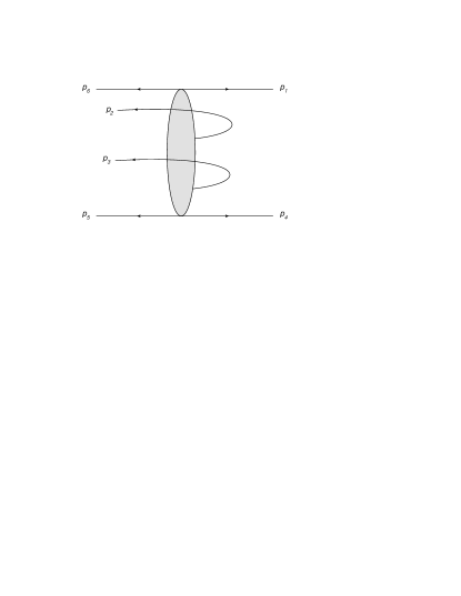
Figure 2: Mandelstam region for $2\to 4$ amplitude.

For the Mandelstam region shown in Fig. 2 the remainder function was first calculated to leading logarithmic accuracy in Ref. BLS2 and given to all orders by,

$$R_{6;MHV}\simeq\frac{ia}{2}\sum_{n=-\infty}^{+\infty}\int_{-\infty}^{+\infty}d\nu\frac{(-1)^{n}}{\nu^{2}+\frac{n^{2}}{4}}w^{i\nu+\frac{n}{2}}(w^{*})^{i\nu-\frac{n}{2}}\left(\left(\frac{s_{45}}{s_{0}}\right)^{-aE_{n,\nu}}-1\right),$$ (6)

where $E_{n,\nu}$ is the eigenvalue of the BFKL equation in the adjoint representation

$$E_{n,\nu}=-\frac{1}{2}\frac{|n|}{\nu^{2}+\frac{n^{2}}{4}}+\psi\left(1+i\nu+\frac{|n|}{2}\right)+\psi\left(1-i\nu+\frac{|n|}{2}\right)-2\psi(1),$$ (7)

where $\psi(z)=\Gamma^{\prime}(z)/\Gamma(z)$ and $a=g^{2}N/8\pi^{2}$. The continuation to the Mandelstam region is $u_{1}=e^{-2\pi i}|u_{1}|$. The expression in eq. (6) predicts the leading log remainder function to any loop order

$$R_{6;MHV}=\sum_{\ell=2}^{\infty}a^{\ell}R^{(\ell)}_{6;MHV}.$$ (8)

At two loops it was calculated in Ref. BLS2 ; Schabinger:2009bb

$$R^{(2)\;LLA}_{6;MHV}=-\frac{i\pi}{2}\log\left(\frac{s_{23}}{s_{0}}\right)\log\left|1+w\right|^{2}\log\left|1+\frac{1}{w}\right|^{2}$$ (9)

and at three loops in Ref. LP2

$$R^{(3)\;LLA}_{6;MHV}=\frac{i\pi}{4}\log^{2}\left(\frac{s_{23}}{s_{0}}\right)\left(\log|w|^{2}\log^{2}|1+w|^{2}-\frac{2}{3}\log^{3}|1+w|^{2}-\frac{1}{4}\log^{2}|w|^{2}\log|1+w|^{2}\;\;\;\right.$$

$$\left.\;\;\;\;+\frac{1}{2}\log|w|^{2}\left(\text{Li}_{2}\left(-w\right)+\text{Li}_{2}\left(-w^{*}\right)\right)-\text{Li}_{3}\left(-w\right)-\text{Li}_{3}\left(-w^{*}\right)\right)$$ (10)

At the leading logarithmic level the energy scale $s_{0}$ is arbitrary and among other possible choices we prefer

$$\frac{s_{23}}{s_{0}}=\frac{1}{\sqrt{u_{2}u_{3}}},$$ (11)

which follows from the requirement of Regge factorization and agreement with next-to-leading corrections at three loops as shown in Ref. FadLip .

In the MHV $2\to 4$ amplitude in Regge kinematics, the helicity of the colliding particles is not changed, which limits the number of the possible helicity configurations to either $++++--$ or $+--+--$ (and their conjugates). In both cases the leading log remainder function is the same. For the NMHV case in MRK one can change a helicity of one of the produced particles $p_{2}$ or $p_{3}$, and it is sufficient to consider only one case, as all other cases are obtained by complex conjugation of the complex $w$ variable. Here we consider in more detail the $++-+--$ helicity configuration, where the produced particle $p_{3}$ has opposite helicity to that of the MHV case. The all orders leading logarithm NMHV remainder function is given by

$$R^{LLA}_{6;NMHV}\simeq-\frac{ia}{2}\sum_{n=-\infty}^{+\infty}\int_{-\infty}^{+\infty}d\nu\frac{(-1)^{n}}{(i\nu+\frac{n}{2})^{2}}w^{i\nu+\frac{n}{2}}(w^{*})^{i\nu-\frac{n}{2}}\left(\left(\frac{s_{23}}{s_{0}}\right)^{-aE_{n,\nu}}-1\right).$$ (12)

Note that eq. (12) can be obtained from eq. (6) by making the following substitution in the integrand

$$\frac{1}{-i\nu+\frac{n}{2}}\rightarrow-\frac{1}{i\nu+\frac{n}{2}},$$ (13)

which follows from the fact that to leading order in MRK the impact factors for gluons with opposite helicities are related by $\chi(\nu,n)\rightarrow\chi^{*}(-\nu,-n)$ (see Appendix A for more details). It also follows from the above property of the impact factors that to the leading logarithmic order

$$\int dw^{*}\frac{w}{w^{*}}\frac{\partial}{\partial w}R_{NMHV}=-R_{MHV}$$ (14)

for the helicity configuration under discussion. The two loop NMHV remainder function in the leading logarithmic approximation is calculated in the Appendix B and given by

$$R^{(2)\;LLA}_{NMHV}\simeq\frac{i\pi}{2}\log\left(\frac{s_{23}}{s_{0}}\right)\left\{\frac{1}{1+w^{*}}\left(\frac{}{}\log|w|^{2}\log(1+w^{*})-\text{Li}_{2}(-w)+\text{Li}_{2}(-w^{*})\right)\right.$$

$$\left.+\frac{1}{1+\frac{1}{w^{*}}}\left(\log\frac{1}{|w|^{2}}\log\left(1+\frac{1}{w^{*}}\right)-\text{Li}_{2}\left(-\frac{1}{w}\right)+\text{Li}_{2}\left(-\frac{1}{w^{*}}\right)\right)\right\}$$ (15)

It is convenient to define the ratio function

$$\mathcal{P}_{NMHV}=\frac{\mathcal{A}^{NMHV}}{\mathcal{A}^{MHV}},$$ (16)

which to leading logarithmic order can be written as

$$\mathcal{P}^{LLA}_{NMHV}\simeq R^{LLA}_{NMHV}-R^{LLA}_{MHV}$$ (17)

From eq. (6) and eq. (12) and the fact that

$$-\frac{1}{(i\nu+\frac{n}{2})^{2}}-\frac{1}{\nu^{2}+\frac{n^{2}}{4}}=-\frac{1}{\nu^{2}+\frac{n^{2}}{4}}\frac{n}{i\nu+\frac{n}{2}}$$ (18)

allows us to write a compact expression for the ratio function in leading logarithmic approximation

$$\mathcal{P}^{LLA}_{6\;NMHV}\simeq-\frac{ia}{2}\sum_{n=-\infty}^{+\infty}\int_{-\infty}^{+\infty}d\nu\frac{(-1)^{n}}{\nu^{2}+\frac{n^{2}}{4}}\frac{n}{i\nu+\frac{n}{2}}w^{i\nu+\frac{n}{2}}(w^{*})^{i\nu-\frac{n}{2}}\left(\frac{s_{23}}{s_{0}}\right)^{-aE_{n,\nu}}.$$ (19)

Note that we dropped the minus unity in the brackets in eq. (12) because, in contrast to the remainder function, the ratio function is well defined also at one loop. This is due to the fact that the divergences at $n=\nu=0$ cancel between the MHV and the NMHV parts resulting in a finite answer also at one loop

$$\mathcal{P}_{6\;NMHV}^{(1)\;LLA} \simeq i\pi\frac{1}{1+w^{*}}\log|1+w|^{2}+i\pi\frac{w^{*}}{1+w^{*}}\log\left|1+\frac{1}{w}\right|^{2}$$

$$=-i\pi\frac{1}{1+w^{*}}\log\tilde{u}_{2}-i\pi\frac{w^{*}}{1+w^{*}}\log\tilde{u}_{3}.\;\;\;$$

At two loops we have

$$\mathcal{P}_{6\;NMHV}^{(2)\;LLA}\simeq\frac{i\pi}{2}\log\left(\frac{s_{23}}{s_{0}}\right)\left\{\frac{1}{1+w^{*}}\left(\frac{}{}\log|w|^{2}\log(1+w^{*})-\text{Li}_{2}(-w)+\text{Li}_{2}(-w^{*})\right)\right.$$

$$\hskip 56.9055pt\left.+\frac{1}{1+\frac{1}{w^{*}}}\left(\log\frac{1}{|w|^{2}}\log\left(1+\frac{1}{w^{*}}\right)-\text{Li}_{2}\left(-\frac{1}{w}\right)+\text{Li}_{2}\left(-\frac{1}{w^{*}}\right)\right)\right\}$$

$$\hskip 56.9055pt+\frac{i\pi}{2}\log\left(\frac{s_{23}}{s_{0}}\right)\log\left|1+w\right|^{2}\log\left|1+\frac{1}{w}\right|^{2}$$ (21)

III NMHV at two loops

In this section we consider the NMHV superamplitude at two loops derived by Dixon, Drummond and Henn in Ref. DixonNMHV . It is convenient to define the ratio function $\mathcal{P}$, which relates all possible helicity configurations of the external particles to the MHV superamplitude

$$\mathcal{A}=\mathcal{A}_{MHV}\times\mathcal{P}.$$ (22)

The expansion of $\mathcal{P}$ in Grassmann variables gives the corresponding type of amplitudes

$$\mathcal{P}=1+\mathcal{P}_{NMHV}+\mathcal{P}_{N^{2}MHV}+...+\mathcal{P}_{\overline{MHV}}.$$ (23)

We focus on the six particle amplitude, where at the tree level the ratio function can be expressed in terms of dual superconformal ”R-invariants” as follows Drummond:2008bq ; Drummond:2008vq

$$\mathcal{P}^{(0)}_{NMHV}=R_{1;35}+R_{1;36}+R_{1;46}.$$ (24)

It is useful to introduce the momentum twistors $Z_{i}$ and supertwistors $\mathcal{Z}_{i}$ Hodges:2009hk

$$\mathcal{Z}_{i}=(Z_{i}|\chi_{i}),\;Z_{i}^{R=\alpha,\dot{\alpha}}=(\lambda_{i}^{\alpha},x_{i}^{\beta\dot{\alpha}}\lambda_{i\beta}),\;\chi_{i}^{A}=\theta_{i}^{\alpha A}\lambda_{i\alpha}$$ (25)

with

$$(abcd)=\epsilon_{RSTU}Z_{a}^{R}Z_{b}^{S}Z_{c}^{T}Z_{d}^{U},$$ (26)

where one defines dual coordinates by

$$p_{i}^{\alpha\dot{\alpha}}=\lambda_{i}^{\alpha}\tilde{\lambda}_{i}^{\dot{\alpha}}=x_{i}^{\alpha\dot{\alpha}}-x_{i+1}^{\alpha\dot{\alpha}},\;\;q_{i}^{\alpha A}=\lambda_{i}^{\alpha}\eta_{i}^{A}=\theta_{i}^{\alpha A}-\theta_{i+1}^{\alpha A}.$$ (27)

The R-invariants can be written compactly in terms of momentum twistors using

$$[abcde]=\frac{\delta^{4}(\chi_{a}(bcde)+cyclic)}{(abcd)(bcde)(cdea)(deab)(eabc)}$$ (28)

and

$$R_{r;ab}=[r,a-1,a,b-1,b].$$ (29)

For the six particle amplitude there are six different invariants. For simplicity one can label them by $(t)$, using the momentum twistor $t$ that is absent from the five arguments in the brackets, e.g.

$$(1)\equiv[23456].$$ (30)

Using the identity between the invariants Drummond:2008vq

$$(1)-(2)+(3)-(4)+(5)-(6)=0$$ (31)

we can write the NMHV amplitude (24) as

$$\mathcal{P}^{(0)}_{NMHV}=(6)+(4)+(2)=(1)+(3)+(5).$$ (32)

The loop contributions are taken into account dressing $(t)$ by functions of the dual conformal invariants $u_{i}$ DixonNMHV

$$\mathcal{P}_{NMHV} =\frac{1}{2}\left\{\frac{}{}\left[(1)+(4)\right]V(u_{1},u_{2},u_{3})+\left[(2)+(5)\right]V(u_{2},u_{3},u_{1})+\left[(3)+(6)\right]V(u_{3},u_{1},u_{2})\right.$$ (33)

$$\left.+\left[(1)-(4)\right]\tilde{V}(y_{1},y_{2},y_{3})-\left[(2)-(5)\right]\tilde{V}(y_{2},y_{3},y_{1})+\left[(3)-(6)\right]\tilde{V}(y_{3},y_{1},y_{2})\right\},$$

where

$$y_{i}=\frac{u_{i}-z_{+}}{u_{i}-z_{-}}$$ (34)

are given by

$$z_{\pm}=\frac{1}{2}\left[-1+u_{1}+u_{2}+u_{3}\pm\sqrt{\Delta}\right],\;\;\;\Delta=(1-u_{1}-u_{2}-u_{3})^{2}-4u_{1}u_{2}u_{3}.$$ (35)

The functions $V$ and $\tilde{V}$ represent parity conserving and parity violating amplitudes respectively and obey the symmetry properties

$$V(u_{3},u_{2},u_{1})=V(u_{1},u_{2},u_{3}),\;\tilde{V}(y_{3},y_{2},y_{1})=-\tilde{V}(y_{1},y_{2},y_{3})$$ (36)

and are functions of the coupling constant

$$V(a)=\sum_{\ell=0}^{\infty}a^{\ell}V^{(\ell)},\;\;\tilde{V}(a)=\sum_{\ell=0}^{\infty}a^{\ell}\tilde{V}^{(\ell)}.$$ (37)

At tree level

$$V^{(0)}=1,\;\tilde{V}^{(0)}=0$$ (38)

and at one loop we have Schabinger:2011kb ; Kosower:2010yk ; Drummond:2008vq ; Schabinger:2011wh

$$V^{(1)}(u_{1},u_{2},u_{3}) =\frac{1}{2}\left[\frac{}{}-\log u_{1}\log u_{3}+\log(u_{1}u_{3})\log u_{2}+\text{Li}_{2}(1-u_{1})\right.$$ (40)

$$\left.\hskip 56.9055pt+\text{Li}_{2}(1-u_{2})+\text{Li}_{2}(1-u_{3})-2\zeta_{2}\frac{}{}\right],$$

$$\tilde{V}^{(1)}(u_{i},u_{j},u_{k})=0,$$

while at two loops both $V^{(2)}$ and $\tilde{V}^{(2)}$ are non-vanishing and were calculated in Ref. DixonNMHV . In the present study we check the analytic properties of $V^{(1)}$, $V^{(2)}$ and $\tilde{V}^{(2)}$ going to the Mandelstam region and show that they correctly reproduce the BFKL calculations to leading logarithmic accuracy.

III.1 Multi-Regge kinematics in the Euclidean region

In this section we consider multi-Regge kinematics of eq. (4) for $2\to 4$ scattering and perform an analytic continuation of $V$ and $\tilde{V}$ to the corresponding Mandelstam region in Fig. 2 reproducing the BFKL leading log calculations at one and two loops.

In multi-Regge kinematics $y_{i}$ are functions of only the complex variables $w$ and $w^{*}$

$$y_{1}\to 1,\;y_{2}\to\tilde{y}_{2}=\frac{1+w^{*}}{1+w},\;y_{3}\to\tilde{y}_{3}=\frac{1+\frac{1}{w}}{1+\frac{1}{w^{*}}}.$$ (41)

Before discussing the Mandelstam region, we investigate the Regge behavior of the function $V$ and $\tilde{V}$ at one loop in the Euclidean region

$$V^{(1)}(u_{1},u_{2},u_{3})\simeq\frac{1}{2}\log u_{2}\log u_{3},$$ (42)

$$V^{(1)}(u_{3},u_{1},u_{2})\simeq-\frac{1}{2}\log u_{2}\log u_{3},$$

$$V^{(1)}(u_{2},u_{3},u_{1})\simeq+\frac{1}{2}\log u_{2}\log u_{3}$$

and two loops

$$V^{(2)}(u_{1},u_{2},u_{3})\simeq\frac{1}{16}\log^{2}u_{2}\log^{2}u_{3},$$ (43)

$$V^{(2)}(u_{3},u_{1},u_{2})\simeq-\frac{1}{16}\log^{2}u_{2}\log^{2}u_{3},$$

$$V^{(2)}(u_{2},u_{3},u_{1})\simeq\frac{1}{16}\log^{2}u_{2}\log^{2}u_{3}$$

$$\tilde{V}^{(2)}(y_{i},y_{j},y_{k})\simeq 0.$$

We immediately notice a very disturbing feature of $V$, namely, that they are badly divergent in the MRK of eq. (4) because

$$\log u_{2}\log u_{3}\simeq\log^{2}\delta+\log\delta\log(\tilde{u}_{2}\tilde{u}_{3})+\mathcal{O}(1),$$ (44)

where (see also eq. (11))

$$\delta=\sqrt{u_{2}u_{3}}=(1-u_{1})\sqrt{\tilde{u_{2}}\tilde{u_{3}}}\to 0$$ (45)

is the only small parameter along with finite $\tilde{u}_{2}$ and $\tilde{u}_{3}$. From Regge theory we expect all such divergences in the Euclidean region to cancel between them. This implies the condition

$$[(1)+(4)]+[(2)+(5)]-[(3)+(6)]=0,$$ (46)

which we check later by explicit calculation of the R-invariant in eq. (28). The function $\tilde{V}$ is zero at one loop and vanishing at two loops in MRK

III.2 The Mandelstam Region

We consider the Mandelstam region illustrated in Fig. 2, where we flip two produced particles. The analytic continuation for the $2\to 4$ scattering, which takes one from the Euclidean region to the Mandelstam region is given by

$$u_{1}=|u_{1}|e^{-i2\pi},\;u_{2}=|u_{2}|,\;u_{3}=|u_{3}|.$$ (47)

After the analytic continuation eq. (47) the functions $V$ at one loop in MRK read

$$V^{(1)}(u_{1},u_{2},u_{3})\rightarrow V^{(1)}(u_{1},u_{2},u_{3})+i\pi\log\delta-\frac{i3\pi}{2}\log\tilde{u}_{2}+\frac{i\pi}{2}\log\tilde{u}_{3}$$ (48)

$$V^{(1)}(u_{3},u_{1},u_{2})\rightarrow V^{(1)}(u_{3},u_{1},u_{2})-i\pi\log\delta+\frac{i\pi}{2}\log\tilde{u}_{2}-\frac{i\pi}{2}\log\tilde{u}_{3}$$

$$V^{(1)}(u_{2},u_{3},u_{1})\rightarrow V^{(1)}(u_{2},u_{3},u_{1})+i\pi\log\delta+\frac{i\pi}{2}\log\tilde{u}_{2}-\frac{i3\pi}{2}\log\tilde{u}_{3}.$$

We note that the cancelation of undesired $i\pi\log\delta$ terms is guaranteed by the condition eq. (46) on the R-invariants. Indeed, projecting $(t)$ onto the $++-+--$ helicity configuration, relevant for $2\to 4$ scattering in the multi-Regge kinematics, we obtain

$$(1)\rightarrow\frac{1}{1+w^{*}},\;(5)\rightarrow\frac{w^{*}}{1+w^{*}},\;(6)\rightarrow 1,\;(2)\rightarrow 0,\;(3)\rightarrow 0,\;(4)\rightarrow 0,$$ (49)

which agrees with the condition for the cancelation of large logarithms in eq. (46). Inserting eq. (49) in the ratio function $\mathcal{P}$ in eq. (33) at tree level we get $\mathcal{P}=1$ and at one loop we reproduce the BFKL result of eq. (II.2), namely

$$\mathcal{P}_{6\;NMHV}^{(1)\;LLA} \simeq -i\pi\frac{1}{1+w^{*}}\log\tilde{u}_{2}-i\pi\frac{w^{*}}{1+w^{*}}\log\tilde{u}_{3}.\;\;\;$$ (50)

At two loops the analytic continuation of $V$ and $\tilde{V}$ is performed using the prescription for the symbol introduced in Ref. Dixon3loops . The relative simplicity of the symbol after the analytic continuation allows us to find a corresponding function up to possible ”non-pure” functions, such as $\zeta_{2}$ or those are built of powers of $\pi$ times pure functions, and thus are beyond the accuracy of the leading logarithmic approximation considered in the present study. Each individual $V$ contains undesired large logarithm terms of the order $i\pi\log^{3}\delta$, but those cancel in sum leaving only reasonable subleading logarithmic terms of the order $i\pi\log^{\ell-1}\delta$ ($\ell$ is the number of loops). The functions $\tilde{V}$ have only ”good” leading log terms and thus we have

$$V^{(2)}(u_{1},u_{2},u_{3})+V^{(2)}(u_{3},u_{1},u_{2}) \rightarrow-\frac{i\pi}{2}\log\delta\log^{2}\tilde{u}_{2}-\frac{i\pi}{2}\log\delta\log\tilde{u}_{2}\log\tilde{u}_{3}+\mathcal{O}(1),$$ (51)

$$V^{(2)}(u_{2},u_{3},u_{1})+V^{(2)}(u_{3},u_{1},u_{2}) \rightarrow-\frac{i\pi}{2}\log\delta\log^{2}\tilde{u}_{3}-\frac{i\pi}{2}\log\delta\log\tilde{u}_{2}\log\tilde{u}_{3}+\mathcal{O}(1),$$

$$\tilde{V}^{(2)}(y_{1},y_{2},y_{3})\rightarrow i\pi\log\delta\left(\frac{1}{2}\log|w|^{2}\log\frac{1+w}{1+w^{*}}+\text{Li}_{2}(-w)-\text{Li}_{2}(-w^{*})\right)+\mathcal{O}(1).$$

Inserting eq. (51) and eq. (49) into the expression for the ratio function in eq. (33) we get

$$\mathcal{P}_{6\;NMHV}^{(2)\;LLA} =\frac{1}{2}\frac{1}{1+w^{*}}\left(\frac{}{}V^{(2)}(u_{1},u_{2},u_{3})+V^{(2)}(u_{3},u_{1},u_{2})+\tilde{V}^{(2)}(y_{1},y_{2},y_{3})-\tilde{V}^{(2)}(y_{3},y_{1},y_{2})\right)$$ (52)

$$+\frac{1}{2}\frac{w^{*}}{1+w^{*}}\left(\frac{}{}V^{(2)}(u_{2},u_{3},u_{1})+V^{(2)}(u_{3},u_{1},u_{2})+\tilde{V}^{(2)}(y_{2},y_{3},y_{1})-\tilde{V}^{(2)}(y_{3},y_{1},y_{2})\right)\;\;\;\;$$

$$\simeq-\frac{i\pi}{2}\log\delta\left\{\frac{1}{1+w^{*}}\left(\frac{}{}-\log|w|^{2}\log(1+w)+\log^{2}|1+w|^{2}-\text{Li}_{2}(-w)+\text{Li}_{2}(-w^{*})\right)\right.$$

$$\left.+\frac{1}{1+\frac{1}{w^{*}}}\left(-\log\frac{1}{|w|^{2}}\log\left(1+\frac{1}{w}\right)+\log^{2}\left|1+\frac{1}{w}\right|^{2}-\text{Li}_{2}\left(-\frac{1}{w}\right)+\text{Li}_{2}\left(-\frac{1}{w^{*}}\right)\right)\right\}$$

which reproduces the BFKL result in eq. (II.2). The overall minus sign is due to the fact that $\log(s_{23}/s_{0})=-\log\delta$.

It is worth emphasizing that the first two lines of eq. (52) represent a general structure valid to any loop order in the leading logarithm approximation. It is unambiguously fixed by properties of $V$ and $\tilde{V}$ in eq. (36), the target-projectile symmetry as well as the proper collinear limit as follows. In the multi-Regge kinematics of eq. (4) the variables $u_{i}$ and $y_{i}$ can be written as

$$u_{1}\to 1,\;u_{2}\to\frac{1-u_{1}}{|1+w|^{2}},\;u_{3}\to\frac{1-u_{1}}{|1+\frac{1}{w}|^{2}},\;y_{1}\to 1,\;y_{2}\to\frac{1+w^{*}}{1+w},\;y_{3}\to\frac{1+\frac{1}{w}}{1+\frac{1}{w^{*}}}.$$ (53)

The target-projectile symmetry means that the result is invariant under an exchange of the colliding particles in Fig. 2, which implies $w\leftrightarrow 1/w^{*}$ and thus

$$u_{1}\leftrightarrow u_{1},\;u_{2}\leftrightarrow u_{3},\;y_{2}\leftrightarrow y_{3}.$$ (54)

This fixes the combination of $V$ and $\tilde{V}$ in the brackets in eq. (52), but leaves some freedom of assigning this combination to either $1/(1+w^{*})$ or $1/(1+\frac{1}{w^{*}})$. It is resolved by demanding of a proper collinear limit, i.e. any function which multiplies $1/(1+w^{*})$ should vanish for $|w|\to 0$. The overall coefficient is fixed by the tree level expression. The above arguments are valid to any loop order determining the general structure of the first two lines in eq. (52) for $++-+--$ helicity configuration.

In a similar way we checked the other $+-++--$ helicity configuration for the $2\to 4$ amplitude as well, and found the analytic continuation of $V$ and $\tilde{V}$ to be consistent with BFKL calculations for the $3\to 3$ amplitude for helicity configurations $+++---$, $+-+-+-$ and their conjugates. In the leading logarithm approximation the $3\to 3$ case differs from the $2\to 4$ case only by the sign

$$\mathcal{P}^{LLA}_{2\to 4\;NMHV}=-\mathcal{P}^{LLA}_{3\to 3\;NMHV}=\mathcal{P}^{LLA}_{6\;NMHV}$$ (55)

for $\mathcal{P}^{LLA}_{6\;NMHV}$ in eq. (19). The same is true also for the MHV and NMHV remainder functions.

The analytic continuation to the Mandelstam region for the $3\to 3$ amplitude is given by BLP3to3 ; BLS2

$$u_{1}=|u_{1}|e^{i2\pi},\;u_{2}=|u_{2}|e^{-i\pi},\;u_{3}=|u_{3}|e^{-i\pi}$$ (56)

and the multi-Regge kinematics reads

$$u_{1}\to 1^{+},\;u_{2}\to 0^{+},\;u_{3}\to 0^{+},\;\text{with}\;\;\tilde{u}_{2}=\left|\frac{u_{2}}{1-u_{1}}\right|\simeq\mathcal{O}(1)\;\text{and}\;\tilde{u}_{3}=\left|\frac{u_{3}}{1-u_{1}}\right|\simeq\mathcal{O}(1).$$ (57)

Note that in the $3\to 3$ case $1-u_{1}$ is negative resulting in the difference of the real part between $3\to 3$ and $2\to 4$ remainder functions as discussed in the next section.

Using the property in eq. (14) and the three loop remainder function in eq. (II.2) we calculate the three loop leading log remainder function in eq. (12)

$$R^{(3)\;LLA}_{6;NMHV} \simeq\frac{i\pi}{4}\log^{2}\delta\left(\frac{1}{1+w^{*}}f_{3}(w,w^{*})+\frac{1}{1+\frac{1}{w^{*}}}f_{3}\left(\frac{1}{w},\frac{1}{w^{*}}\right)\right),$$ (58)

where

$$f_{3}(w,w^{*})= -\frac{1}{2}\log^{2}|w|^{2}\log(1+w^{*})+\log(-w)\left(\log^{2}(1+w^{*})-\log^{2}(1+w)\frac{}{}\right)$$

$$+2\zeta_{2}\log|1+w|^{2}+\frac{1}{2}\log|w|^{2}\left(\text{Li}_{2}(-w)-\text{Li}_{2}(-w^{*})\frac{}{}\right)$$

$$-2\log|1+w|^{2}\text{Li}_{2}(-w)-2\text{Li}_{3}(1+w)-2\text{Li}_{3}(1+w^{*})+4\zeta_{3}.$$

The leading log ratio function is then found from eq. (II.2) and eq. (17)

$$\mathcal{P}^{(3)}_{6\;NMHV}\simeq R^{(3)\;LLA}_{6;NMHV}-R^{(3)\;LLA}_{6;MHV}$$ (60)

There is an ambiguity related to the indefinite integral in eq. (14), which is resolved by demanding the singlevaluedness and proper collinear behavior of $R^{(3)\;LLA}_{NMHV}$ (see Appendix B for more details).

Eqs. (58)-(60) present a prediction to be checked against an eventual 3-loop calculation of $V^{(3)}$ and $\tilde{V}^{(3)}$.

IV Real part of the remainder function

In this section we calculate the real part of the remainder function at the next-to-leading logarithm order. The leading logarithm contribution to the remainder function is pure imaginary, of the order $\log^{\ell-1}\delta$ ($\ell$ is the number of loops) and comes entirely from the Mandelstam cut. The real part appears only at the next-to-leading logarithm level of the order of $\log^{\ell-2}$ and originates from both Mandelstam cuts and Regge poles as it was shown in Ref. LipDisp . There is no full separation between poles and cuts in the remainder function due to the fact that the BDS amplitude, lacking the entire contributions from Mandelstam cuts, still has some residual terms which can be assigned to Mandelstam cuts. Those are removed from the remainder function by introducing a phase $\Delta$ extracted from the BDS amplitude at one loop

$$\Delta=\frac{\gamma_{K}}{8}\log\tilde{u}_{2}\tilde{u}_{3}=\frac{\gamma_{K}}{8}\log\frac{|w|^{2}}{|1+w|^{4}},$$ (61)

where $\gamma_{K}\simeq 4a$ and $a=g^{2}N_{c}/8\pi^{2}$ are the cusp anomalous dimension and the coupling constant respectively. Thus one can write LipDisp ; LP2 the dispersion relation for the real and imaginary part of the remainder function for the $2\to 4$ amplitude

$$e^{i\pi\Delta}R_{2\to 4}=\cos\pi\omega_{ab}+i\int_{-i\infty}^{+i\infty}\frac{d\omega}{2\pi i}f(\omega)e^{-i\pi\omega}|\delta|^{-\omega}$$ (62)

and the $3\to 3$ scattering

$$e^{-i\pi\Delta}R_{3\to 3}=\cos\pi\omega_{ab}-i\int_{-i\infty}^{+i\infty}\frac{d\omega}{2\pi i}f(\omega)|\delta|^{-\omega}.$$ (63)

The phase $\Delta$ removes the residual cut terms of the BDS amplitude from the remainder function and the last term in eq. (62) and eq. (63) restores the correct Mandelstam cut contribution. The Regge poles are accounted for by the $\cos\pi\omega_{ab}$ term with

$$\omega_{ab}=\frac{\gamma_{K}}{8}\log\frac{\tilde{u}_{3}}{\tilde{u}_{2}}=\frac{\gamma_{K}}{8}\log|w|^{2}.$$ (64)

To the leading logarithm order for the MHV amplitude the function $f(\omega)$ is determined from eq. (6) as

$$i\int_{-i\infty}^{+i\infty}\frac{d\omega}{2\pi i}f^{LLA}_{MHV}(\omega)|\delta|^{-\omega}=\frac{ia}{2}\sum_{n=-\infty}^{+\infty}\int_{-\infty}^{+\infty}d\nu\frac{(-1)^{n}}{\nu^{2}+\frac{n^{2}}{4}}w^{i\nu+\frac{n}{2}}(w^{*})^{i\nu-\frac{n}{2}}\delta^{aE_{n,\nu}},$$ (65)

and the next-to-leading corrections to $f(\omega)$ were found in Refs. LP2 ; FadLip . The phase coefficient $e^{-i\pi\omega}$ in the integrand of eq. (62) makes the real part of remainder function to obtain contributions from the imaginary part substituting

$$\log\delta\to\log\delta+i\pi$$ (66)

in the leading logarithm terms of the same loop order, whereas the phase $\Delta$ gives the contribution to the real part from the imaginary leading logarithm terms of the previous loop order. For example, expanding eq. (62) to the second order in $a$ one obtains

$$a^{2}\Re\left(R^{(2);NLLA}_{2\to 4;\;MHV}\right)\simeq-i\pi\Delta R^{(1);LLA}_{2\to 4;\;MHV}-\frac{\pi^{2}\omega^{2}_{ab}}{2}+\frac{\pi^{2}\delta^{2}}{2}+R^{(2);LLA}_{2\to 4;\;MHV}|_{\log\delta\to i\pi}\simeq 0$$ (67)

provided the one loop remainder function $R^{(1);LLA}_{2\to 4;\;MHV}$ is set to be zero. In eq. (67) the Regge pole and Mandelstam cut contributions cancel out resulting in the zero real part for the MHV remainder at two loops for the $2\to 4$ scattering amplitude. For the $3\to 3$ case in eq. (63) the mixing phase $e^{-i\pi\omega}$ is absent in the integrand, and thus we have a non-vanishing real part

$$a^{2}\Re\left(R^{(2);NLLA}_{3\to 3;\;MHV}\right)\simeq-i\pi\Delta R^{(1);LLA}_{3\to 3;\;MHV}-\frac{\pi^{2}\omega^{2}_{ab}}{2}+\frac{\pi^{2}\delta^{2}}{2}=\frac{\pi^{2}}{2}\log|1+w|^{2}\log\left|1+\frac{1}{w}\right|^{2}.\;\;\;$$ (68)

The absence of $e^{-i\pi\omega}$ in eq. (63) allows us to make all loop prediction for the following object BLP3to3

$$\Re\left(e^{-i\pi\Delta}R_{3\to 3}\right)=\cos\pi\omega_{ab},$$ (69)

which is valid also in the strong coupling region.

The dispersion relations eq. (62) and eq. (63) remain valid also for the NMHV remainder functions, because in the derivation no assumption was made about the helicity configuration of the produced particles. The real part of the $2\to 4$ next-to-leading ratio function is given by

$$\Re(\mathcal{P}_{2\to 4}^{NLLA}) \simeq-i\pi\Delta\mathcal{P}_{2\to 4}^{LLA}+\mathcal{P}_{2\to 4}^{LLA}|_{\log\delta\to\log\delta+i\pi}-\mathcal{P}_{2\to 4}^{LLA}$$

$$\simeq-i\pi\Delta\mathcal{P}_{6}^{LLA}+\mathcal{P}_{6}^{LLA}|_{\log\delta\to\log\delta+i\pi}-\mathcal{P}_{6}^{LLA},\;\;\;$$

and for $3\to 3$ scattering it reads

$$\Re(\mathcal{P}_{3\to 3}^{NLLA})\simeq i\pi\Delta\mathcal{P}_{3\to 3}^{LLA}\simeq-i\pi\Delta\mathcal{P}_{6}^{LLA}$$ (71)

for the leading logarithm ratio function $\mathcal{P}_{6}^{LLA}$ in eq. (19). The contributions of the Regge poles $\cos\omega_{ab}$ completely cancel out in the ratio function having the same sign in eq. (67) and eq. (68).

The last two terms in eq. (IV) can be written as

$$\mathcal{P}_{6}^{LLA}|_{\log\delta\to\log\delta+i\pi}-\mathcal{P}_{6}^{LLA}\simeq\frac{a^{2}\pi}{2}\sum_{n=-\infty}^{+\infty}\int_{-\infty}^{+\infty}d\nu\frac{(-1)^{n}}{\nu^{2}+\frac{n^{2}}{4}}\frac{n}{i\nu+\frac{n}{2}}w^{i\nu+\frac{n}{2}}(w^{*})^{i\nu-\frac{n}{2}}E_{n,\nu}\;\delta^{aE_{n,\nu}}.$$ (72)

We checked that the $V$ and $\tilde{V}$ of Ref. DixonNMHV correctly reproduce the real parts of the $2\to 4$ and $3\to 3$ remainder functions at two loops. Expressions in eq. (IV) and eq. (71) together with eqs. (52)-(60) give a prediction for the next-to-leading real part of the remainder at three loops.

V More legs

In this section we consider N^kMHV in the leading log approximation with more external gluons. We start our discussion with the $2\to 5$ amplitude, where we have three produced particles with momenta $p_{2}$, $p_{3}$ and $p_{4}$. In multi-Regge kinematics the number of possible helicity configurations is limited due to the fact that the colliding particles have eikonal vertices and as a result their helicities stay the same. In the convention where all momenta are outgoing this implies that helicities of particles with $p_{1}$ and $p_{7}$ should have opposite sign, and the same for gluons with $p_{5}$ and $p_{6}$. The helicities of the produced particles with momenta $p_{4}$, $p_{5}$ and $p_{6}$ are arbitrary. The $2\to 5$ MHV amplitude was considered in Ref. Bartels25 ; Prygarin:2011gd and it was shown that its leading log remainder function can be written as a sum of two $2\to 4$ remainder functions. This happens due to some cancelations between propagators and effective vertices for particles of the same helicity. Unfortunately this is not the case with NMHV amplitudes, but one can consider Mandelstam regions, where only two adjacent particles are flipped and then the remainder function is given by the same expression as for $2\to 4$ case in eq. (12) with redefined $s_{23}/s_{0}$ and $w$.

Figure 3: One of the Mandelstam regions for $2\to 5$ amplitude in which the remainder function reduces to the $2\to 4$ case with redefined momenta.

For example, when we flip produced particles with momenta $p_{2}$ and $p_{3}$ as depicted in Fig. 3 for $++-++--$ helicity configuration we get

$$R^{LLA;+-}_{7;2;NMHV}\simeq-\frac{ia}{2}\sum_{n=-\infty}^{+\infty}\int_{-\infty}^{+\infty}d\nu\frac{(-1)^{n}}{(i\nu+\frac{n}{2})^{2}}w^{\prime i\nu+\frac{n}{2}}(w^{\prime*})^{i\nu-\frac{n}{2}}\left(\left(\frac{s_{45}}{s^{\prime}_{0}}\right)^{-aE_{n,\nu}}-1\right),$$ (73)

where the cross ratios are as in eq. (2), but with $i=1$ to $7$;

$$\frac{s_{23}}{s^{\prime}_{0}}=\frac{1}{\sqrt{u_{6}u_{7}}},$$ (74)

and

$$w^{\prime}\equiv\frac{(p_{5}+p_{6})p_{2}}{(p_{7}+p_{1})p_{3}}=\frac{1-\tilde{u}_{6}-\tilde{u}_{7}+\sqrt{(1-\tilde{u}_{6}-\tilde{u}_{7})^{2}-4\tilde{u}_{6}\tilde{u}_{7}}}{2\tilde{u}_{6}}$$ (75)

for

$$\tilde{u}_{1}=\frac{u_{6}}{1-u_{1}},\;\;\tilde{u}_{7}=\frac{u_{7}}{1-u_{1}}.$$ (76)

The multi-Regge kinematics for $2\to 5$ scattering implies

$$1-u_{1}\propto\delta,\;1-u_{2}\propto\delta,\;1-u_{5}\propto\delta^{2},\;\delta\to 0$$ (77)

and the rest of cross ratios are of the order of $\delta$.

In this case the ratio function to leading log accuracy is given by

$$\mathcal{P}^{LLA;+-}_{7;2;NMHV}\simeq-\frac{ia}{2}\sum_{n=-\infty}^{+\infty}\int_{-\infty}^{+\infty}d\nu\frac{(-1)^{n}}{\nu^{2}+\frac{n^{2}}{4}}\frac{n}{i\nu+\frac{n}{2}}w^{\prime i\nu+\frac{n}{2}}(w^{\prime*})^{i\nu-\frac{n}{2}}\left(\frac{s_{23}}{s^{\prime}_{0}}\right)^{-aE_{n,\nu}}.$$ (78)

The corresponding analytic continuation reads

$$u_{1}=|u_{1}|e^{-i2\pi},\;u_{3}=|u_{3}|e^{-i\pi},\;u_{4}=|u_{4}|e^{+i\pi},$$ (79)

while the other cross ratios remain the same.

In a similar way we can find the ratio function for many other Mandelstam regions, where only two adjacent particles are flipped. The problem reduces to a proper redefinition of the energy scale $s_{0}$, the complex variable $w$ and the analytic continuation done case by case.

The NMHV superamplitudes for $n=7$ were considered in Refs. Bern:2004ky ; Drummond:2008bq ; Korchemsky:2009hm , which can be analyzed analogously to that of $n=6$. This is a project for future work. It worth emphasizing that the ratio function for the Mandelstam regions, where we flip two adjacent particles, in the leading order does not depend on the helicities of the all other particles. More detailed discussion on this topic will be presented by us elsewhere.

VI Conclusions

The multi-Regge limit (MRK) for N=4 SYM NMHV amplitudes were considered in two different formulations: the BFKL formalism for multi-Regge amplitudes in leading logarithm approximation, and superconformal N=4 SYM amplitudes. It was shown that the two approaches agreed in explicit calculations in leading logarithm approximation to two loops for the six-point gluon amplitudes. Predictions were made for three loop six point NMHV amplitudes and two-loop seven-point NMHV amplitudes in leading logarithm approximation from the BFKL point of view. Comparisons with similar calculations from superconformal amplitudes should strengthen the connection between these two methods. Another approach to computing the remainder functions is that of the operator product expansion (OPE) developed by Alday, Gaiotto, Maldacena, Sever, and Vieira (AGMSV) Alday:2010ku ; Gaiotto:2011dt ; Sever:2011pc ; Gaiotto:2010fk . In particular Sever, Vieira, and Wang Sever:2011da rederive the one-loop NMHV six-point amplitudes from the OPE point of view. There appears to be a connection between the OPE methods and the BFKL results when compared in the collinear, multi-Regge limits as shown in Ref. Bartels:2011xy . It would be interesting to find the precise relationship between the two points of view, as this could offer additional insights into this class of problems.

After this paper was posted Dixon, Duhr and Pennington Dixon:2012yy presented an extension of the $2\rightarrow 4$ MHV and NMHV amplitudes in the MRK limit to 10-loops using single-valued harmonic polylogarithms as a basis. They confirm the results of this paper.

VII Acknowledgements

We thank J. Bartels, S. Caron-Huot, L. Dixon, V. S. Fadin, J. Henn, G. P. Korchemsky, A. Kormilitzin, E. M. Levin, A. Sever, M. Spradlin, C. -I Tan, C. Vergu and A. Volovich for helpful discussions. The work of AP is supported in part by the the US National Science Foundation under Grant PHY-064310 PECASE. The research of HJS is supported in part by the Department of Energy under Grant DE-FG02-92ER40706.

Appendix A Impact Factors in the BFKL Approach

In this section we find the leading order impact factor needed for calculating the NMHV amplitude in leading logarithm approximation. We adopt the momenta convention of Ref. BLS2 because our analysis is tightly related to discussion presented in Chapters 2 and 5 of Ref. BLS2 . Firstly we note that the effective production vertex $C_{\mu}(\mathbf{q}_{2},\mathbf{q}_{1})$ can be written in a very compact way for a definite helicity of the produced particles

$$C_{\mu}(\mathbf{q}_{2},\mathbf{q}_{1})e_{\mu}(\mathbf{k}_{1})=\sqrt{2}\frac{q_{2}q^{*}_{1}}{k_{1}},$$ (A.1)

where we introduce the complex transverse momenta

$$k=k_{x}+ik_{y},\;\;k^{*}=k_{x}-ik_{y}.$$ (A.2)

Following the lines of Chapter 2 of Ref. BLS2 we readily find that the impact factors for the opposite helicities are related by complex conjugation in momentum space (see eq. (13) of Ref. BLS2 ) and thus we have

$$\Phi^{+}_{2}=\frac{k_{2}(k^{{}^{\prime}}-q_{2})}{q_{2}(k^{{}^{\prime}}-k_{2})},\;\;\Phi^{-}_{2}=\frac{k^{*}_{2}(k^{*^{\prime}}-q^{*}_{2})}{q^{*}_{2}(k^{*^{\prime}}-k^{*}_{2})}.$$ (A.3)

The impact factor has to be convolved with the BFKL Green function (see eqs. (84)-(92) of Ref. BLS2 )

$$\chi^{\pm}_{2}=\int\frac{d^{2}k^{\prime}}{2\pi}\frac{|q_{2}|^{2}}{|k^{\prime}|^{2}|q_{2}-k^{\prime}|^{2}}\left(\frac{q_{2}-k^{\prime}}{k^{\prime}}\right)^{i\nu+\frac{n}{2}}\left(\frac{q^{*}_{2}-k^{*^{\prime}}}{k^{*^{\prime}}}\right)^{i\nu-\frac{n}{2}}\Phi^{\pm}_{2}.$$ (A.4)

It is easy to see from eq. (A.4) that the impact factors for different helicities are related by

$$\chi^{-}(\nu,n)=(\chi^{+}(-\nu,-n))^{*}$$ (A.5)

rather than a simple conjugation. The $\chi_{2}^{+}$ in eq. (A.4) was calculated in Ref. BLS2

$$\chi_{2}^{+}=-\frac{1}{2}\frac{1}{i\nu-\frac{n}{2}}\left(\frac{q_{3}^{*}}{k_{2}^{*}}\right)^{i\nu-\frac{n}{2}}\left(\frac{q_{3}}{k_{2}}\right)^{i\nu+\frac{n}{2}}$$ (A.6)

and eq. (A.5) implies eq. (13) resulting in difference of the integral representations of the leading logarithm MHV and NMHV remainder functions in eq. (6) and eq. (12) respectively.

Appendix B Leading Logarithm NMHV Remainder Functions at One, Two and Three Loops

In this section we calculate the leading logarithm ratio function in eq. (19) given by

$$\mathcal{P}^{LLA}_{6\;NMHV}\simeq-\frac{ia}{2}\sum_{n=-\infty}^{+\infty}\int_{-\infty}^{+\infty}d\nu\frac{(-1)^{n}}{\nu^{2}+\frac{n^{2}}{4}}\frac{n}{i\nu+\frac{n}{2}}w^{i\nu+\frac{n}{2}}(w^{*})^{i\nu-\frac{n}{2}}\left(\frac{s_{23}}{s_{0}}\right)^{-aE_{n,\nu}}.$$ (B.1)

In contrast to the remainder function for the NMHV amplitude in eq. (12), the ratio function is finite even at one loop because the IR divergences cancel between the MHV and NMHV remainder functions. Technically, the divergence of the type $\int d\nu/\nu^{2}$ is absent here due to the presence of $n$ in the numerator, which makes the whole expression to vanish at $n=0$.

We start with the one loop case

$$\mathcal{P}^{(1)\;LLA}_{6\;NMHV}\simeq-\frac{i}{2}\sum_{n=-\infty}^{+\infty}\int_{-\infty}^{+\infty}d\nu\frac{(-1)^{n}}{\nu^{2}+\frac{n^{2}}{4}}\frac{n}{i\nu+\frac{n}{2}}w^{i\nu+\frac{n}{2}}(w^{*})^{i\nu-\frac{n}{2}}$$ (B.2)

and calculate $\mathcal{P}^{(1)\;LLA}_{6\;NMHV}$ using the Cauchy theorem as follows. We assume $|w|>1$ and close the integration contour in the upper semiplane. Then we have poles at $\nu=in/2$ for which $n>0$, and poles at $\nu=-in/2$ for which $n<0$. The residues at poles $\nu=in/2$ give

$$-i\pi\sum_{n=1}^{\infty}\frac{(w^{*})^{-n}}{n}(1+n\log|w|^{2})=i\pi\log(1+w^{*})+\frac{i\pi}{1+w^{*}}\log w-\frac{i\pi\;w^{*}}{1+w^{*}}\log w^{*},$$ (B.3)

while from poles at $\nu=-in/2$ we have

$$i\pi\sum_{n=-\infty}^{-1}\frac{w^{n}}{n}=i\pi\log\left(1+\frac{1}{w}\right).$$ (B.4)

Adding the two contributions we have

$$\mathcal{P}_{6\;NMHV}^{(1)\;LLA} \simeq i\pi\frac{1}{1+w^{*}}\log|1+w|^{2}+i\pi\frac{w^{*}}{1+w^{*}}\log\left|1+\frac{1}{w}\right|^{2}.$$ (B.5)

We notice that $\mathcal{P}_{6\;NMHV}^{(1)\;LLA}$ can be written as

$$\mathcal{P}_{6\;NMHV}^{(1)\;LLA} \simeq \frac{i\pi}{1+w^{*}}\tilde{f}_{1}(w,w^{*})+\frac{i\pi}{1+\frac{1}{w^{*}}}\tilde{f}_{1}\left(\frac{1}{w},\frac{1}{w^{*}}\right),$$ (B.6)

where

$$\tilde{f}_{1}(w,w^{*})=\log|1+w|^{2}.$$ (B.7)

The functions $1/(1+w^{*})$ and $1/(1+\frac{1}{w^{*}})$ are related to $R$-invariants and are universal for all loops. Thus the problem of calculating the ratio function reduces to finding $\tilde{f}_{\ell}(w,w^{*})$, where $\ell$ is the number of loops. By virtue of eq. (17), the function $\tilde{f}_{\ell}(w,w^{*})$ includes the MHV remainder function and it is useful to introduce a redefined function $f_{\ell}(w,w^{*})$ defined by

$$f_{\ell}(w,w^{*})=\tilde{f}_{\ell}(w,w^{*})-f^{MHV}_{\ell}(w,w^{*}),$$ (B.8)

where $f^{MHV}_{\ell}(w,w^{*})$ is the corresponding MHV contribution. The function $f_{\ell}(w,w^{*})$ can be found from $f^{MHV}_{\ell}(w,w^{*})$ using the property of the leading logarithm NMHV remainder functions in eq. (14)

$$R_{NMHV}=-\int dw\frac{w^{*}}{w}\frac{\partial}{\partial w^{*}}R_{MHV}$$ (B.9)

and demanding singlevaluedness and proper collinear behavior. At two loops we read out from eq. (9)

$$f^{MHV}_{2}(w,w^{*})=\log|1+w|^{2}\log\left|1+\frac{1}{w}\right|^{2}$$ (B.10)

and then using eq. (B.9) obtain

$$-\int dw\frac{w^{*}}{w}\frac{\partial}{\partial w^{*}}f^{MHV}_{2}(w,w^{*}) =\frac{1}{1+w^{*}}\left(\log|w|^{2}\log(1+w^{*})-\frac{1}{2}\log^{2}(1+w^{*})-\text{Li}_{2}(-w)\right)$$ (B.11)

$$+\frac{w^{*}}{1+w^{*}}\left(\frac{1}{2}\log^{2}w+\log w^{*}\log w-\log w\log(1+w^{*})+\text{Li}_{2}(-w)\right)+F(w^{*}),\;\;\;\;$$

where $F(w^{*})$ is some arbitrary function of only $w^{*}$. We fix $F(w^{*})$ by demanding singlevaluedness for $w$ being rotated by an arbitrary phase $\phi$ and $w^{*}$ rotated by $-\phi$. The best way to see how this determines $F(w^{*})$ is to inspect the first term in eq. (B.11), namely the function

$$\log|w|^{2}\log(1+w^{*})-\frac{1}{2}\log^{2}(1+w^{*})-\text{Li}_{2}(-w).$$ (B.12)

Its symbol reads

$$w\otimes(1+w^{*})+(1+w)\otimes w+w^{*}\otimes(1+w^{*})+(1+w^{*})\otimes w$$ (B.13)

$$+(1+w^{*})\otimes w^{*}-(1+w^{*})\otimes(1+w^{*}),$$

and the analytic continuation is done clipping the first entry Dixon3loops . In particular, for $w<1$

$$w\otimes(1+w^{*})\rightarrow w\otimes(1+w^{*})+i\phi\;(1+w^{*})$$ (B.14)

and the last term cancels in eq. (B.13) against

$$w^{*}\otimes(1+w^{*})\rightarrow w^{*}\otimes(1+w^{*})-i\phi\;(1+w^{*}).$$ (B.15)

For $w>1$ we have also

$$(1+w)\otimes w\rightarrow(1+w)\otimes w+i\phi\;w+\frac{(i\phi)^{2}}{2}$$ (B.16)

and the last two terms cancel against

$$(1+w^{*})\otimes w\rightarrow(1+w^{*})\otimes w-i\phi\;w-\frac{(i\phi)^{2}}{2}.$$ (B.17)

This cancelation does not happen for $(1+w^{*})\otimes w^{*}$ and $-(1+w^{*})\otimes(1+w^{*})$ in eq. (B.13), and we can use the freedom of choosing $F(w^{*})$ to remove those. Thus we are left with

$$w\otimes(1+w^{*})+(1+w)\otimes w+w^{*}\otimes(1+w^{*})+(1+w^{*})\otimes w,$$ (B.18)

which matches

$$f_{2}(w,w^{*})=\log|w|^{2}\log(1+w^{*})-\text{Li}_{2}(-w)+\text{Li}_{2}(-w^{*})$$ (B.19)

up to a constant, which can be shown to be zero by demanding eq. (B.18) to be vanishing as $|w|\to 0$ in the collinear limit. Now we readily write the answer for the leading logarithm remainder function at two loops

$$R^{(2)\;LLA}_{NMHV}\simeq\frac{i\pi}{2}\log\left(\frac{s_{23}}{s_{0}}\right)\left\{\frac{1}{1+w^{*}}f_{2}(w,w^{*})+\frac{1}{1+\frac{1}{w^{*}}}f_{2}\left(\frac{1}{w},\frac{1}{w^{*}}\right)\right\}.$$ (B.20)

We checked this result by a direct calculation using the Cauchy theorem.

We apply the same procedure to the three loop NMHV remainder function. Firstly, we read out from eq. (II.2)

$$f^{MHV}_{3}(w,w^{*})=\log|w|^{2}\log^{2}|1+w|^{2}-\frac{2}{3}\log^{3}|1+w|^{2}-\frac{1}{4}\log^{2}|w|^{2}\log|1+w|^{2}$$ (B.21)

$$\hskip 85.35826pt+\frac{1}{2}\log|w|^{2}\left(\text{Li}_{2}\left(-w\right)+\text{Li}_{2}\left(-w^{*}\right)\right)-\text{Li}_{3}\left(-w\right)-\text{Li}_{3}\left(-w^{*}\right)$$

and then calculate

$$-\int dw\frac{w^{*}}{w}\frac{\partial}{\partial w^{*}}f^{MHV}_{3}(w,w^{*}) =\frac{1}{1+w^{*}}\left\{\frac{1}{2}\log|w|^{2}\log(1+w^{*})-\log(-w)\log|1+w|^{2}\right.$$ (B.22)

$$\left.-\frac{1}{2}\log|w|^{2}\;\text{Li}_{2}(-w)-2\log|1+w|^{2}\text{Li}_{2}(1+w)+\frac{1}{2}\log w\;\text{Li}_{2}(-w^{*})+2\text{Li}_{3}(1+w)+F(w^{*})\right\}$$

$$+\frac{w^{*}}{1+w^{*}}\left\{\frac{}{}...\right\},$$

where the last term is irrelevant for the present discussion because it can be found as the function which multiplies $1/(1+w^{*})$. Analyzing the symbol of

$$\frac{1}{2}\log|w|^{2}\log(1+w^{*})-\log(-w)\log|1+w|^{2}-\frac{1}{2}\log|w|^{2}\;\text{Li}_{2}(-w)$$ (B.23)

$$-2\log|1+w|^{2}\text{Li}_{2}(1+w)+\frac{1}{2}\log w\;\text{Li}_{2}(-w^{*})+2\text{Li}_{3}(1+w)$$

we see that to ensure the singlevaluedness of the expression one should add to it the following symbol

$$-\frac{1}{2}w^{*}\otimes(1+w^{*})\otimes w^{*}-2w^{*}\otimes(1+w^{*})\otimes(1+w^{*})-(1+w^{*})\otimes w^{*}\otimes w^{*},$$ (B.24)

which corresponds to

$$\frac{1}{2}\log w^{*}\;\text{Li}_{2}(-w^{*})+2\;\text{Li}_{3}(1+w^{*}).$$ (B.25)

This determines $F(w^{*})$ in eq. (B.22) up to a constant, which is fixed to by demanding the entire expression to vanish in the collinear limit $|w|\to 0$. Thus we have

$$F(w^{*})=\frac{1}{2}\log w^{*}\;\text{Li}_{2}(-w^{*})+2\;\text{Li}_{3}(1+w^{*})-4\zeta_{3}$$ (B.26)

and then

$$f_{3}(w,w^{*})= -\frac{1}{2}\log^{2}|w|^{2}\log(1+w^{*})+\log(-w)\left(\log^{2}(1+w^{*})-\log^{2}(1+w)\frac{}{}\right)$$

$$+2\zeta_{2}\log|1+w|^{2}+\frac{1}{2}\log|w|^{2}\left(\text{Li}_{2}(-w)-\text{Li}_{2}(-w^{*})\frac{}{}\right)$$

$$-2\log|1+w|^{2}\text{Li}_{2}(-w)-2\text{Li}_{3}(1+w)-2\text{Li}_{3}(1+w^{*})+4\zeta_{3}.$$

for the NMHV remainder function at three loops in the leading logarithm approximation

$$R^{(3)\;LLA}_{6;NMHV} \simeq\frac{i\pi}{4}\log^{2}\delta\left(\frac{1}{1+w^{*}}f_{3}(w,w^{*})+\frac{1}{1+\frac{1}{w^{*}}}f_{3}\left(\frac{1}{w},\frac{1}{w^{*}}\right)\right).$$ (B.28)

References

• (1) M. T. Grisaru, H. J. Schnitzer and H - S Tsao, Phys. Rev.  Letters 20, 811 (1973) ; Phys. Rev. D8, 4498(1973) ; L.N. Lipatov, Sov. J. Nucl. Phys. 23, 338 (1976).
• (2) L. N. Lipatov, Sov. J. Nucl. Phys.  23 (1976) 338;
V. S. Fadin, E. A. Kuraev, L. N. Lipatov, Phys. Lett.  B 60 (1975) 50;
E. A. Kuraev, L. N. Lipatov, V. S. Fadin, Sov. Phys. JETP 44 (1976) 443 ; 45 (1977) 199;
I. I. Balitsky, L. N. Lipatov, Sov. J. Nucl. Phys.  28 (1978) 822.
• (3) J. Bartels, L. N. Lipatov and A. Sabio Vera, Eur. Phys. J.  C 65, 587 (2010) [arXiv:0807.0894 [hep-th]].
• (4) Z. Bern, L. J. Dixon and V. A. Smirnov, “Iteration of planar amplitudes in maximally supersymmetric Yang-Mills theory at three loops and beyond,” Phys. Rev. D 72, 085001 (2005) [hep-th/0505205].
• (5) L. J. Dixon, J. Phys. A A 44, 454001 (2011) [arXiv:1105.0771 [hep-th]].
• (6) A. Brandhuber, B. Spence and G. Travaglini, J. Phys. A A 44, 454002 (2011) [arXiv:1103.3477 [hep-th]].
• (7) Z. Bern and Y. -t. Huang, J. Phys. A A 44, 454003 (2011) [arXiv:1103.1869 [hep-th]].
• (8) J. J. M. Carrasco and H. Johansson, J. Phys. A A 44, 454004 (2011) [arXiv:1103.3298 [hep-th]].
• (9) H. Ita, J. Phys. A A 44, 454005 (2011) [arXiv:1109.6527 [hep-th]].
• (10) R. Britto, J. Phys. A A 44, 454006 (2011) [arXiv:1012.4493 [hep-th]].
• (11) R. M. Schabinger, J. Phys. A A 44, 454007 (2011) [arXiv:1104.3873 [hep-th]].
• (12) T. Adamo, M. Bullimore, L. Mason and D. Skinner, J. Phys. A A 44, 454008 (2011) [arXiv:1104.2890 [hep-th]].
• (13) H. Elvang, D. Z. Freedman and M. Kiermaier, J. Phys. A A 44, 454009 (2011) [arXiv:1012.3401 [hep-th]].
• (14) J. M. Drummond, J. Phys. A A 44, 454010 (2011) [arXiv:1107.4544 [hep-th]].
• (15) J. M. Henn, J. Phys. A A 44, 454011 (2011) [arXiv:1103.1016 [hep-th]].
• (16) T. Bargheer, N. Beisert and F. Loebbert, J. Phys. A A 44, 454012 (2011) [arXiv:1104.0700 [hep-th]].
• (17) J. Bartels, L. N. Lipatov and A. Prygarin, J. Phys. A A 44, 454013 (2011) [arXiv:1104.0816 [hep-th]].
• (18) L. F. Alday and J. Maldacena, JHEP 0711, 068 (2007) [arXiv:0710.1060 [hep-th]].
• (19) J. Bartels, L. N. Lipatov and A. Sabio Vera, Phys. Rev. D 80, 045002 (2009) [arXiv:0802.2065 [hep-th]].
• (20) A. B. Goncharov, M. Spradlin, C. Vergu and A. Volovich, “Classical Polylogarithms for Amplitudes and Wilson Loops,” Phys. Rev. Lett.  105, 151605 (2010) [arXiv:1006.5703 [hep-th]].
• (21) V. Del Duca, C. Duhr and V. A. Smirnov, JHEP 1003, 099 (2010) [arXiv:0911.5332 [hep-ph]].
• (22) V. Del Duca, C. Duhr and V. A. Smirnov, JHEP 1005, 084 (2010) [arXiv:1003.1702 [hep-th]].
• (23) J. M. Drummond, J. Henn, G. P. Korchemsky and E. Sokatchev, “The hexagon Wilson loop and the BDS ansatz for the six-gluon amplitude,” Phys. Lett.  B 662, 456 (2008) [arXiv:0712.4138 [hep-th]].
• (24) Z. Bern, L. J. Dixon, D. A. Kosower, R. Roiban, M. Spradlin, C. Vergu and A. Volovich, “The Two-Loop Six-Gluon MHV Amplitude in Maximally Supersymmetric Yang-Mills Theory,” Phys. Rev.  D 78, 045007 (2008) [arXiv:0803.1465 [hep-th]].
• (25) J. M. Drummond, J. Henn, G. P. Korchemsky and E. Sokatchev, “Hexagon Wilson loop = six-gluon MHV amplitude,” Nucl. Phys.  B 815, 142 (2009) [arXiv:0803.1466 [hep-th]].
• (26) L. F. Alday, D. Gaiotto, J. Maldacena, A. Sever and P. Vieira, “An Operator Product Expansion for Polygonal null Wilson Loops,” JHEP 1104, 088 (2011) [arXiv:1006.2788 [hep-th]].
• (27) D. Gaiotto, J. Maldacena, A. Sever and P. Vieira, “Pulling the straps of polygons,” JHEP 1112, 011 (2011) [arXiv:1102.0062 [hep-th]].
• (28) A. Sever and P. Vieira, “Multichannel Conformal Blocks for Polygon Wilson Loops,” arXiv:1105.5748 [hep-th].
• (29) A. Sever, P. Vieira and T. Wang, “OPE for Super Loops,” JHEP 1111, 051 (2011) [arXiv:1108.1575 [hep-th]].
• (30) L. N. Lipatov and A. Prygarin, Phys. Rev.  D 83, 045020 (2011) [arXiv:1008.1016 [hep-th]].
• (31) R. C. Brower, H. Nastase, H. J. Schnitzer and C. I. Tan, “Implications of multi-Regge limits for the Bern-Dixon-Smirnov conjecture,” Nucl. Phys.  B 814, 293 (2009) [arXiv:0801.3891 [hep-th]].
• (32) R. C. Brower, H. Nastase, H. J. Schnitzer and C. I. Tan, “Analyticity for Multi-Regge Limits of the Bern-Dixon-Smirnov Amplitudes,” Nucl. Phys.  B 822, 301 (2009) [arXiv:0809.1632 [hep-th]].
• (33) R. M. Schabinger, “The Imaginary Part of the ${\cal N}=4$ Super-Yang-Mills Two-Loop Six-Point MHV Amplitude in Multi-Regge Kinematics,” JHEP 0911, 108 (2009) [arXiv:0910.3933 [hep-th]].
• (34) L. N. Lipatov and A. Prygarin, Phys. Rev.  D 83, 125001 (2011) [arXiv:1011.2673 [hep-th]].
• (35) V. S. Fadin and L. N. Lipatov, Phys. Lett.  B 706, 470 (2012) [arXiv:1111.0782 [hep-th]].
• (36) L. J. Dixon, J. M. Drummond and J. M. Henn, JHEP 1201, 024 (2012) [arXiv:1111.1704 [hep-th]].
• (37) J. M. Drummond, J. Henn, G. P. Korchemsky and E. Sokatchev, arXiv:0808.0491 [hep-th].
• (38) J. M. Drummond, J. Henn, G. P. Korchemsky and E. Sokatchev, Nucl. Phys. B 828, 317 (2010) [arXiv:0807.1095 [hep-th]].
• (39) A. Hodges, arXiv:0905.1473 [hep-th].
• (40) D. A. Kosower, R. Roiban and C. Vergu, Phys. Rev. D 83, 065018 (2011) [arXiv:1009.1376 [hep-th]].
• (41) R. M. Schabinger, arXiv:1103.2769 [hep-th].
• (42) L. J. Dixon, J. M. Drummond and J. M. Henn, JHEP 1111, 023 (2011) [arXiv:1108.4461 [hep-th]].
• (43) V. Del Duca, Phys. Rev. D 52, 1527 (1995) [hep-ph/9503340].
• (44) J. Bartels, L. N. Lipatov and A. Prygarin, Phys. Lett. B 705, 507 (2011) [arXiv:1012.3178 [hep-th]].
• (45) L. N. Lipatov, Theor. Math. Phys.  170, 166 (2012) [arXiv:1008.1015 [hep-th]].
• (46) J. Bartels, A. Kormilitzin, L. N. Lipatov and A. Prygarin, arXiv:1112.6366 [hep-th].
• (47) A. Prygarin, M. Spradlin, C. Vergu and A. Volovich, arXiv:1112.6365 [hep-th].
• (48) G. P. Korchemsky and E. Sokatchev, Nucl. Phys. B 832, 1 (2010) [arXiv:0906.1737 [hep-th]].
• (49) Z. Bern, V. Del Duca, L. J. Dixon and D. A. Kosower, Phys. Rev. D 71, 045006 (2005) [hep-th/0410224].
• (50) D. Gaiotto, J. Maldacena, A. Sever and P. Vieira, “Bootstrapping Null Polygon Wilson Loops,” JHEP 1103, 092 (2011) [arXiv:1010.5009 [hep-th]].
• (51) J. Bartels, L. N. Lipatov and A. Prygarin, “Collinear and Regge behavior of $2\to 4$ MHV amplitude in ${\cal N}=4$ super Yang-Mills theory,” arXiv:1104.4709 [hep-th].
• (52) L. J. Dixon, C. Duhr and J. Pennington, arXiv:1207.0186 [hep-th].