New Variables For Graviton Scattering Amplitudes

Yuxiang Gu^a,b

^a Perimeter Institute for Theoretical Physics, Waterloo, Ontario N2J W29, CA

^b Physics Department, University of Waterloo, Waterloo, Ontario N2L 3G1, CA

Motivated by the success of Hodges’ momentum twistor variables in planar Yang-Mills, in this note we introduce a set of new variables, the $\mathcal{S}$ variables, which are tailored for gravity (or more generally for theories without color ordering). The $\mathcal{S}$ variables trivialize all on-shell constraints on kinematic data and momentum conservation while keeping permutation invariance. We explicitly show the relation between the $\mathcal{S}$ variables and the spinor-helicity variables $\lambda$ and $\widetilde{\lambda}$ as well as the connection to momentum twistors. The $\mathcal{S}$ variables can be nicely understood using the geometry of Grassmannians and are determined by a 2-plane and a 4-plane in $\mathbb{C}^{n}$, with $n$ the number of the particles. As an illustration of their utility, we use the $\mathcal{S}$ variables to present a reference-free form of soft factors and tree level MHV amplitudes of gravity which is obtained by using the recent formula [5] given by Hodges.

1 Introduction

Recent years have seen huge progress in the computation of scattering amplitudes in Yang-Mills theory, particularly in the planar limit. In comparison, computing gravity amplitudes is more difficult.

Among the new challenges, one problem is how to trivialize momentum conservation in computing gravity amplitudes without obscuring any symmetries. In gravity there is no color structure and therefore amplitudes cannot be split into physical subamplitudes like in Yang-Mills. Maximally supersymmetric gravity amplitudes are permutation invariant under the exchange of particle labels. However, imposing momentum conservation in the spinor-helicity variables $\lambda$ and $\widetilde{\lambda}$ [1] requires breaking the symmetry.

(1.1)

Dual momentum space Momentum twistor space

In planar gauge theory, the same problem was solved in [2] by the introduction of variables called momentum twistors. Momenta for external particles are defined by a polygonal structure in a dual space as [3]

$${Z_{i}}=\left(\begin{array}[]{c}\lambda_{i}\\ \mu_{i}\end{array}\right),\qquad P_{i}=X_{i+1}-X_{i},\qquad X_{ia\dot{a}}\lambda_{i}^{a}=\mu_{i\dot{a}}.$$ (1.4)

In this way the sum of right hand side is always zero so momentum conservation $\sum_{i=1}^{n}{P_{i}}=0$ on the left hand side is satisfied automatically.

However, this construction is not natural in gravity (or nonplanar amplitudes in gauge theory). The problem lies right in its beauty in the planar sector; it has a natural ordering in the definition. This is perfect for objects containing only one fixed ordering, but it might not be very useful in general. The figure above shows how a permutation $\sigma$ acting on points $X_{i}$ in the dual momentum space is inequivalent to the same permutation acting on momenta $P_{i}$. $X_{\sigma(i)}$ violates the original choice of momenta $P_{i}$, shown as red dashed lines. $P_{\sigma(i)}$ violates the original $X_{i}$, shown as red dots. As a result, a solution to trivializing momentum conservation for gravity amplitudes seems to require a new construction.

In this note we introduce a set of new variables that trivialize momentum conservation universally including gravity. We call them the $\mathcal{S}$ variables, in which $\mathcal{S}$ stands for “symmetric”. The $\mathcal{S}$ variables consist of a spinor $\lambda_{i}$ and a “twistor” ${Z}_{i}$ for each particle $i$. From [4] we know $\lambda$ and $\widetilde{\lambda}$ can be considered as two $2$-dimensional planes in $\mathbb{C}^{n}$ which are “orthogonal” to each other. Here in the $\mathcal{S}$ variables we have the same $2$-plane $\lambda$ and the $SL(2)$ invariants $\langle i~{}j\rangle$ are the same. Instead of $\widetilde{\lambda}$ we have a $4$-plane $Z$ and the remaining kinematic building block $[i~{}j]$ can be shown to be

$$=\sum_{k,l=1}^{n}{\langle k~{}l\rangle\langle i~{}j~{}k~{}l\rangle}$$

where $\langle i~{}j~{}k~{}l\rangle$ are the minors (or Plucker coordinates) of the matrix representing the 4-plane $Z$ and $n$ is the total number of the particles. With the above relations we can translate any known amplitude from spinor $\lambda$ and $\widetilde{\lambda}$ into the new variables.

The $\mathcal{S}$ variables can be useful in many cases. In this note we show that using the $\mathcal{S}$ variables the recent formula [5] for tree level MHV gravity amplitudes can be made independent of reference spinors. More precisely, MHV amplitudes in [5] are computed from the determinant of a matrix $\phi_{i}^{j}$ in which the diagonal terms $\phi_{i}^{i}$ are defined as the soft factor of gravity amplitudes. The form is simple and compact however each $\phi_{i}^{i}$ is defined with $2$ reference spinors. The formula is independent of the choice of reference spinors only under the constraints of momentum conservation. Using the $\mathcal{S}$ variables it is simple to remove the dependence on reference particles.

2 Invitation from Momentum Twistor

Before starting, let us clarify the notation. We denote the antisymmetric contraction of $k$ elements in $\mathbb{C}^{k}$ by

$$(\alpha_{1}~{}\alpha_{2}~{}\ldots~{}\alpha_{k}):=\epsilon_{a_{1}a_{2}\ldots a_{k}}\alpha_{1}^{a_{1}}\alpha_{2}^{a_{2}}\ldots\alpha_{k}^{a_{k}}.$$

We start by changing the geometric structure of momentum twistors. In momentum twistors, the intersection of two lines always gives rise to a degenerate $2\times 2$ matrix that is the massless momentum $P_{a\dot{a}}$. This is also why the massless property is manifest. We want to keep this idea. We have to abandon the “polygon” definition $P_{i}=X_{i+1}-X_{i}$, which not only trivializes momentum conservation but also produces the fixed ordering.

To be more precise, we want to find another definition of $P_{i}$ which is also a linear combination of lines $Y_{i}$ in momentum twistor space, which sum up to zero but also stay the same while exchanging any two particle labels. The linear combination of lines $Y_{i}$ satifying the requirements is the following,

$$P_{i}=Y_{i}-\frac{1}{n}\sum_{j=1}^{n}{Y_{j}}.$$ (2.1)

Here $\frac{1}{n}\sum_{j=1}^{n}{Y_{ja\dot{a}}}$ is the center of mass of lines $Y_{j}$, which is the same in the definition of every $P_{i}$. Compared with momentum twistors, the figure above shows that performing a permutation $\sigma$ on the points $Y_{i}$ and on momenta $P_{i}$ completely give rise to the same graph. Therefore, we have the geometric picture in momentum twistor space. As indicated in eq. 2.1 each line $Y_{i}$ intersects with the center of mass $\frac{1}{n}\sum_{j=1}^{n}{Y_{ja\dot{a}}}$ (the green line in the figure).

Now we have to find a way to compute the momenta $P_{i}$. In momentum twistors, $n$ points ${Z}_{i}$ in the twistor space uniquely give $n$ lines $X_{i}$. Here we want to do something analogous. Nevertheless, we cannot simply take the $n$ intersections points of $Y_{i}$ and the center of mass line $\bar{Y}$ as the inputs. Because here these $n$ points all lie on the same line $\bar{Y}$, they are not independent anymore thus do not produce enough degrees of freedom to get $Y_{i}$. After a few reflections we find a proper way of definition. Each particle $i$ is associated with one twistor ${Z}_{i}$ and a spinor $\lambda_{i}$.

$${{Z}}_{i}=\left(\begin{array}[]{c}\zeta_{i}\\ \eta_{i}\end{array}\right),\qquad{{Z}}^{\prime}_{i}=\left(\begin{array}[]{c}\lambda_{i}\\ Y_{i}\lambda_{i}\end{array}\right)$$ (2.2)

and the equations for $Y_{i}$ are

$$Y_{ia\dot{a}}\zeta^{a}_{i}=\eta_{i\dot{a}},\qquad(Y_{ia\dot{a}}-\frac{1}{n}\sum_{j=1}^{n}{Y_{ja\dot{a}}})\lambda^{ia}=0,$$ (2.3)

where $\zeta_{i}$, $\eta_{i}$ and $\lambda_{i}$ are unconstrained inputs. The first set of equations in eq. 2.3 means that each ${{Z}}_{i}$ lies on the line $Y_{i}$; the second set of equation restrict each $Y_{i}$ intersects with the center of mass line $\bar{Y}$ at specified $\lambda_{i}$. There are $4n$ equations in eq. 2.3 in total, which are sufficient to solve the $Y_{i}$. The equations might cause a little confusion. Because we know in twistor space there is no solution for a line to intersect with more than four arbitrary lines. But note that in our case we do not specify the $n$ lines as inputs directly, therefore the $n$ lines as defined are not independent and they do not apply to the generic conclusion. In fact they are all related by the center of mass, which is again not manually chosen but controlled by the twistors ${{Z}}_{i}$ and the extra spinors $\lambda_{i}$.

In order to reproduce the known amplitudes by ${Z}$ and $\lambda$, first we note that $P_{ia\dot{a}}\lambda_{ia}=0$, which means we could let

$$\widetilde{\lambda}_{i\dot{a}}=\frac{P_{ia\dot{a}}}{\lambda_{ia}},$$ (2.4)

where $P_{ia\dot{a}}$ comes from solving eq. 2.3 of $Y_{i}$. Since $(\lambda_{i}~{}\lambda_{j})$ can be obtained straightforwardly from $\lambda$. Now the goal is to find the explicit expression of $(\widetilde{\lambda}_{i}~{}\widetilde{\lambda}_{j})$ using ${Z}$ and $\lambda$. We can write down the solutions as follows (details of the derivation can be found in appendix A.),

$$(\widetilde{\lambda}_{i}~{}\widetilde{\lambda}_{j})=\frac{1}{D_{n}}\sum_{k,l=1}^{n}{(\lambda_{k}~{}\lambda_{l})({{Z}}_{i}~{}{{Z}}_{j}~{}{{Z}}_{k}~{}{{Z}}_{l})\prod^{n}_{a\neq i,j,k,l}(\lambda_{a}~{}\zeta_{a})}$$ (2.5)

in which $D_{n}$ is the determinant of eq. 2.3. We can massage eq. 2.5 to be

$$(\widetilde{\lambda}_{i}~{}\widetilde{\lambda}_{j}) =\left(\frac{1}{D_{n}}\prod^{n}_{a=1}{(\lambda_{a}~{}\zeta_{a})}\right)\sum_{k,l=1}^{n}{(\lambda_{k}~{}\lambda_{l})\frac{({{Z}}_{i}~{}{{Z}}_{j}~{}{{Z}}_{k}~{}{{Z}}_{l})}{(\lambda_{i}~{}\zeta_{i})(\lambda_{j}~{}\zeta_{j})(\lambda_{k}~{}\zeta_{k})(\lambda_{l}~{}\zeta_{l})}}$$ (2.6)

Splitting the expression in eq. 2.6, the factor outside the summation do not carry any indices and can be considered as an overall scaling to ${Z}$. Therefore we define $\widehat{{Z}}$ as,

$$\widehat{{Z}}_{i}:=\left(\frac{1}{D_{n}}\prod^{n}_{a=1}{(\lambda_{a}~{}\zeta_{a})}\right)^{\frac{1}{4}}\frac{{{Z}}_{i}}{(\lambda_{i}~{}\zeta_{i})}$$ (2.7)

and eq. 2.5 becomes

$$(\widetilde{\lambda}_{i}~{}\widetilde{\lambda}_{j})=\sum_{k,l=1}^{n}{(\lambda_{k}~{}\lambda_{l})(\widehat{{Z}}_{i}~{}\widehat{{Z}}_{j}~{}\widehat{{Z}}_{k}~{}\widehat{{Z}}_{l})}$$ (2.8)

which is much simpler. Now we have a permutation manifest version of momentum twistors, however the map between $\widehat{{Z}}$ and the unconstrained ${Z}$ is a bit complicated.

3 Definition of ${\cal S}$ Variables

Note that (2.8) suggests a simpler definition. Now we directly start from the form of (2.8) and define our new variables, the $\mathcal{S}$ variables.

From [4] we know that the spinor-helicity variables $\lambda$ and $\widetilde{\lambda}$ of $n$ massless particles can be considered as two $2$-dimensional planes in $\mathbb{C}^{n}$,

$$\lambda=\left(\begin{array}[]{cccccc}\lambda^{1}_{1}&\lambda^{1}_{2}&\lambda^{1}_{3}&\ldots&\lambda_{n-1}^{1}&\lambda_{n}^{1}\\ \lambda_{1}^{2}&\lambda_{2}^{2}&\lambda_{3}^{2}&\ldots&\lambda_{n-1}^{2}&\lambda_{n}^{2}\\ \end{array}\right),\qquad\widetilde{\lambda}=\left(\begin{array}[]{cccccc}\widetilde{\lambda}_{1}^{1}&\widetilde{\lambda}_{2}^{1}&\widetilde{\lambda}_{3}^{1}&\ldots&\widetilde{\lambda}_{n-1}^{1}&\widetilde{\lambda}_{n}^{1}\\ \widetilde{\lambda}_{1}^{2}&\widetilde{\lambda}_{2}^{2}&\widetilde{\lambda}_{3}^{2}&\ldots&\widetilde{\lambda}_{n-1}^{2}&\widetilde{\lambda}_{n}^{2}\\ \end{array}\right),$$ (3.1)

which are orthogonal to each other. $\lambda_{i}$ and $\widetilde{\lambda}_{i}$ become columns in eq. 3.1 which is the matrix representation of 2-planes. In the $\mathcal{S}$ variables we have the same $2$-plane $\lambda$ but instead of $\widetilde{\lambda}$, the 2-plane orthogonal to the $\lambda$ plane we have an arbitrary $4$-plane $Z$,

$$\lambda=\left(\begin{array}[]{cccccc}\lambda^{1}_{1}&\lambda^{1}_{2}&\lambda^{1}_{3}&\ldots&\lambda_{n-1}^{1}&\lambda_{n}^{1}\\ \lambda_{1}^{2}&\lambda_{2}^{2}&\lambda_{3}^{2}&\ldots&\lambda_{n-1}^{2}&\lambda_{n}^{2}\\ \end{array}\right),\qquad Z=\left(\begin{array}[]{cccccc}Z_{1}^{1}&Z_{2}^{1}&Z_{3}^{1}&\ldots&Z_{n-1}^{1}&Z_{n}^{1}\\ Z_{1}^{2}&Z_{2}^{2}&Z_{3}^{2}&\ldots&Z_{n-1}^{2}&Z_{n}^{2}\\ Z_{1}^{3}&Z_{2}^{3}&Z_{3}^{3}&\ldots&Z_{n-1}^{3}&Z_{n}^{3}\\ Z_{1}^{4}&Z_{2}^{4}&Z_{3}^{4}&\ldots&Z_{n-1}^{4}&Z_{n}^{4}\\ \end{array}\right).$$ (3.2)

And similarly each particle $i$ is associated with $\lambda_{i}$ and $Z_{i}$ which are again the columns in eq. 3.2. So the kinematic building blocks $\langle i~{}j\rangle$ stay the same

$$\langle i~{}j\rangle =(\lambda_{i}~{}\lambda_{j}).$$ (3.3)

which are the minors of $\lambda$ plane. The other kinematic building blocks $[i~{}j]$ take the form of (2.8),

$$=\sum_{k,l=1}^{n}{\langle k~{}l\rangle\langle i~{}j~{}k~{}l\rangle},$$ (3.4)

in which $\langle i~{}j~{}k~{}l\rangle$ are the minors of the 4-plane $Z$,

$$\langle i~{}j~{}k~{}l\rangle:=({Z}_{i}~{}{Z}_{j}~{}{Z}_{k}~{}{Z}_{l}).$$ (3.5)

It can be directly proven that momentum conservation is still trivialized by eq. 3.4 as follows,

$$\begin{split}\sum_{k=1}^{n}{\langle i~{}k\rangle[k~{}j]}&=\sum_{k,l,m=1}^{n}{\langle i~{}k\rangle\langle l~{}m\rangle\langle k~{}j~{}l~{}m\rangle}\\ &=\frac{1}{3}\sum_{k,l,m=1}^{n}{\left(\langle i~{}k\rangle\langle l~{}m\rangle+\langle i~{}l\rangle\langle m~{}k\rangle+\langle i~{}m\rangle\langle k~{}l\rangle\right)\langle k~{}j~{}l~{}m\rangle}=0,\end{split}$$ (3.6)

by shuffling $k$, $l$ and $m$ and noticing that $\langle i~{}a\rangle\langle b~{}c\rangle+\langle i~{}b\rangle\langle c~{}a\rangle+\langle i~{}c\rangle\langle a~{}b\rangle=0$ is nothing but Schouten identitiy.

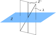
(a)

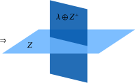
(b)

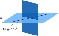
(c)

There is a simple geometric understanding of eq. 3.4. Geometrically the whole problem is to find a 2-plane $\widetilde{\lambda}$ to be orthogonal to the 2-plane $\lambda$ in $\mathbb{C}^{n}$. One way to proceed is to start with a generic 4-plane ${Z}$ and realize that

$$\text{dim}(\lambda^{\perp}\cap Z)=2,$$ (3.7)

where $\lambda^{\perp}$ is the $n-2$ dimensional plane which is orthogonal to $\lambda$. Therefore $\lambda^{\perp}\cap Z$ is a solution of $\widetilde{\lambda}$. It is also easy to find that

$$\lambda^{\perp}\cap Z=(\lambda\oplus Z^{\perp})^{\perp}$$ (3.8)

where $Z^{\perp}$ is the $n-4$ dimensional plane orthogonal to $Z$. One can directly prove that the eq. 3.4 is simply the Plucker coordinate expression of $\widetilde{\lambda}=(\lambda\oplus Z^{\perp})^{\perp}$.

In fact, $\mathcal{S}$ variables can be generalized mathematically, although it might not be physically relevant. The general problem is to find a generic $i$-dimensional plane $\widetilde{\lambda}$ orthogonal to a $j$-dimensional plane $\lambda$. And eq. 3.4 can be generalized as follows

$$(\widetilde{\lambda}_{a_{1}}~{}\widetilde{\lambda}_{a_{2}}~{}\ldots~{}\widetilde{\lambda}_{a_{i}})\sim\sum_{b_{1},b_{2},\ldots,b_{j}=1}^{n}{(\lambda_{b_{1}}~{}\lambda_{b_{2}}~{}\ldots~{}\lambda_{b_{j}})({Z}_{a_{1}}~{}{Z}_{a_{2}}~{}\ldots~{}{Z}_{a_{i}}~{}{Z}_{b_{1}}~{}{Z}_{b_{2}}~{}\ldots~{}{Z}_{b_{j}})},$$ (3.9)

which gives a solution to the problem. Here $Z$ is a generic $(i+j)$-dimensional plane. A brief proof of eq. 3.9 is shown in appendix B.

	Momentum	Spinor	$\begin{array}[]{c}\text{Momentum}\\ \text{Twistor}\end{array}$	$\mathcal{S}$ Variables
$\begin{array}[]{c}\text{Gauge}\\ \text{Degrees of Freedom}\end{array}$	0	$n$	$n+4$	$3n+4$
$\begin{array}[]{c}\text{Total}\\ \text{Degrees of Freedom}\end{array}$	$3n-4$	$4n-4$	$4n$	$6n$
$\begin{array}[]{c}\text{Number of}\\ \text{Constraints}\end{array}$	$n+4$	$4$	$0$	$0$
$\begin{array}[]{c}\text{Massless}\\ \text{Manifest}\end{array}$	No	Yes	Yes	Yes
$\begin{array}[]{c}\text{Momentum Conservation}\\ \text{Manifest}\end{array}$	No	No	Yes	Yes
$\begin{array}[]{c}\text{Permutation}\\ \text{Manifest}\end{array}$	Yes	Yes	No	Yes

Let us now do a simple counting of degrees of freedom to close the section. The physical degrees of freedom of $n$ massless particles is $3n-4$. We could regard a twistor, not in a projective way, but as a 4-component vector with one rescaling gauge degree of freedom. In this way momentum twistors have $n+4$ gauge degrees of freedom, in which the $4$ comes from the fact that a constant translation to each $X_{i}$ does not change the kinematics. Similarly the spinors $\lambda$ and $\widetilde{\lambda}$ also have rescaling gauge. For the $\mathcal{S}$ variables in general(3.9), all $Z$ that satisfy the following form

$$Z=\left(\begin{array}[]{cccccc}1&\cdots&0&0&0&0\\ \vdots&\cdots&\vdots&\vdots&\cdots&\vdots\\ 0&\cdots&1&0&0&0\\ d^{1}_{1}&\cdots&d_{1}^{i}&1&\cdots&0\\ \vdots&\cdots&\vdots&\vdots&\cdots&\vdots\\ d_{j}^{1}&\cdots&d_{j}^{i}&0&\cdots&1\end{array}\right)\left(\begin{array}[]{cccccccc}c_{1}^{1}&c_{1}^{2}&\cdots&\cdots&\cdots&\cdots&c_{1}^{n-1}&c_{1}^{n}\\ \vdots&\vdots&\cdots&\cdots&\cdots&\cdots&\vdots&\vdots\\ c_{i}^{1}&c_{i}^{2}&\cdots&\cdots&\cdots&\cdots&c_{i}^{n-1}&c_{i}^{n}\\ \widetilde{\lambda}_{1}^{1}&\widetilde{\lambda}_{1}^{2}&\cdots&\cdots&\cdots&\cdots&\widetilde{\lambda}_{1}^{n-1}&\widetilde{\lambda}_{1}^{n}\\ \vdots&\vdots&\cdots&\cdots&\cdots&\cdots&\vdots&\vdots\\ \widetilde{\lambda}_{j}^{1}&\widetilde{\lambda}_{j}^{2}&\cdots&\cdots&\cdots&\cdots&\widetilde{\lambda}_{j}^{n-1}&\widetilde{\lambda}_{j}^{n}\end{array}\right)$$ (3.10)

give the same solution $\widetilde{\lambda}$, in which $c$ and $d$ are arbitrary. Therefore the gauge degrees of freedom is rescaling plus all free parameters $c$ and $d$, and their number equals $n+in+ij$. In particular, here when $\lambda$ and $\widetilde{\lambda}$ are 2-component spinors, the number is $3n+4$. We compare all of them including normal 4-component momentum in the table. So we clearly see the “evolution” of variables by introducing more gauge, which makes more physical properties manifest.

4 MHV Amplitudes of Gravity and Soft Factors

As an application of the $\mathcal{S}$ variables, let us consider MHV amplitudes of gravity, which is first obtained in [6]. Here we strip out the momentum conserving delta function and its superpartners. The result for the 4 particles amplitude looks very nice in the $\mathcal{S}$ variables,

$$M_{4}=\left(\prod^{4}_{a<b}\langle a~{}b\rangle\right)^{-1}\langle 1~{}2~{}3~{}4\rangle.$$ (4.1)

The denominator is a product of all non-vanishing angular brackets. As we can see, the result is manifestly permutation invariant. For $n=5$, we get

$$M_{5}=\left(\prod^{5}_{a<b}\langle a~{}b\rangle\right)^{-1}\sum_{s<t,\,i<j<k}^{5}{\langle s~{}t\rangle\langle i~{}j\rangle\langle j~{}k\rangle\langle i~{}k\rangle\overline{\langle s~{}i~{}j~{}k\rangle}\,\overline{\langle t~{}i~{}j~{}k\rangle}},$$ (4.2)

which is again manifestly permutation invariant. The notation $\overline{\langle i~{}j~{}k~{}l\rangle}$ means $i,j,k,l$ are forced to be ordered so that it has the right sign,

$$\overline{\langle i~{}j~{}k~{}l\rangle}=\langle a~{}b~{}c~{}d\rangle,\qquad a,b,c,d\in\{i,j,k,l\},\;\;\;a<b<c<d.$$ (4.3)

For general $n$, we use the recent result[5] of Hodges that

$$M_{n}=(-1)^{n+1}\text{sgn}(\alpha\beta)c_{\alpha(1)\alpha(2)\alpha(3)}c^{\beta(1)\beta(2)\beta(3)}\phi_{[\alpha(4)}^{\beta(4)}\phi_{\alpha(5)}^{\beta(5)}\ldots\phi_{\alpha(n)]}^{\beta(n)}.$$ (4.4)

Here $\phi_{i}^{j}$ is an $n\times n$ matrix. Using our $\mathcal{S}$ variables, $\phi_{i}^{j}$ become the follows

$$\phi_{i}^{j} =\sum_{k,l=1}^{n}{\frac{\langle k~{}l\rangle}{\langle i~{}j\rangle}\langle i~{}j~{}k~{}l\rangle},\qquad i\neq j$$ (4.5)

$$\phi_{i}^{i} =\frac{1}{6}\sum_{j,k,l=1}^{n}{\frac{\langle j~{}k\rangle\langle k~{}l\rangle\langle l~{}j\rangle}{\langle i~{}j\rangle\langle i~{}k\rangle\langle i~{}l\rangle}\langle i~{}j~{}k~{}l\rangle}.$$

In eq. 4.5 the second formula is the soft factor for gravity amplitudes. The permutation invariant property is manifest for all $\phi_{i}^{j}$ and particularly the reference particles disappear in the expression of $\phi_{i}^{i}$. In this sense the $\mathcal{S}$ variables improve the formula for tree level MHV gravity amplitudes in [5].

5 Discussions

A very remarkable property of momentum twistors is that they make the dual conformal symmetry[7] manifest in planar Yang-Mills theory. One of the motivations of this work is the hope that the $\mathcal{S}$ variables will help make properties of gravity manifest. Although there seem to be nothing like dual conformal symmetry, $\mathcal{N}=8$ supergravity is known to have an $E_{7(7)}$ symmetry.

Another hope is that the $\mathcal{S}$ variables could be also useful understanding the KLT[8] and BCJ[9] relations because those relations also depend on the constraints of momentum conservation.

It would also be interesting to find the $\mathcal{S}$ variables form of BCFW[10]. For this purpose it is necessary to understand factorization and we give the first steps in appendix C.

Appendix A Solving Equations

We want to solve eq. 2.3 and find a nice expression of $(\widetilde{\lambda}_{i}~{}\widetilde{\lambda}_{j})$. Here by nice expression, we expect every single factor could be expressed as some kinds of contractions. There are several possible contractions allowed by the little group properties, namely,

$$(\lambda_{i}~{}\lambda_{j}),\quad(\lambda_{i}~{}\eta_{j}),\quad(\lambda_{i}~{}\zeta_{j}),\quad(\zeta_{i}~{}\zeta_{j}),\quad(\eta_{i}~{}\eta_{j}),\quad(\zeta_{i}~{}\eta_{j}),\quad({{Z}}_{i}~{}{{Z}}_{j}~{}{{Z}}_{k}~{}{{Z}}_{l}).$$ (A.1)

Note $({{Z}}_{i}~{}{{Z}}_{j}~{}{{Z}}_{k}~{}{{Z}}_{l})$ is not independent but an antisymmetric sum of products of $(\zeta_{i}~{}\zeta_{j})$ and $(\eta_{i}~{}\eta_{j})$. It is unlikely that all of these contraction will appear inevitably in the expression, so we now try to find a few clues to eliminate a few of them.

We start by writing down the equations in a matrix form. Note that $Y_{ia\dot{a}}$ can actually be independently split into two sets: $Y_{ia1}$ and $Y_{ia2}$. Thus the $4n$ equations can be diagonalized into two sets of independent $2n$ equations with the same array of the coefficients.

$$\left(\begin{array}[]{cccccc}\zeta_{1}^{1}&\zeta_{1}^{2}&0&0&\cdots&\cdots\\ 0&0&\zeta_{2}^{1}&\zeta_{2}^{2}&\cdots&\cdots\\ \vdots&\vdots&\vdots&\vdots&\cdots&\cdots\\ \frac{n-1}{n}\lambda_{1}^{1}&\frac{n-1}{n}\lambda_{1}^{2}&-\frac{1}{n}\lambda_{1}^{1}&-\frac{1}{n}\lambda_{1}^{2}&\cdots&\cdots\\ -\frac{1}{n}\lambda_{2}^{1}&-\frac{1}{n}\lambda_{2}^{2}&\frac{n-1}{n}\lambda_{2}^{1}&\frac{n-1}{n}\lambda_{2}^{2}&\cdots&\cdots\\ \vdots&\vdots&\vdots&\vdots&\cdots&\cdots\end{array}\right)\left(\begin{array}[]{c}Y_{111}\\ Y_{121}\\ Y_{211}\\ Y_{221}\\ \vdots\\ \vdots\end{array}\right)=\left(\begin{array}[]{c}\eta_{11}\\ \eta_{21}\\ \vdots\\ 0\\ 0\\ \vdots\end{array}\right)$$ (A.2)

$$\left(\begin{array}[]{cccccc}\zeta_{1}^{1}&\zeta_{1}^{2}&0&0&\cdots&\cdots\\ 0&0&\zeta_{2}^{1}&\zeta_{2}^{2}&\cdots&\cdots\\ \vdots&\vdots&\vdots&\vdots&\cdots&\cdots\\ \frac{n-1}{n}\lambda_{1}^{1}&\frac{n-1}{n}\lambda_{1}^{2}&-\frac{1}{n}\lambda_{1}^{1}&-\frac{1}{n}\lambda_{1}^{2}&\cdots&\cdots\\ -\frac{1}{n}\lambda_{2}^{1}&-\frac{1}{n}\lambda_{2}^{2}&\frac{n-1}{n}\lambda_{2}^{1}&\frac{n-1}{n}\lambda_{2}^{2}&\cdots&\cdots\\ \vdots&\vdots&\vdots&\vdots&\cdots&\cdots\end{array}\right)\left(\begin{array}[]{c}Y_{112}\\ Y_{122}\\ Y_{212}\\ Y_{222}\\ \vdots\\ \vdots\end{array}\right)=\left(\begin{array}[]{c}\eta_{12}\\ \eta_{22}\\ \vdots\\ 0\\ 0\\ \vdots\end{array}\right)$$ (A.3)

Following Cramer’s formulas, the solutions of $Y_{ia\dot{a}}$ must share the determinant of the coefficient array of the linear equations as a common denominator $D_{n}$. We get

$$D_{n}:=-\frac{1}{n^{n}}\sum_{\sigma\in S_{n}}{(1-n)^{a(\sigma)}\text{sgn}(\sigma)\prod_{i=1}^{n}{(\lambda_{i}~{}\zeta_{\sigma(i)})}}.$$ (A.4)

The numerator is the difficult part. We find it by induction. For the 4 particles case,

$$(\widetilde{\lambda}_{1}~{}\widetilde{\lambda}_{2})=\frac{1}{D_{4}}(\lambda_{3}~{}\lambda_{4})({{Z}}_{1}~{}{{Z}}_{2}~{}{{Z}}_{3}~{}{{Z}}_{4}).$$ (A.5)

Eq. (A.5) gives us some hint of the structure of the numerator. First, from $({{Z}}_{1}~{}{{Z}}_{2}~{}{{Z}}_{3}~{}{{Z}}_{4})$, we can rule out the standalone contraction $(\eta_{i}~{}\eta_{j})$, because we know from eq. A.2 that $(\widetilde{\lambda}_{1}~{}\widetilde{\lambda}_{2})$ must only be degree 2 in $\eta$, which is already in $({{Z}}_{1}~{}{{Z}}_{2}~{}{{Z}}_{3}~{}{{Z}}_{4})$. We also know from eq. A.4 that the denominator has $\lambda$ of degree $n$ and $\zeta$ of degree $n$. Together with eq. 2.4, we conclude that the numerator must have $\lambda$ of degree $n-2$, $\zeta$ of degree $n-2$ and $\eta$ of degree 2.

Now we make a guess based on the above analysis of degrees and eq. A.5. We assume that, for generic $n$, the numerator of $(\widetilde{\lambda}_{i}~{}\widetilde{\lambda}_{j})$ has the contraction $({{Z}}_{a}~{}{{Z}}_{b}~{}{{Z}}_{c}~{}{{Z}}_{d})$ and $(\lambda_{e}~{}\lambda_{f})$, which left with $\lambda$ of degree $n-4$, $\zeta$ of degree $n-4$. It is reasonable to guess that they form a degree $n-4$ polynomial in $(\lambda_{g}~{}\zeta_{h})$. The $n-4$ also coincides with the fact that we do not see this monomial in $n=4$ case. Indeed, for $n=5$, we get

$$(\widetilde{\lambda}_{1}~{}\widetilde{\lambda}_{2})=\frac{1}{D_{5}}[(\lambda_{5}~{}\zeta_{5})(\lambda_{3}~{}\lambda_{4})({{Z}}_{1}~{}{{Z}}_{2}~{}{{Z}}_{3}~{}{{Z}}_{4})\\ +(\lambda_{4}~{}\zeta_{4})(\lambda_{3}~{}\lambda_{5})({{Z}}_{1}~{}{{Z}}_{2}~{}{{Z}}_{3}~{}{{Z}}_{3})+(\lambda_{3}~{}\zeta_{3})(\lambda_{4}~{}\lambda_{5})({{Z}}_{1}~{}{{Z}}_{2}~{}{{Z}}_{4}~{}{{Z}}_{5})]$$ (A.6)

Now it is easy to conjecture the formula to be,

$$(\widetilde{\lambda}_{i}~{}\widetilde{\lambda}_{j})=\frac{1}{D_{n}}\sum_{k,l=1}^{n}{(\lambda_{k}~{}\lambda_{l})({{Z}}_{i}~{}{{Z}}_{j}~{}{{Z}}_{k}~{}{{Z}}_{l})\prod^{n}_{a\neq i,j,k,l}(\lambda_{a}~{}\zeta_{a})}$$ (A.7)

and we have checked numerically that it is correct.

We end the section by discussion of direct gauge fixing for eq. 2.6. Recall our degree counting in section 3, we have the rescaling gauge for each ${Z}_{i}$ and also for $\lambda_{i}$ so we can choose a gauge for $\zeta_{i}$ and $\lambda_{i}$ as follows,

$$\zeta_{i}=\left(\begin{array}[]{c}1\\ \alpha_{i}\end{array}\right),\qquad\lambda_{i}=\left(\begin{array}[]{c}\frac{\beta_{i}}{\alpha_{i}}\\ \beta_{i}+1\end{array}\right)$$ (A.8)

It is clear both $\zeta_{i}$ and $\lambda_{i}$ can run over the projective $\mathbb{CP}^{1}$ independently except several singularities. Under this gauge, each

$$(\lambda_{i}~{}\zeta_{i})=1,\qquad i=1,2,\ldots,n$$ (A.9)

And eq. A.7 literally becomes

$$(\widetilde{\lambda}_{i},\widetilde{\lambda}_{j})=\frac{1}{D_{n}}\sum_{k,l=1}^{n}{(\lambda_{k}~{}\lambda_{l})({{Z}}_{i}~{}{{Z}}_{j}~{}{{Z}}_{k}~{}{{Z}}_{l})}.$$ (A.10)

Appendix B Proof of the Generalized Formula

We split the proof into two steps. First we list a proposition. And we use the proposition to prove the corollary which is eq. 3.9.

Proposition. $V_{i}$ are $k$-component vectors and $W_{i}$ are $(n-k)$-component vectors, $i=1,2,\ldots,n$. $V$ is a $k$-plane and $W$ is a $(n-k)$-plane in $\mathbb{C}^{n}$ that

$$V=(V_{1},V_{2},\ldots,V_{n}),\quad W=(W_{1},W_{2},\ldots,W_{n}),\quad V\perp W.$$ (B.1)

Then $\exists$ constant $\alpha\neq 0$,

$$(V_{a_{1}}~{}V_{a_{2}}~{}\cdots~{}V_{a_{k}})=\frac{\text{sgn}(\sigma)}{\alpha}(W_{\hat{a}_{1}}~{}W_{\hat{a}_{2}}~{}\cdots~{}W_{\hat{a}_{n-k}})$$ (B.2)

for any $a_{1}$, $a_{2}$, …, $a_{k}$ and $\hat{a}_{1}$, $\hat{a}_{2}$, …, $\hat{a}_{n-k}$. Here $\sigma$ is a permutation that

$$\sigma=\left(\begin{array}[]{cccccccc}1&2&\ldots&k&k+1&k+2&\ldots&n\\ a_{1}&a_{2}&\ldots&a_{k}&\hat{a}_{1}&\hat{a}_{2}&\ldots&\hat{a}_{n-k}\end{array}\right).$$ (B.3)

Corollary. $\widetilde{\lambda}_{l}$ are $i$-component vectors, $\lambda_{l}$ are $j$-component vectors and $Z_{l}$ are $(i+j)$-component vectors, $l=1,2,\ldots,n$. $\widetilde{\lambda}$ is a $i$-plane, $\lambda$ is a $j$-plane and $Z$ is a $(i+j)$-plane in $\mathbb{C}^{n}$ that

$$\widetilde{\lambda}=(\widetilde{\lambda}_{1},\widetilde{\lambda}_{2},\ldots,\widetilde{\lambda}_{n}),\quad\lambda=(\lambda_{1},\lambda_{2},\ldots,\lambda_{n}),\quad Z=(Z_{1},Z_{2},\ldots,Z_{n}).$$ (B.4)

If $\widetilde{\lambda}=(\lambda\oplus Z^{\perp})^{\perp}$ then $\exists$ constant $\alpha\neq 0$,

$$(\widetilde{\lambda}_{a_{1}}~{}\widetilde{\lambda}_{a_{2}}~{}\ldots~{}\widetilde{\lambda}_{a_{i}})=\frac{1}{\alpha}\sum_{b_{1},b_{2},\ldots,b_{j}=1}^{n}{(\lambda_{b_{1}}~{}\lambda_{b_{2}}~{}\ldots~{}\lambda_{b_{j}})({Z}_{a_{1}}~{}{Z}_{a_{2}}~{}\ldots~{}{Z}_{a_{i}}~{}{Z}_{b_{1}}~{}{Z}_{b_{2}}~{}\ldots~{}{Z}_{b_{j}})}$$ (B.5)

for any $a_{1}$, $a_{2}$, …, $a_{i}$ and $b_{1}$, $b_{2}$, …, $b_{j}$.

Proof. Let us first define a $k$-plane $X$ and a $(n-i)$-plane $W$ to be

$$X=Z^{\perp},\qquad W=\lambda\oplus Z^{\perp}$$ (B.6)

where $k=n-i-j$. We have the matrix representation of $W$,

$$W=\left(\begin{array}[]{cccccccc}\lambda_{1}^{1}&\lambda_{1}^{2}&\cdots&\cdots&\cdots&\cdots&\lambda_{1}^{n-1}&\lambda_{1}^{n}\\ \vdots&\vdots&\cdots&\cdots&\cdots&\cdots&\vdots&\vdots\\ \lambda_{j}^{1}&\lambda_{j}^{2}&\cdots&\cdots&\cdots&\cdots&\lambda_{j}^{n-1}&\lambda_{j}^{n}\\ X_{1}^{1}&X_{1}^{2}&\cdots&\cdots&\cdots&\cdots&X_{1}^{n-1}&X_{1}^{n}\\ \vdots&\vdots&\cdots&\cdots&\cdots&\cdots&\vdots&\vdots\\ X_{k}^{1}&X_{k}^{2}&\cdots&\cdots&\cdots&\cdots&X_{k}^{n-1}&X_{k}^{n}\end{array}\right).$$ (B.7)

Using the eq. B.2, we have

$$(\widetilde{\lambda}_{a_{1}}~{}\widetilde{\lambda}_{a_{2}}~{}\ldots~{}\widetilde{\lambda}_{a_{i}})=\frac{1}{\alpha_{1}}\text{sgn}(\sigma_{1})(W_{\hat{a}_{1}}~{}W_{\hat{a}_{2}}~{}\cdots~{}W_{\hat{a}_{n-i}}),$$ (B.8)

where $\sigma_{1}$ is a permutation that

$$\sigma_{1}=\left(\begin{array}[]{cccccccc}1&2&\ldots&i&i+1&i+2&\ldots&n\\ a_{1}&a_{2}&\ldots&a_{i}&\hat{a}_{1}&\hat{a}_{2}&\ldots&\hat{a}_{n-i}\end{array}\right).$$ (B.9)

We can see

$$(W_{\hat{a}_{1}}~{}W_{\hat{a}_{2}}~{}\cdots~{}W_{\hat{a}_{n-i}})=\sum_{\sigma\in S_{n-i}}{\text{sgn}(\sigma)(\lambda_{{b_{1}}}~{}\lambda_{{b_{2}}}~{}\ldots~{}\lambda_{{b_{j}}})({X}_{c_{1}}~{}{X}_{c_{2}}~{}\ldots~{}{X}_{c_{k}})},$$ (B.10)

where

$$b_{1}=\sigma(\hat{a}_{1}),\quad b_{2}=\sigma(\hat{a}_{2}),\quad\ldots,\quad b_{j}=\sigma(\hat{a}_{j}),$$ (B.11)

$$c_{1}=\sigma(\hat{a}_{j+1}),\quad c_{2}=\sigma(\hat{a}_{j+2}),\quad\ldots,\quad c_{k}=\sigma(\hat{a}_{n-i}),$$

and $S_{n-i}$ is the set of all permutations of $\{\hat{a}_{1},\hat{a}_{2},\ldots,\hat{a}_{n-i}\}$. Using the eq. B.2 again, we have

$$({X}_{c_{1}}~{}{X}_{c_{2}}~{}\ldots~{}{X}_{c_{k}})=\frac{1}{\alpha_{2}}\text{sgn}(\sigma_{2})({Z}_{a_{1}}~{}{Z}_{a_{2}}~{}\ldots~{}{Z}_{a_{i}}~{}{Z}_{b_{1}}~{}{Z}_{b_{2}}~{}\ldots~{}{Z}_{b_{j}}),$$ (B.12)

$\sigma_{2}$ is a permutation that

$$\sigma_{2}=\left(\begin{array}[]{cccccccccccc}1&2&\ldots&k&k+1&k+2&\ldots&n-j&n-j+1&n-j+2&\ldots&n\\ c_{1}&c_{2}&\ldots&c_{k}&a_{1}&a_{2}&\ldots&a_{i}&b_{1}&b_{2}&\ldots&b_{j}\end{array}\right).$$ (B.13)

With eqs. B.8, B.10 and B.12, we have

$$(\widetilde{\lambda}_{a_{1}}~{}\widetilde{\lambda}_{a_{2}}~{}\ldots~{}\widetilde{\lambda}_{a_{i}})=\frac{1}{\alpha}\sum_{\sigma\in S_{n-i}}{(\lambda_{b_{1}}~{}\lambda_{b_{2}}~{}\ldots~{}\lambda_{b_{j}})({Z}_{a_{1}}~{}{Z}_{a_{2}}~{}\ldots~{}{Z}_{a_{i}}~{}{Z}_{b_{1}}~{}{Z}_{b_{2}}~{}\ldots~{}{Z}_{b_{j}})}.$$ (B.14)

Here we have

$$\frac{1}{\alpha}=(-1)^{(i+j)(n-i-j)}\text{sgn}(\sigma_{1})\frac{1}{\alpha_{1}}\frac{1}{\alpha_{2}},$$ (B.15)

Because determinants are antisymmetric, we can let

$$\sum_{\sigma\in S_{n-i}}\rightarrow\sum_{b_{1},b_{2},\ldots,b_{j}=1}^{n},$$ (B.16)

which finishes the proof.

Appendix C Geometry of Factorization

Factorization arises when the sum of momenta of a subset of particles become massless. We can put an on-shell propagator between the two subsets of particles. Kinematics of the two subsets becomes independent after cutting the propagator. We define the division of the two subsets to be $L$ and $R$ with

$$L\cup R=\{1,2,\ldots,n-1,n\}$$

and two lines $Y_{L}$ and $Y_{R}$ related to the propagator,

$$Y_{L}-\bar{Y} =\sum_{i\in{L}}{(Y_{i}-\bar{Y})}$$

$$Y_{R}-\bar{Y} =\sum_{i\in{R}}{(Y_{i}-\bar{Y})}.$$

Take the 6 particles case as an example. Say $L=\{1,2,3\}$ and $R=\{4,5,6\}$, and we have

$$Y_{L} =Y_{1}+Y_{2}+Y_{3}-2\bar{Y}$$

$$Y_{R} =Y_{4}+Y_{5}+Y_{6}-2\bar{Y}$$

The lines $Y_{L}$ and $Y_{R}$ only intersect with $\bar{Y}$ when factorization arises, as shown in the figure.

And $\{Y_{1},Y_{2},Y_{3},Y_{R}\}$ and $\{Y_{4},Y_{5},Y_{6},Y_{L}\}$ both become momentum conserved by themselves. The center of mass line of both subsets is still $\bar{Y}$.

$$\frac{1}{4}(Y_{R}+Y_{1}+Y_{2}+Y_{3})=\frac{1}{4}(Y_{L}+Y_{4}+Y_{5}+Y_{6})=\bar{Y}$$

References

• [1] Z.ย Xu, D.ย -H.ย Zhang and L.ย Chang, โ€œHelicity Amplitudes for Multiple Bremsstrahlung in Massless Nonabelian Gauge Theories,โ€ Nucl.ย Phys.ย B 291, 392 (1987).
• [2] A.ย Hodges, โ€œEliminating spurious poles from gauge-theoretic amplitudes,โ€ arXiv:0905.1473 [hep-th].
• [3] L.ย F.ย Alday and J.ย M.ย Maldacena, โ€œGluon scattering amplitudes at strong coupling,โ€ JHEP 0706, 064 (2007) [arXiv:0705.0303 [hep-th]].
• [4] N.ย Arkani-Hamed, F.ย Cachazo, C.ย Cheung and J.ย Kaplan, โ€œThe S-Matrix in Twistor Space,โ€ JHEP 1003, 110 (2010) [arXiv:0903.2110 [hep-th]].
• [5] A.ย Hodges, โ€œA simple formula for gravitational MHV amplitudes,โ€ arXiv:1204.1930 [hep-th].
• [6] F.ย A.ย Berends, W.ย T.ย Giele and H.ย Kuijf, โ€œOn relations between multi - gluon and multigraviton scattering,โ€ Phys.ย Lett.ย B 211, 91 (1988).
• [7] J.ย M.ย Drummond, J.ย Henn, G.ย P.ย Korchemsky and E.ย Sokatchev, โ€œDual superconformal symmetry of scattering amplitudes in N=4 super-Yang-Mills theory,โ€ Nucl.ย Phys.ย B 828, 317 (2010) [arXiv:0807.1095 [hep-th]].
• [8] H.ย Kawai, D.ย C.ย Lewellen and S.ย H.ย H.ย Tye, โ€œA Relation Between Tree Amplitudes of Closed and Open Strings,โ€ Nucl.ย Phys.ย B 269, 1 (1986).
• [9] Z.ย Bern, J.ย J.ย M.ย Carrasco and H.ย Johansson, โ€œNew Relations for Gauge-Theory Amplitudes,โ€ Phys.ย Rev.ย D 78, 085011 (2008) [arXiv:0805.3993 [hep-ph]].
• [10] R.ย Britto, F.ย Cachazo, B.ย Feng and E.ย Witten, โ€œDirect proof of tree-level recursion relation in Yang-Mills theory,โ€ Phys.ย Rev.ย Lett.ย  94, 181602 (2005) [hep-th/0501052].