The Viterbo–Maslov Index in Dimension Two

Abstract

We prove a formula that expresses the Viterbo–Maslov index of a smooth strip in an oriented $2$-manifold with boundary curves contained in $1$-dimensional submanifolds in terms the degree function on the complement of the union of the two submanifolds.

1 Introduction

We assume throughout this paper that $\Sigma$ is a connected oriented 2-manifold without boundary and $\alpha,\beta\subset\Sigma$ are connected smooth one dimensional oriented submanifolds without boundary which are closed as subsets of $\Sigma$ and intersect transversally. We do not assume that $\Sigma$ is compact, but when it is, $\alpha$ and $\beta$ are embedded circles. Denote the standard half disc by

$${\mathbb{D}}:=\{z\in{\mathbb{C}}\,|\,{\rm Im}\,z\geq 0,\,|z|\leq 1\}.$$

Let ${\mathcal{D}}$ denote the space of all smooth maps $u:{\mathbb{D}}\to\Sigma$ satisfying the boundary conditions $u({\mathbb{D}}\cap{\mathbb{R}})\subset\alpha$ and $u({\mathbb{D}}\cap S^{1})\subset\beta$. For $x,y\in\alpha\cap\beta$ let ${\mathcal{D}}(x,y)$ denote the subset of all $u\in{\mathcal{D}}$ satisfying the endpoint conditions $u(-1)=x$ and $u(1)=y$. Each $u\in{\mathcal{D}}$ determines a locally constant function ${{\rm w}:\Sigma\setminus(\alpha\cup\beta)\to{\mathbb{Z}}}$ defined as the degree

$${\rm w}(z):=\deg(u,z),\qquad z\in\Sigma\setminus(\alpha\cup\beta).$$

When $z$ is a regular value of $u$ this is the algebraic number of points in the preimage $u^{-1}(z)$. The function ${\rm w}$ depends only on the homotopy class of $u$. We prove that the homotopy class of $u$ is uniquely determined by its endpoints $x,y$ and its degree function ${\rm w}$ (Theorem 2.4). The main theorem of this paper asserts that the Viterbo–Maslov index of an element ${u\in{\mathcal{D}}(x,y)}$ is given by the formula

$$\mu(u)=\frac{m_{x}+m_{y}}{2},$$ (1)

where $m_{x}$ denotes the sum of the four values of ${\rm w}$ encountered when walking along a small circle surrounding $x$, and similarly for $y$ (Theorem 3.4). The formula (1) plays a central role in our combinatorial approach [1, 7] to Floer homology [4, 5]. An appendix contains a proof that the space of paths connecting $\alpha$ to $\beta$ is simply connected under suitable assumptions.

Acknowledgement. We thank David Epstein for explaining to us the proof of Proposition A.1.

2 Chains and Traces

Define a cell complex structure on $\Sigma$ by taking the set of zero-cells to be the set $\alpha\cap\beta$, the set of one-cells to be the set of connected components of $(\alpha\setminus\beta)\cup(\beta\setminus\alpha)$ with compact closure, and the set of two-cells to be the set of connected components of $\Sigma\setminus(\alpha\cup\beta)$ with compact closure. (There is an abuse of language here as the “two-cells” need not be homeomorphs of the open unit disc if the genus of $\Sigma$ is positive and the “one-cells” need not be arcs if $\alpha\cap\beta=\emptyset$.) Define a boundary operator ${\partial}$ as follows. For each two-cell $F$ let ${\partial}F=\sum\pm E,$ where the sum is over the one-cells $E$ which abut $F$ and the plus sign is chosen iff the orientation of $E$ (determined from the given orientations of $\alpha$ and $\beta$) agrees with the boundary orientation of $F$ as a connected open subset of the oriented manifold $\Sigma$. For each one-cell $E$ let ${\partial}E=b-a$ where $a$ and $b$ are the endpoints of the arc $E$ and the orientation of $E$ goes from $a$ to $b$. (The one-cell $E$ is either a subarc of $\alpha$ or a subarc of $\beta$ and both $\alpha$ and $\beta$ are oriented one-manifolds.) For $k=0,1,2$ a $k$-chain is defined to be a formal linear combination (with integer coefficients) of $k$-cells, i.e. a two-chain is a locally constant map $\Sigma\setminus(\alpha\cup\beta)\to{\mathbb{Z}}$ (whose support has compact closure in $\Sigma$) and a one-chain is a locally constant map $(\alpha\setminus\beta)\cup(\beta\setminus\alpha)\to{\mathbb{Z}}$ (whose support has compact closure in $\alpha\cup\beta$). It follows directly from the definitions that ${\partial}^{2}F=0$ for each two-cell $F$.

Each $u\in{\mathcal{D}}$ determines a two-chain ${\rm w}$ via

$${\rm w}(z):=\deg(u,z),\qquad z\in\Sigma\setminus(\alpha\cup\beta).$$ (2)

and a one-chain $\nu$ via

$$\nu(z):=\left\{\begin{array}[]{rl}\deg(u\big{|}_{{\partial}{\mathbb{D}}\cap{\mathbb{R}}\;\,}:{\partial}{\mathbb{D}}\cap{\mathbb{R}}\;\to\alpha,z),&\mbox{for }z\in\alpha\setminus\beta,\\ -\deg(u\big{|}_{{\partial}{\mathbb{D}}\cap S^{1}}:{\partial}{\mathbb{D}}\cap S^{1}\to\beta,z),&\mbox{for }z\in\beta\setminus\alpha.\end{array}\right.$$ (3)

Here we orient the one-manifolds ${\mathbb{D}}\cap{\mathbb{R}}$ and ${\mathbb{D}}\cap S^{1}$ from $-1$ to $+1$. For any one-chain $\nu:(\alpha\setminus\beta)\cup(\beta\setminus\alpha)\to{\mathbb{Z}}$ denote

$$\nu_{\alpha}:=\nu|_{\alpha\setminus\beta}:\alpha\setminus\beta\to{\mathbb{Z}},\qquad\nu_{\beta}:=\nu|_{\alpha\setminus\beta}:\beta\setminus\alpha\to{\mathbb{Z}}.$$

Conversely, given locally constant functions $\nu_{\alpha}:\alpha\setminus\beta\to{\mathbb{Z}}$ and $\nu_{\beta}:\beta\setminus\alpha\to{\mathbb{Z}}$, denote by $\nu=\nu_{\alpha}-\nu_{\beta}$ the one-chain that agrees with $\nu_{\alpha}$ on $\alpha\setminus\beta$ and agrees with $-\nu_{\beta}$ on $\beta\setminus\alpha$.

Definition 2.1 (Traces).

Fix two (not necessarily distinct) intersection points $x,y\in\alpha\cap\beta$.

(i) Let ${\rm w}:\Sigma\setminus(\alpha\cup\beta)\to{\mathbb{Z}}$ be a two-chain. The triple $\Lambda=(x,y,{\rm w})$ is called an $(\alpha,\beta)$-trace if there exists an element $u\in{\mathcal{D}}(x,y)$ such that ${\rm w}$ is given by (2). In this case $\Lambda=:\Lambda_{u}$ is also called the $(\alpha,\beta)$-trace of $u$ and we sometimes write ${\rm w}_{u}:={\rm w}$.

(ii) Let $\Lambda=(x,y,{\rm w})$ be an $(\alpha,\beta)$-trace. The triple ${\partial}\Lambda:=(x,y,{\partial}{\rm w})$ is called the boundary of $\Lambda$.

(iii) A one-chain $\nu:(\alpha\setminus\beta)\cup(\beta\setminus\alpha)\to{\mathbb{Z}}$ is called an $(x,y)$-trace if there exist smooth curves $\gamma_{\alpha}:[0,1]\to\alpha$ and $\gamma_{\beta}:[0,1]\to\beta$ such that $\gamma_{\alpha}(0)=\gamma_{\beta}(0)=x$, $\gamma_{\alpha}(1)=\gamma_{\beta}(1)=y$, $\gamma_{\alpha}$ and $\gamma_{\beta}$ are homotopic in $\Sigma$ with fixed endpoints, and

$$\nu(z)=\left\{\begin{array}[]{rl}\deg(\gamma_{\alpha},z),&\mbox{for }z\in\alpha\setminus\beta,\\ -\deg(\gamma_{\beta},z),&\mbox{for }z\in\beta\setminus\alpha.\end{array}\right.$$ (4)

Remark 2.2.

Assume $\Sigma$ is simply connected. Then the condition on $\gamma_{\alpha}$ and $\gamma_{\beta}$ to be homotopic with fixed endpoints is redundant. Moreover, if $x=y$ then a one-chain $\nu$ is an $(x,y)$-trace if and only if the restrictions $\nu_{\alpha}:=\nu|_{\alpha\setminus\beta}$ and $\nu_{\beta}:=-\nu|_{\beta\setminus\alpha}$ are constant. If $x\neq y$ and $\alpha,\beta$ are embedded circles and $A,B$ denote the positively oriented arcs from $x$ to $y$ in $\alpha,\beta$, then a one-chain $\nu$ is an $(x,y)$-trace if and only if $\nu_{\alpha}|_{\alpha\setminus(A\cup\beta)}=\nu_{\alpha}|_{A\setminus\beta}-1$ and $\nu_{\beta}|_{\beta\setminus(B\cup\alpha)}=\nu_{\beta}|_{B\setminus\alpha}-1.$ In particular, when walking along $\alpha$ or $\beta$, the function $\nu$ only changes its value at $x$ and $y$.

Lemma 2.3.

Let $x,y\in\alpha\cap\beta$ and $u\in{\mathcal{D}}(x,y)$. Then the boundary of the $(\alpha,\beta)$-trace $\Lambda_{u}$ of $u$ is the triple ${\partial}\Lambda_{u}=(x,y,\nu),$ where $\nu$ is given by (3). In other words, if ${\rm w}$ is given by (2) and $\nu$ is given by (3) then $\nu={\partial}{\rm w}$.

Proof.

Choose an embedding $\gamma:[-1,1]\to\Sigma$ such that $u$ is transverse to $\gamma$, $\gamma(t)\in\Sigma\setminus(\alpha\cup\beta)$ for $t\neq 0$, $\gamma(-1)$, $\gamma(1)$ are regular values of $u$, ${\gamma(0)\in\alpha\setminus\beta}$ is a regular value of $u|_{{\mathbb{D}}\cap{\mathbb{R}}}$, and $\gamma$ intersects $\alpha$ transversally at $t=0$ such that orientations match in

$$T_{\gamma(0)}\Sigma=T_{\gamma(0)}\alpha\oplus{\mathbb{R}}\dot{\gamma}(0).$$

Denote $\Gamma:=\gamma([-1,1])$. Then $u^{-1}(\Gamma)\subset{\mathbb{D}}$ is a $1$-dimensional submanifold with boundary

$${\partial}u^{-1}(\Gamma)=u^{-1}(\gamma(-1))\cup u^{-1}(\gamma(1))\cup\bigl{(}u^{-1}(\gamma(0))\cap{\mathbb{R}})\bigr{)}.$$

If $z\in u^{-1}(\Gamma)$ then

$${\rm im}\,du(z)+T_{u(z)}\Gamma=T_{u(z)}\Sigma,\qquad T_{z}u^{-1}(\Gamma)=du(z)^{-1}T_{u(z)}\Gamma.$$

We orient $u^{-1}(\Gamma)$ such that the orientations match in

$$T_{u(z)}\Sigma=T_{u(z)}\Gamma\oplus du(z){\mathbf{i}}T_{z}u^{-1}(\Gamma).$$

In other words, if $z\in u^{-1}(\Gamma)$ and $u(z)=\gamma(t)$, then a nonzero tangent vector $\zeta\in T_{z}u^{-1}(\Gamma)$ is positive if and only if the pair $(\dot{\gamma}(t),du(z){\mathbf{i}}\zeta)$ is a positive basis of $T_{\gamma(t)}\Sigma$. Then the boundary orientation of $u^{-1}(\Gamma)$ at the elements of $u^{-1}(\gamma(1))$ agrees with the algebraic count in the definition of ${\rm w}(\gamma(1))$, at the elements of $u^{-1}(\gamma(-1))$ is opposite to the algebraic count in the definition of ${\rm w}(\gamma(-1))$, and at the elements of $u^{-1}(\gamma(0))\cap{\mathbb{R}}$ is opposite to the algebraic count in the definition of $\nu(\gamma(0))$. Hence

$${\rm w}(\gamma(1))={\rm w}(\gamma(-1))+\nu(\gamma(0)).$$

In other words the value of $\nu$ at a point in $\alpha\setminus\beta$ is equal to the value of ${\rm w}$ slightly to the left of $\alpha$ minus the value of ${\rm w}$ slightly to the right of $\alpha$. Likewise, the value of $\nu$ at a point in $\beta\setminus\alpha$ is equal to the value of ${\rm w}$ slightly to the right of $\beta$ minus the value of ${\rm w}$ slightly to the left of $\beta$. This proves Lemma 2.3. ∎

Theorem 2.4.

(i) Two elements of ${\mathcal{D}}$ belong to the same connected component of ${\mathcal{D}}$ if and only if they have the same $(\alpha,\beta)$-trace.

(ii) Assume $\Sigma$ is diffeomorphic to the two-sphere. Then $\Lambda=(x,y,{\rm w})$ is an $(\alpha,\beta)$-trace if and only if ${\partial}{\rm w}$ is an $(x,y)$-trace.

(iii) Assume $\Sigma$ is not diffeomorphic to the two-sphere and let $x,y\in\alpha\cap\beta$. If $\nu$ is an $(x,y)$-trace, then there is a unique two-chain ${\rm w}$ such that $\Lambda:=(x,y,{\rm w})$ is an $(\alpha,\beta)$-trace and ${\partial}{\rm w}=\nu$.

Proof.

We prove (i). “Only if” follows from the standard arguments in degree theory as in Milnor [6]. To prove “if”, fix two intersection points

$$x,y\in\alpha\cap\beta$$

and, for $X=\Sigma,\alpha,\beta$, denote by ${\mathcal{P}}(x,y;X)$ the space of all smooth curves ${\gamma:[0,1]\to X}$ satisfying $\gamma(0)=x$ and $\gamma(1)=y$. Every $u\in{\mathcal{D}}(x,y)$ determines smooth paths $\gamma_{u,\alpha}\in{\mathcal{P}}(x,y;\alpha)$ and $\gamma_{u,\beta}\in{\mathcal{P}}(x,y;\beta)$ via

$$\gamma_{u,\alpha}(s):=u(-\cos(\pi s),0),\qquad\gamma_{u,\beta}(s)=u(-\cos(\pi s),\sin(\pi s)).$$ (5)

These paths are homotopic in $\Sigma$ with fixed endpoints. An explicit homotopy is the map

$$F_{u}:=u\circ{\varphi}:[0,1]^{2}\to\Sigma$$

where ${\varphi}:[0,1]^{2}\to{\mathbb{D}}$ is the map

$${\varphi}(s,t):=(-\cos(\pi s),t\sin(\pi s)).$$

By Lemma 2.3, he homotopy class of $\gamma_{u,\alpha}$ in ${\mathcal{P}}(x,y;\alpha)$ is uniquely determined by $\nu_{\alpha}:={\partial}{\rm w}_{u}|_{\alpha\setminus\beta}:\alpha\setminus\beta\to{\mathbb{Z}}$ and that of $\gamma_{u,\beta}$ in ${\mathcal{P}}(x,y;\beta)$ is uniquely determined by $\nu_{\beta}:=-{\partial}{\rm w}_{u}|_{\beta\setminus\alpha}:\beta\setminus\alpha\to{\mathbb{Z}}$. Hence they are both uniquely determined by the $(\alpha,\beta)$-trace of $u$. If $\Sigma$ is not diffeomorphic to the $2$-sphere the assertion follows from the fact that each component of ${\mathcal{P}}(x,y;\Sigma)$ is contractible (because the universal cover of $\Sigma$ is diffeomorphic to the complex plane). Now assume $\Sigma$ is diffeomorphic to the $2$-sphere. Then $\pi_{1}({\mathcal{P}}(x,y;\Sigma))={\mathbb{Z}}$ acts on $\pi_{0}({\mathcal{D}})$ because the correspondence $u\mapsto F_{u}$ identifies $\pi_{0}({\mathcal{D}})$ with a space of homotopy classes of paths in ${\mathcal{P}}(x,y;\Sigma)$ connecting ${\mathcal{P}}(x,y;\alpha)$ to ${\mathcal{P}}(x,y;\beta)$. The induced action on the space of two-chains ${\rm w}:\Sigma\setminus(\alpha\cup\beta)$ is given by adding a global constant. Hence the map $u\mapsto{\rm w}$ induces an injective map

$$\pi_{0}({\mathcal{D}}(x,y))\to\{\mbox{$2$-chains}\}.$$

This proves (i).

We prove (ii) and (iii). Let ${\rm w}$ be a two-chain, suppose that

$$\nu:={\partial}{\rm w}$$

is an $(x,y)$-trace, and denote

$$\Lambda:=(x,y,{\rm w}).$$

Let ${\gamma_{\alpha}:[0,1]\to\alpha}$ and ${\gamma_{\beta}:[0,1]\to\beta}$ be as in Definition 2.1. Then there is a $u^{\prime}\in{\mathcal{D}}(x,y)$ such that the map $s\mapsto u^{\prime}(-\cos(\pi s),0)$ is homotopic to $\gamma_{\alpha}$ and $s\mapsto u^{\prime}(-\cos(\pi s),\sin(\pi s))$ is homotopic to $\gamma_{\beta}$. By definition the $(\alpha,\beta)$-trace of $u^{\prime}$ is $\Lambda^{\prime}=(x,y,{\rm w}^{\prime})$ for some two-chain ${\rm w}^{\prime}$. By Lemma 2.3, we have

$${\partial}{\rm w}^{\prime}=\nu={\partial}{\rm w}$$

and hence ${\rm w}-{\rm w}^{\prime}=:d$ is constant. If $\Sigma$ is not diffeomorphic to the two-sphere and $\Lambda$ is the $(\alpha,\beta)$-trace of some element $u\in{\mathcal{D}}$, then $u$ is homotopic to $u^{\prime}$ (as ${\mathcal{P}}(x,y;\Sigma)$ is simply connected) and hence $d=0$ and $\Lambda=\Lambda^{\prime}$. If $\Sigma$ is diffeomorphic to the $2$-sphere choose a smooth map $v:S^{2}\to\Sigma$ of degree $d$ and replace $u^{\prime}$ by the connected sum $u:=u^{\prime}\#v$. Then $\Lambda$ is the $(\alpha,\beta)$-trace of $u$. This proves Theorem 2.4. ∎

Remark 2.5.

Let $\Lambda=(x,y,{\rm w})$ be an $(\alpha,\beta)$-trace and define

$$\nu_{\alpha}:={\partial}{\rm w}|_{\alpha\setminus\beta},\qquad\nu_{\beta}:=-{\partial}{\rm w}|_{\beta\setminus\alpha}.$$

(i) The two-chain ${\rm w}$ is uniquely determined by the condition ${\partial}{\rm w}=\nu_{\alpha}-\nu_{\beta}$ and its value at one point. To see this, think of the embedded circles $\alpha$ and $\beta$ as traintracks. Crossing $\alpha$ at a point $z\in\alpha\setminus\beta$ increases ${\rm w}$ by $\nu_{\alpha}(z)$ if the train comes from the left, and decreases it by $\nu_{\alpha}(z)$ if the train comes from the right. Crossing $\beta$ at a point $z\in\beta\setminus\alpha$ decreases ${\rm w}$ by $\nu_{\beta}(z)$ if the train comes from the left and increases it by $\nu_{\beta}(z)$ if the train comes from the right. Moreover, $\nu_{\alpha}$ extends continuously to $\alpha\setminus\{x,y\}$ and $\nu_{\beta}$ extends continuously to $\beta\setminus\{x,y\}$. At each intersection point $z\in(\alpha\cap\beta)\setminus\{x,y\}$ with intersection index $+1$ (respectively $-1$) the function ${\rm w}$ takes the values

$$k,\quad k+\nu_{\alpha}(z),\quad k+\nu_{\alpha}(z)-\nu_{\beta}(z),\quad k-\nu_{\beta}(z)$$

as we march counterclockwise (respectively clockwise) along a small circle surrounding the intersection point.

(ii) If $\Sigma$ is not diffeomorphic to the $2$-sphere then, by Theorem 2.4 (iii), the $(\alpha,\beta)$-trace $\Lambda$ is uniquely determined by its boundary ${\partial}\Lambda=(x,y,\nu_{\alpha}-\nu_{\beta})$.

(iii) Assume $\Sigma$ is not diffeomorphic to the $2$-sphere and choose a universal covering $\pi:{\mathbb{C}}\to\Sigma$. Choose a point ${\tilde{x}}\in\pi^{-1}(x)$ and lifts ${\tilde{\alpha}}$ and ${\tilde{\beta}}$ of $\alpha$ and $\beta$ such that ${\tilde{x}}\in{\tilde{\alpha}}\cap{\tilde{\beta}}.$ Then $\Lambda$ lifts to an $({\tilde{\alpha}},{\tilde{\beta}})$-trace

$${\tilde{\Lambda}}=({\tilde{x}},{\tilde{y}},\tilde{\rm w}).$$

More precisely, the one chain $\nu:=\nu_{\alpha}-\nu_{\beta}={\partial}{\rm w}$ is an $(x,y)$-trace, by Lemma 2.3. The paths $\gamma_{\alpha}:[0,1]\to\alpha$ and $\gamma_{\beta}:[0,1]\to\beta$ in Definition 2.1 lift to unique paths $\gamma_{\tilde{\alpha}}:[0,1]\to{\tilde{\alpha}}$ and $\gamma_{\tilde{\beta}}:[0,1]\to{\tilde{\beta}}$ connecting ${\tilde{x}}$ to ${\tilde{y}}$. For ${\tilde{z}}\in{\mathbb{C}}\setminus({\tilde{A}}\cup{\tilde{B}})$ the number $\tilde{\rm w}({\tilde{z}})$ is the winding number of the loop $\gamma_{\tilde{\alpha}}-\gamma_{\tilde{\beta}}$ about ${\tilde{z}}$ (by Rouché’s theorem). The two-chain ${\rm w}$ is then given by

$${\rm w}(z)=\sum_{{\tilde{z}}\in\pi^{-1}(z)}\tilde{\rm w}({\tilde{z}}),\qquad z\in\Sigma\setminus(\alpha\cup\beta).$$

To see this, lift an element $u\in{\mathcal{D}}(x,y)$ with $(\alpha,\beta)$-trace $\Lambda$ to the universal cover to obtain an element ${\tilde{u}}\in{\mathcal{D}}({\tilde{x}},{\tilde{y}})$ with $\Lambda_{\tilde{u}}={\tilde{\Lambda}}$ and consider the degree.

Definition 2.6 (Catenation).

Let $x,y,z\in\alpha\cap\beta$. The catenation of two $(\alpha,\beta)$-traces $\Lambda=(x,y,{\rm w})$ and $\Lambda^{\prime}=(y,z,{\rm w}^{\prime})$ is defined by

$$\Lambda\#\Lambda^{\prime}:=(x,z,{\rm w}+{\rm w}^{\prime}).$$

Let $u\in{\mathcal{D}}(x,y)$ and $u^{\prime}\in{\mathcal{D}}(y,z)$ and suppose that $u$ and $u^{\prime}$ are constant near the ends $\pm 1\in{\mathbb{D}}$. For $0<\lambda<1$ sufficiently close to one the $\lambda$-catenation of $u$ and $u^{\prime}$ is the map $u\#_{\lambda}u^{\prime}\in{\mathcal{D}}(x,z)$ defined by

$$(u\#_{\lambda}u^{\prime})(\zeta):=\left\{\begin{array}[]{ll}u\left(\frac{\zeta+\lambda}{1+\lambda\zeta}\right),&\mbox{for }{\rm Re}\,\zeta\leq 0,\\ u^{\prime}\left(\frac{\zeta-\lambda}{1-\lambda\zeta}\right),&\mbox{for }{\rm Re}\,\zeta\geq 0.\end{array}\right.$$

Lemma 2.7.

If $u\in{\mathcal{D}}(x,y)$ and $u^{\prime}\in{\mathcal{D}}(y,z)$ are as in Definition 2.6 then

$$\Lambda_{u\#_{\lambda}u^{\prime}}=\Lambda_{u}\#\Lambda_{u^{\prime}}.$$

Thus the catenation of two $(\alpha,\beta)$-traces is again an $(\alpha,\beta)$-trace.

Proof.

This follows directly from the definitions. ∎

3 The Maslov Index

Definition 3.1.

Let $x,y\in\alpha\cap\beta$ and $u\in{\mathcal{D}}(x,y)$. Choose an orientation preserving trivialization

$${\mathbb{D}}\times{\mathbb{R}}^{2}\to u^{*}T\Sigma:(z,\zeta)\mapsto\Phi(z)\zeta$$

and consider the Lagrangian paths

$$\lambda_{0},\lambda_{1}:[0,1]\to{\mathbb{R}\mathrm{P}}^{1}$$

given by

$$\begin{split}\lambda_{0}(s)&:=\Phi(-\cos(\pi s),0)^{-1}T_{u(-\cos(\pi s),0)}\alpha,\\ \lambda_{1}(s)&:=\Phi(-\cos(\pi s),\sin(\pi s))^{-1}T_{u(-\cos(\pi s),\sin(\pi s))}\beta.\end{split}$$

The Viterbo–Maslov index of $u$ is defined as the relative Maslov index of the pair of Lagrangian paths $(\lambda_{0},\lambda_{1})$ and will be denoted by

$$\mu(u):=\mu(\Lambda_{u}):=\mu(\lambda_{0},\lambda_{1}).$$

By the naturality and homotopy axioms for the relative Maslov index (see for example [8]), the number $\mu(u)$ is independent of the choice of the trivialization and depends only on the homotopy class of $u$; hence it depends only on the $(\alpha,\beta)$-trace of $u$, by Theorem 2.4. The relative Maslov index $\mu(\lambda_{0},\lambda_{1})$ is the degree of the loop in ${\mathbb{R}\mathrm{P}}^{1}$ obtained by traversing $\lambda_{0}$, followed by a counterclockwise turn from $\lambda_{0}(1)$ to $\lambda_{1}(1)$, followed by traversing $\lambda_{1}$ in reverse time, followed by a clockwise turn from $\lambda_{1}(0)$ to $\lambda_{0}(0)$. This index was first defined by Viterbo [9] (in all dimensions). Another exposition is contained in [8].

Remark 3.2.

The Viterbo–Maslov index is additive under catenation, i.e. if

$$\Lambda=(x,y,{\rm w}),\qquad\Lambda^{\prime}=(y,z,{\rm w}^{\prime})$$

are $(\alpha,\beta)$-traces then

$$\mu(\Lambda\#\Lambda^{\prime})=\mu(\Lambda)+\mu(\Lambda^{\prime}).$$

For a proof of this formula see [9, 8].

Definition 3.3.

Let $\Lambda=(x,y,{\rm w})$ be an $(\alpha,\beta)$-trace and

$$\nu_{\alpha}:={\partial}{\rm w}|_{\alpha\setminus\beta},\qquad\nu_{\beta}:=-{\partial}{\rm w}|_{\beta\setminus\alpha}.$$

$\Lambda$ is said to satisfy the arc condition if

$$x\neq y,\qquad\min\left|\nu_{\alpha}\right|=\min\left|\nu_{\beta}\right|=0.$$ (6)

When $\Lambda$ satisfies the arc condition there are arcs $A\subset\alpha$ and $B\subset\beta$ from $x$ to $y$ such that

$$\nu_{\alpha}(z)=\left\{\begin{array}[]{rl}\pm 1,&\mbox{if }z\in A,\\ 0,&\mbox{if }z\in\alpha\setminus\overline{A},\end{array}\right.\;\;\nu_{\beta}(z)=\left\{\begin{array}[]{rl}\pm 1,&\mbox{if }z\in B,\\ 0,&\mbox{if }z\in\beta\setminus\overline{B}.\end{array}\right.$$ (7)

Here the plus sign is chosen iff the orientation of $A$ from $x$ to $y$ agrees with that of $\alpha$, respectively the orientation of $B$ from $x$ to $y$ agrees with that of $\beta$. In this situation the quadruple $(x,y,A,B)$ and the triple $(x,y,{\partial}{\rm w})$ determine one another and we also write

$${\partial}\Lambda=(x,y,A,B)$$

for the boundary of $\Lambda$. When $u\in{\mathcal{D}}$ and $\Lambda_{u}=(x,y,{\rm w})$ satisfies the arc condition and ${\partial}\Lambda_{u}=(x,y,A,B)$ then

$$s\mapsto u(-\cos(\pi s),0)$$

is homotopic in $\alpha$ to a path traversing $A$ and the path

$$s\mapsto u(-\cos(\pi s),\sin(\pi s))$$

is homotopic in $\beta$ to a path traversing $B$.

Theorem 3.4.

Let $\Lambda=(x,y,{\rm w})$ be an $(\alpha,\beta)$-trace. For $z\in\alpha\cap\beta$ denote by $m_{z}(\Lambda)$ the sum of the four values of ${\rm w}$ encountered when walking along a small circle surrounding $z$. Then the Viterbo–Maslov index of $\Lambda$ is given by

$$\mu(\Lambda)=\frac{m_{x}(\Lambda)+m_{y}(\Lambda)}{2}.$$ (8)

We first prove the result for the $2$-plane and the $2$-sphere (Section 4). When $\Sigma$ is not simply connected we reduce the result to the case of the $2$-plane (Section 5). The key is the identity

$$m_{g{\tilde{x}}}({\tilde{\Lambda}})+m_{g^{-1}{\tilde{y}}}({\tilde{\Lambda}})=0$$ (9)

for every lift ${\tilde{\Lambda}}$ to the universal cover and every deck transformation $g\neq{\rm id}$.

4 The Simply Connected Case

A connected oriented $2$-manifold $\Sigma$ is called planar if it admits an (orientation preserving) embedding into the complex plane.

Proposition 4.1.

Equation (8) holds when $\Sigma$ is planar.

Proof.

Assume first that $\Sigma={\mathbb{C}}$ and $\Lambda=(x,y,{\rm w})$ satisfies the arc condition. Thus the boundary of $\Lambda$ has the form

$${\partial}\Lambda=(x,y,A,B),$$

where $A\subset\alpha$ and $B\subset\beta$ are arcs from $x$ to $y$ and ${\rm w}(z)$ is the winding number of the loop $A-B$ about the point $z\in\Sigma\setminus(A\cup B)$ (see Remark 2.5). Hence the formula (8) can be written in the form

$$\mu(\Lambda)=2k_{x}+2k_{y}+\frac{{\varepsilon}_{x}-{\varepsilon}_{y}}{2}.$$ (10)

Here ${\varepsilon}_{z}={\varepsilon}_{z}(\Lambda)\in\{+1,-1\}$ denotes the intersection index of $A$ and $B$ at a point $z\in A\cap B$, $k_{x}=k_{x}(\Lambda)$ denotes the value of the winding number ${\rm w}$ at a point in $\alpha\setminus A$ close to $x$, and $k_{y}=k_{y}(\Lambda)$ denotes the value of ${\rm w}$ at a point in $\alpha\setminus A$ close to $y$. We now prove (10) under the assumption that $\Lambda$ satisfies the arc condition. The proof is by induction on the number of intersection points of $B$ and $\alpha$ and has seven steps.

Step 1. We may assume without loss of generality that

$$\Sigma={\mathbb{C}},\qquad\alpha={\mathbb{R}},\qquad A=[x,y],\qquad x<y,$$ (11)

and $B\subset{\mathbb{C}}$ is an embedded arc from $x$ to $y$ that is transverse to ${\mathbb{R}}$.

Choose a diffeomorphism from $\Sigma$ to ${\mathbb{C}}$ that maps $A$ to a bounded closed interval and maps $x$ to the left endpoint of $A$. If $\alpha$ is not compact the diffeomorphism can be chosen such that it also maps $\alpha$ to ${\mathbb{R}}$. If $\alpha$ is an embedded circle the diffeomorphism can be chosen such that its restriction to $B$ is transverse to ${\mathbb{R}}$; now replace the image of $\alpha$ by ${\mathbb{R}}$. This proves Step 1.

Step 2. Assume (11) and let $\bar{\Lambda}:=(x,y,z\mapsto-{\rm w}(\bar{z}))$ be the $(\alpha,\bar{\beta})$-trace obtained from $\Lambda$ by complex conjugation. Then $\Lambda$ satisfies (10) if and only if $\bar{\Lambda}$ satisfies (10).

Step 2 follows from the fact that the numbers $\mu,k_{x},k_{y},{\varepsilon}_{x},{\varepsilon}_{y}$ change sign under complex conjugation.

Step 3. Assume (11). If $B\cap{\mathbb{R}}=\{x,y\}$ then $\Lambda$ satisfies (10).

In this case $B$ is contained in the upper or lower closed half plane and the loop $A\cup B$ bounds a disc contained in the same half plane. By Step 1 we may assume that $B$ is contained in the upper half space. Then ${\varepsilon}_{x}=1$, ${\varepsilon}_{y}=-1$, and $\mu(\Lambda)=1$. Moreover, the winding number ${\rm w}$ is one in the disc encircled by $A$ and $B$ and is zero in the complement of its closure. Since the intervals $(-\infty,0)$ and $(0,\infty)$ are contained in this complement, we have $k_{x}=k_{y}=0$. This proves Step 3.

Step 4. Assume (11) and $\#(B\cap{\mathbb{R}})>2$, follow the arc of $B$, starting at $x$, and let $x^{\prime}$ be the next intersection point with ${\mathbb{R}}$. Assume $x^{\prime}<x$, denote by $B^{\prime}$ the arc in $B$ from $x^{\prime}$ to $y$, and let $A^{\prime}:=[x^{\prime},y]$ (see Figure 1). If the $(\alpha,\beta)$-trace $\Lambda^{\prime}$ with boundary ${\partial}\Lambda^{\prime}=(x^{\prime},y,A^{\prime},B^{\prime})$ satisfies (10) so does $\Lambda$.

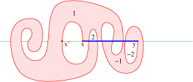
Figure 1: Maslov index and catenation: $x^{\prime}<x<y$.

By Step 2 we may assume ${\varepsilon}_{x}(\Lambda)=1$. Orient $B$ from $x$ to $y$. The Viterbo–Maslov index of $\Lambda$ is minus the Maslov index of the path $B\to{\mathbb{R}\mathrm{P}}^{1}:z\mapsto T_{z}B,$ relative to the Lagrangian subspace ${\mathbb{R}}\subset{\mathbb{C}}$. Since the Maslov index of the arc in $B$ from $x$ to $x^{\prime}$ is $+1$ we have

$$\mu(\Lambda)=\mu(\Lambda^{\prime})-1.$$ (12)

Since the orientations of $A^{\prime}$ and $B^{\prime}$ agree with those of $A$ and $B$ we have

$${\varepsilon}_{x^{\prime}}(\Lambda^{\prime})={\varepsilon}_{x^{\prime}}(\Lambda)=-1,\qquad{\varepsilon}_{y}(\Lambda^{\prime})={\varepsilon}_{y}(\Lambda).$$ (13)

Now let $x_{1}<x_{2}<\cdots<x_{m}<x$ be the intersection points of ${\mathbb{R}}$ and $B$ in the interval $(-\infty,x)$ and let ${\varepsilon}_{i}\in\{-1,+1\}$ be the intersection index of ${\mathbb{R}}$ and $B$ at $x_{i}$. Then there is an integer $\ell\in\{1,\dots,m\}$ such that $x_{\ell}=x^{\prime}$ and ${\varepsilon}_{\ell}=-1$. Moreover, the winding number ${\rm w}$ slightly to the left of $x$ is

$$k_{x}(\Lambda)=\sum_{i=1}^{m}{\varepsilon}_{i}.$$

It agrees with the value of ${\rm w}$ slightly to the right of $x^{\prime}=x_{\ell}$. Hence

$$k_{x}(\Lambda)=\sum_{i=1}^{\ell}{\varepsilon}_{i}=\sum_{i=1}^{\ell-1}{\varepsilon}_{i}-1=k_{x^{\prime}}(\Lambda^{\prime})-1,\qquad k_{y}(\Lambda^{\prime})=k_{y}(\Lambda).$$ (14)

It follows from equation (10) for $\Lambda^{\prime}$ and equations (12), (13), and (14) that

$$\mu(\Lambda) = \mu(\Lambda^{\prime})-1$$

$$= 2k_{x^{\prime}}(\Lambda^{\prime})+2k_{y}(\Lambda^{\prime})+\frac{{\varepsilon}_{x^{\prime}}(\Lambda^{\prime})-{\varepsilon}_{y}(\Lambda^{\prime})}{2}-1$$

$$= 2k_{x^{\prime}}(\Lambda^{\prime})+2k_{y}(\Lambda^{\prime})+\frac{-1-{\varepsilon}_{y}(\Lambda)}{2}-1$$

$$= 2k_{x^{\prime}}(\Lambda^{\prime})+2k_{y}(\Lambda^{\prime})+\frac{1-{\varepsilon}_{y}(\Lambda)}{2}-2$$

$$= 2k_{x}(\Lambda)+2k_{y}(\Lambda)+\frac{{\varepsilon}_{x}(\Lambda)-{\varepsilon}_{y}(\Lambda)}{2}.$$

This proves Step 4.

Step 5. Assume (11) and $\#(B\cap{\mathbb{R}})>2$, follow the arc of $B$, starting at $x$, and let $x^{\prime}$ be the next intersection point with ${\mathbb{R}}$. Assume $x<x^{\prime}<y$, denote by $B^{\prime}$ the arc in $B$ from $x^{\prime}$ to $y$, and let $A^{\prime}:=[x^{\prime},y]$ (see Figure 2). If the $(\alpha,\beta)$-trace $\Lambda^{\prime}$ with boundary ${\partial}\Lambda^{\prime}=(x^{\prime},y,A^{\prime},B^{\prime})$ satisfies (10) so does $\Lambda$.

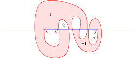
Figure 2: Maslov index and catenation: $x<x^{\prime}<y$.

By Step 2 we may assume ${\varepsilon}_{x}(\Lambda)=1$. Since the Maslov index of the arc in $B$ from $x$ to $x^{\prime}$ is $-1$, we have

$$\mu(\Lambda)=\mu(\Lambda^{\prime})+1.$$ (15)

Since the orientations of $A^{\prime}$ and $B^{\prime}$ agree with those of $A$ and $B$ we have

$${\varepsilon}_{x^{\prime}}(\Lambda^{\prime})={\varepsilon}_{x^{\prime}}(\Lambda)=-1,\qquad{\varepsilon}_{y}(\Lambda^{\prime})={\varepsilon}_{y}(\Lambda).$$ (16)

Now let $x<x_{1}<x_{2}<\cdots<x_{m}<x^{\prime}$ be the intersection points of ${\mathbb{R}}$ and $B$ in the interval $(x,x^{\prime})$ and let ${\varepsilon}_{i}\in\{-1,+1\}$ be the intersection index of ${\mathbb{R}}$ and $B$ at $x_{i}$. Since the value of ${\rm w}$ slightly to the left of $x^{\prime}$ agrees with the value of ${\rm w}$ slightly to the right of $x$ we have

$$\sum_{i=1}^{m}{\varepsilon}_{i}=0.$$

Since $k_{x^{\prime}}(\Lambda^{\prime})$ is the sum of the intersection indices of ${\mathbb{R}}$ and $B^{\prime}$ at all points to the left of $x^{\prime}$ we obtain

$$k_{x^{\prime}}(\Lambda^{\prime})=k_{x}(\Lambda)+\sum_{i=1}^{m}{\varepsilon}_{i}=k_{x}(\Lambda),\qquad k_{y}(\Lambda^{\prime})=k_{y}(\Lambda).$$ (17)

It follows from equation (10) for $\Lambda^{\prime}$ and equations (15), (16), and (17) that

$$\mu(\Lambda) = \mu(\Lambda^{\prime})+1$$

$$= 2k_{x^{\prime}}(\Lambda^{\prime})+2k_{y}(\Lambda^{\prime})+\frac{{\varepsilon}_{x^{\prime}}(\Lambda^{\prime})-{\varepsilon}_{y}(\Lambda^{\prime})}{2}+1$$

$$= 2k_{x}(\Lambda)+2k_{y}(\Lambda)+\frac{-1-{\varepsilon}_{y}(\Lambda)}{2}+1$$

$$= 2k_{x}(\Lambda)+2k_{y}(\Lambda)+\frac{{\varepsilon}_{x}(\Lambda)-{\varepsilon}_{y}(\Lambda)}{2}.$$

This proves Step 5.

Step 6. Assume (11) and $\#(B\cap{\mathbb{R}})>2$, follow the arc of $B$, starting at $x$, and let $y^{\prime}$ be the next intersection point with ${\mathbb{R}}$. Assume $y^{\prime}>y$. Denote by $B^{\prime}$ the arc in $B$ from $y$ to $y^{\prime}$, and let $A^{\prime}:=[y,y^{\prime}]$ (see Figure 3). If the $(\alpha,\beta)$-trace $\Lambda^{\prime}$ with boundary ${\partial}\Lambda^{\prime}=(y,y^{\prime},A^{\prime},B^{\prime})$ satisfies (10) so does $\Lambda$.

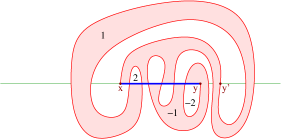
Figure 3: Maslov index and catenation: $x<y<y^{\prime}$.

By Step 2 we may assume ${\varepsilon}_{x}(\Lambda)=1$. Since the orientation of $B^{\prime}$ from $y$ to $y^{\prime}$ is opposite to the orientation of $B$ and the Maslov index of the arc in $B$ from $x$ to $y^{\prime}$ is $-1$, we have

$$\mu(\Lambda)=1-\mu(\Lambda^{\prime}).$$ (18)

Using again the fact that the orientation of $B^{\prime}$ is opposite to the orientation of $B$ we have

$${\varepsilon}_{y}(\Lambda^{\prime})=-{\varepsilon}_{y}(\Lambda),\qquad{\varepsilon}_{y^{\prime}}(\Lambda^{\prime})=-{\varepsilon}_{y^{\prime}}(\Lambda)=1.$$ (19)

Now let $x_{1}<x_{2}<\cdots<x_{m}$ be all intersection points of ${\mathbb{R}}$ and $B$ and let ${\varepsilon}_{i}\in\{-1,+1\}$ be the intersection index of ${\mathbb{R}}$ and $B$ at $x_{i}$. Choose

$$j<k<\ell$$

such that

$$x_{j}=x,\qquad x_{k}=y,\qquad x_{\ell}=y^{\prime}.$$

Then

$${\varepsilon}_{j}={\varepsilon}_{x}(\Lambda)=1,\qquad{\varepsilon}_{k}={\varepsilon}_{y}(\Lambda),\qquad{\varepsilon}_{\ell}={\varepsilon}_{y^{\prime}}(\Lambda)=-1,$$

and

$$k_{x}(\Lambda)=\sum_{i<j}{\varepsilon}_{i},\qquad k_{y}(\Lambda)=-\sum_{i>k}{\varepsilon}_{i}.$$

For $i\neq j$ the intersection index of ${\mathbb{R}}$ and $B^{\prime}$ at $x_{i}$ is $-{\varepsilon}_{i}$. Moreover, $k_{y}(\Lambda^{\prime})$ is the sum of the intersection indices of ${\mathbb{R}}$ and $B^{\prime}$ at all points to the left of $y$ and $k_{y^{\prime}}(\Lambda^{\prime})$ is minus the sum of the intersection indices of ${\mathbb{R}}$ and $B^{\prime}$ at all points to the right of $y^{\prime}$. Hence

$$k_{y}(\Lambda^{\prime})=-\sum_{i<j}{\varepsilon}_{i}-\sum_{j<i<k}{\varepsilon}_{i},\qquad k_{y^{\prime}}(\Lambda^{\prime})=\sum_{i>\ell}{\varepsilon}_{i}.$$

We claim that

$$k_{y^{\prime}}(\Lambda^{\prime})+k_{x}(\Lambda)=0,\qquad k_{y}(\Lambda^{\prime})+k_{y}(\Lambda)=\frac{1+{\varepsilon}_{y}(\Lambda)}{2}.$$ (20)

To see this, note that the value of the winding number ${\rm w}$ slightly to the left of $x$ agrees with the value of ${\rm w}$ slightly to the right of $y^{\prime}$, and hence

$$0=\sum_{i<j}{\varepsilon}_{i}+\sum_{i>\ell}{\varepsilon}_{i}=k_{x}(\Lambda)+k_{y^{\prime}}(\Lambda^{\prime}).$$

This proves the first equation in (20). To prove the second equation in (20) we observe that

$$\sum_{i=1}^{m}{\varepsilon}_{i}=\frac{{\varepsilon}_{x}(\Lambda)+{\varepsilon}_{y}(\Lambda)}{2}$$

and hence

$$k_{y}(\Lambda^{\prime})+k_{y}(\Lambda) = -\sum_{i<j}{\varepsilon}_{i}-\sum_{j<i<k}{\varepsilon}_{i}-\sum_{i>k}{\varepsilon}_{i}$$

$$= {\varepsilon}_{j}+{\varepsilon}_{k}-\sum_{i=1}^{m}{\varepsilon}_{i}$$

$$= {\varepsilon}_{x}(\Lambda)+{\varepsilon}_{y}(\Lambda)-\sum_{i=1}^{m}{\varepsilon}_{i}$$

$$= \frac{{\varepsilon}_{x}(\Lambda)+{\varepsilon}_{y}(\Lambda)}{2}$$

$$= \frac{1+{\varepsilon}_{y}(\Lambda)}{2}.$$

This proves the second equation in (20).

It follows from equation (10) for $\Lambda^{\prime}$ and equations (18), (19), and (20) that

$$\mu(\Lambda) = 1-\mu(\Lambda^{\prime})$$

$$= 1-2k_{y}(\Lambda^{\prime})-2k_{y^{\prime}}(\Lambda^{\prime})-\frac{{\varepsilon}_{y}(\Lambda^{\prime})-{\varepsilon}_{y^{\prime}}(\Lambda^{\prime})}{2}$$

$$= 1-2k_{y}(\Lambda^{\prime})-2k_{y^{\prime}}(\Lambda^{\prime})-\frac{-{\varepsilon}_{y}(\Lambda)-1}{2}$$

$$= 2k_{y}(\Lambda)-{\varepsilon}_{y}(\Lambda)+2k_{x}(\Lambda)+\frac{1+{\varepsilon}_{y}(\Lambda)}{2}$$

$$= 2k_{x}(\Lambda)+2k_{y}(\Lambda)+\frac{1-{\varepsilon}_{y}(\Lambda)}{2}.$$

Here the first equality follows from (18), the second equality follows from (10) for $\Lambda^{\prime}$, the third equality follows from (19), and the fourth equality follows from (20). This proves Step 6.

Step 7. Equation (8) holds when $\Sigma={\mathbb{C}}$ and $\Lambda$ satisfies the arc condition.

It follows from Steps 3-6 by induction that equation (10) holds for every $(\alpha,\beta)$-trace $\Lambda=(x,y,{\rm w})$ whose boundary ${\partial}\Lambda=(x,y,A,B)$ satisfies (11). Hence Step 7 follows from Step 1.

Next we drop the assumption that $\Lambda$ satisfies the arc condition and extend the result to planar surfaces. This requires a further three steps.

Step 8. Equation (8) holds when $\Sigma={\mathbb{C}}$ and $x=y$.

Under these assumptions $\nu_{\alpha}:={\partial}{\rm w}|_{\alpha\setminus\beta}$ and $\nu_{\beta}:=-{\partial}{\rm w}|_{\beta\setminus\alpha}$ are constant. There are four cases.

Case 1. $\alpha$ is an embedded circle and $\beta$ is not an embedded circle. In this case we have $\nu_{\beta}\equiv 0$ and $B=\{x\}$. Moroeover, $\alpha$ is the boundary of a unique disc $\Delta_{\alpha}$ and we assume that $\alpha$ is oriented as the boundary of $\Delta_{\alpha}$. Then the path $\gamma_{\alpha}:[0,1]\to\Sigma$ in Definition 2.1 satisfies $\gamma_{\alpha}(0)=\gamma_{\alpha}(1)=x$ and is homotopic to $\nu_{\alpha}\alpha$. Hence

$$m_{x}(\Lambda)=m_{y}(\Lambda)=2\nu_{\alpha}=\mu(\Lambda).$$

Here the last equation follows from the fact that $\Lambda$ can be obtained as the catenation of $\nu_{\alpha}$ copies of the disc $\Delta_{\alpha}$.

Case 2. $\alpha$ is not an embedded circle and $\beta$ is an embedded circle. This follows from Case 1 by interchanging $\alpha$ and $\beta$.

Case 3. $\alpha$ and $\beta$ are embedded circles. In this case there is a unique pair of embedded discs $\Delta_{\alpha}$ and $\Delta_{\beta}$ with boundaries $\alpha$ and $\beta$, respectively. Orient $\alpha$ and $\beta$ as the boundaries of these discs. Then, for every $z\in\Sigma\setminus\alpha\cup\beta$, we have

$${\rm w}(z)=\left\{\begin{array}[]{ll}\nu_{\alpha}-\nu_{\beta},&\mbox{for }z\in\Delta_{\alpha}\cap\Delta_{\beta},\\ \nu_{\alpha},&\mbox{for }z\in\Delta_{\alpha}\setminus\overline{\Delta}_{\beta},\\ -\nu_{\beta},&\mbox{for }z\in\Delta_{\beta}\setminus\overline{\Delta}_{\alpha},\\ 0,&\mbox{for }z\in\Sigma\setminus\overline{\Delta}_{\alpha}\cup\overline{\Delta}_{\beta}.\end{array}\right.$$

Hence

$$m_{x}(\Lambda)=m_{y}(\Lambda)=2\nu_{\alpha}-2\nu_{\beta}=\mu(\Lambda).$$

Here the last equation follows from the fact $\Lambda$ can be obtained as the catenation of $\nu_{\alpha}$ copies of the disc $\Delta_{\alpha}$ (with the orientation inherited from $\Sigma$) and $\nu_{\beta}$ copies of $-\Delta_{\beta}$ (with the opposite orientation).

Case 4. Neither $\alpha$ nor $\beta$ is an embedded circle. Under this assumption we have $\nu_{\alpha}=\nu_{\beta}=0$. Hence it follows from Theorem 2.4 that ${\rm w}=0$ and $\Lambda=\Lambda_{u}$ for the constant map $u\equiv x\in{\mathcal{D}}(x,x)$. Thus

$$m_{x}(\Lambda)=m_{y}(\Lambda)=\mu(\Lambda)=0.$$

This proves Step 8.

Step 9. Equation (8) holds when $\Sigma={\mathbb{C}}$.

By Step 8, it suffices to assume $x\neq y$. It follows from Theorem 2.4 that every $u\in{\mathcal{D}}(x,y)$ is homotopic to a catentation $u=u_{0}\#v$, where $u_{0}\in{\mathcal{D}}(x,y)$ satisfies the arc condition and $v\in{\mathcal{D}}(y,y)$. Hence it follows from Steps 7 and 8 that

$$\mu(\Lambda_{u}) = \mu(\Lambda_{u_{0}})+\mu(\Lambda_{v})$$

$$= \frac{m_{x}(\Lambda_{u_{0}})+m_{y}(\Lambda_{u_{0}})}{2}+m_{y}(\Lambda_{v})$$

$$= \frac{m_{x}(\Lambda_{u})+m_{y}(\Lambda_{u})}{2}.$$

Here the last equation follows from the fact that ${\rm w}_{u}={\rm w}_{u_{0}}+{\rm w}_{v}$ and hence $m_{z}(\Lambda_{u})=m_{z}(\Lambda_{u_{0}})+m_{z}(\Lambda_{v})$ for every $z\in\alpha\cap\beta$. This proves Step 9.

Step 10. Equation (8) holds when $\Sigma$ is planar.

Choose an element $u\in{\mathcal{D}}(x,y)$ such that $\Lambda_{u}=\Lambda$. Modifying $\alpha$ and $\beta$ on the complement of $u({\mathbb{D}})$, if necessary, we may assume without loss of generality that $\alpha$ and $\beta$ are mebedded circles. Let $\iota:\Sigma\to{\mathbb{C}}$ be an orientation preserving embedding. Then $\iota_{*}\Lambda:=\Lambda_{\iota\circ u}$ is an $(\iota(\alpha),\iota(\beta))$-trace in ${\mathbb{C}}$ and hence satisfies (8) by Step 9. Since $m_{\iota(x)}(\iota_{*}\Lambda)=m_{x}(\Lambda)$, $m_{\iota(y)}(\iota_{*}\Lambda)=m_{y}(\Lambda)$, and $\mu(\iota_{*}\Lambda)=\mu(\Lambda)$ it follows that $\Lambda$ also satisfies (8). This proves Step 10 and Proposition 4.1 ∎

Remark 4.2.

Let $\Lambda=(x,y,A,B)$ be an $(\alpha,\beta)$-trace in ${\mathbb{C}}$ as in Step 1 in the proof of Theorem 3.4. Thus $x<y$ are real numbers, $A$ is the interval $[x,y]$, and $B$ is an embedded arc with endpoints $x,y$ which is oriented from $x$ to $y$ and is transverse to ${\mathbb{R}}$. Thus $Z:=B\cap{\mathbb{R}}$ is a finite set. Define a map

$$f:Z\setminus\{y\}\to Z\setminus\{x\}$$

as follows. Given $z\in Z\setminus\{y\}$ walk along $B$ towards $y$ and let $f(z)$ be the next intersection point with ${\mathbb{R}}$. This map is bijective. Now let $I$ be any of the three open intervals $(-\infty,x)$, $(x,y)$, $(y,\infty)$. Any arc in $B$ from $z$ to $f(z)$ with both endpoints in the same interval $I$ can be removed by an isotopy of $B$ which does not pass through $x,y$. Call $\Lambda$ a reduced $(\alpha,\beta)$-trace if $z\in I$ implies $f(z)\notin I$ for each of the three intervals. Then every $(\alpha,\beta)$-trace is isotopic to a reduced $(\alpha,\beta^{\prime})$-trace and the isotopy does not effect the numbers $\mu,k_{x},k_{y},{\varepsilon}_{x},{\varepsilon}_{y}$.

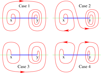
Figure 4: Reduced $(\alpha,\beta)$-traces in ${\mathbb{C}}$.

Let $Z^{+}$ (respectively $Z^{-}$) denote the set of all points $z\in Z=B\cap{\mathbb{R}}$ where the positive tangent vectors in $T_{z}B$ point up (respectively down). One can prove that every reduced $(\alpha,\beta)$-trace satisfies one of the following conditions.

Case 1: If $z\in Z^{+}\setminus\{y\}$ then $f(z)>z$.  Case 2: $Z^{-}\subset[x,y]$.

Case 3: If $z\in Z^{-}\setminus\{y\}$ then $f(z)>z$.  Case 4: $Z^{+}\subset[x,y]$.

(Examples with ${\varepsilon}_{x}=1$ and ${\varepsilon}_{y}=-1$ are depicted in Figure 4.) One can then show directly that the reduced $(\alpha,\beta)$-traces satisfy equation (10). This gives rise to an alternative proof of Proposition 4.1 via case distinction.

Proof of Theorem 3.4 in the Simply Connected Case.

If $\Sigma$ is diffeomorphic to the $2$-plane the result has been established in Proposition 4.1. Hence assume

$$\Sigma=S^{2}.$$

Let $u\in{\mathcal{D}}(x,y)$. If $u$ is not surjective the assertion follows from the case of the complex plane (Proposition 4.1) via stereographic projection. Hence assume $u$ is surjective and choose a regular value $z\in S^{2}\setminus(\alpha\cup\beta)$ of $u$. Denote

$$u^{-1}(z)=\{z_{1},\dots,z_{k}\}.$$

For $i=1,\dots,k$ let ${\varepsilon}_{i}=\pm 1$ according to whether or not the differential $du(z_{i}):{\mathbb{C}}\to T_{z}\Sigma$ is orientation preserving. Choose an open disc $\Delta\subset S^{2}$ centered at $z$ such that

$$\bar{\Delta}\cap(\alpha\cup\beta)=\emptyset$$

and $u^{-1}(\Delta)$ is a union of open neighborhoods $U_{i}\subset{\mathbb{D}}$ of $z_{i}$ with disjoint closures such that

$$u|_{U_{i}}:U_{i}\to\Delta$$

is a diffeomorphism for each $i$ which extends to a neighborhood of $\bar{U}_{i}$. Now choose a continuous map $u^{\prime}:{\mathbb{D}}\to S^{2}$ which agrees with $u$ on ${\mathbb{D}}\setminus\bigcup_{i}U_{i}$ and restricts to a diffeomorphism from $\bar{U}_{i}$ to $S^{2}\setminus\Delta$ for each $i$. Then $z$ does not belong to the image of $u^{\prime}$ and hence equation (8) holds for $u^{\prime}$ (after smoothing along the boundaries ${\partial}U_{i}$). Moreover, the diffeomorphism

$$u^{\prime}|_{\bar{U}_{i}}:\bar{U}_{i}\to S^{2}\setminus\Delta$$

is orientation preserving if and only if ${\varepsilon}_{i}=-1$. Hence

$$\begin{split}\mu(\Lambda_{u})&=\mu(\Lambda_{u^{\prime}})+4\sum_{i=1}^{k}{\varepsilon}_{i},\\ m_{x}(\Lambda_{u})&=m_{x}(\Lambda_{u^{\prime}})+4\sum_{i=1}^{k}{\varepsilon}_{i},\\ m_{y}(\Lambda_{u})&=m_{y}(\Lambda_{u^{\prime}})+4\sum_{i=1}^{k}{\varepsilon}_{i}.\end{split}$$

By Proposition 4.1 equation (8) holds for $\Lambda_{u^{\prime}}$ and hence it also holds for $\Lambda_{u}$. This proves Theorem 3.4 when $\Sigma$ is simply connected. ∎

5 The Non Simply Connected Case

The key step for extending Proposition 4.1 to non-simply connected two-manifolds is the next result about lifts to the universal cover.

Proposition 5.1.

Suppose $\Sigma$ is not diffeomorphic to the $2$-sphere. Let ${\Lambda=(x,y,{\rm w})}$ be an $(\alpha,\beta)$-trace and ${\pi:{\mathbb{C}}\to\Sigma}$ be a universal covering. Denote by $\Gamma\subset{\rm Diff}({\mathbb{C}})$ the group of deck transformations. Choose an element ${{\tilde{x}}\in\pi^{-1}(x)}$ and let ${\tilde{\alpha}}$ and ${\tilde{\beta}}$ be the lifts of $\alpha$ and $\beta$ through ${\tilde{x}}$. Let ${\tilde{\Lambda}}=({\tilde{x}},{\tilde{y}},\tilde{\rm w})$ be the lift of $\Lambda$ with left endpoint ${\tilde{x}}$. Then

$$m_{g{\tilde{x}}}({\tilde{\Lambda}})+m_{g^{-1}{\tilde{y}}}({\tilde{\Lambda}})=0$$ (21)

for every $g\in\Gamma\setminus\{{\rm id}\}$.

Lemma 5.2 (Annulus Reduction).

Suppose $\Sigma$ is not diffeomorphic to the $2$-sphere. Let $\Lambda$, $\pi$, $\Gamma$, ${\tilde{\Lambda}}$ be as in Proposition 5.1. If

$$m_{g{\tilde{x}}}({\tilde{\Lambda}})-m_{g{\tilde{y}}}({\tilde{\Lambda}})=m_{g^{-1}{\tilde{y}}}({\tilde{\Lambda}})-m_{g^{-1}{\tilde{x}}}({\tilde{\Lambda}})$$ (22)

for every $g\in\Gamma\setminus\{{\rm id}\}$ then equation (21) holds for every $g\in\Gamma\setminus\{{\rm id}\}$.

Proof.

If (21) does not hold then there is a deck transformation $h\in\Gamma\setminus\{{\rm id}\}$ such that $m_{h{\tilde{x}}}({\tilde{\Lambda}})+m_{h^{-1}{\tilde{y}}}({\tilde{\Lambda}})\neq 0.$ Since there can only be finitely many such $h\in\Gamma\setminus\{{\rm id}\}$, there is an integer $k\geq 1$ such that $m_{h^{k}{\tilde{x}}}({\tilde{\Lambda}})+m_{h^{-k}{\tilde{y}}}({\tilde{\Lambda}})\neq 0$ and $m_{h^{\ell}{\tilde{x}}}({\tilde{\Lambda}})+m_{h^{-\ell}{\tilde{y}}}({\tilde{\Lambda}})=0$ for every integer $\ell>k$. Define $g:=h^{k}$. Then

$$m_{g{\tilde{x}}}({\tilde{\Lambda}})+m_{g^{-1}{\tilde{y}}}({\tilde{\Lambda}})\neq 0$$ (23)

and $m_{g^{k}{\tilde{x}}}({\tilde{\Lambda}})+m_{g^{-k}{\tilde{y}}}({\tilde{\Lambda}})=0$ for every integer $k\in{\mathbb{Z}}\setminus\{-1,0,1\}$. Define

$$\Sigma_{0}:={\mathbb{C}}/\Gamma_{0},\qquad\Gamma_{0}:=\left\{g^{k}\,|\,k\in{\mathbb{Z}}\right\}.$$

Then $\Sigma_{0}$ is diffeomorphic to the annulus. Let $\pi_{0}:{\mathbb{C}}\to\Sigma_{0}$ be the obvious projection, define $\alpha_{0}:=\pi_{0}({\tilde{\alpha}})$, $\beta_{0}:=\pi_{0}({\tilde{\beta}})$, and let $\Lambda_{0}:=(x_{0},y_{0},{\rm w}_{0})$ be the $(\alpha_{0},\beta_{0})$-trace in $\Sigma_{0}$ with $x_{0}:=\pi_{0}({\tilde{x}})$, $y_{0}:=\pi_{0}({\tilde{y}})$, and

$${\rm w}_{0}(z_{0}):=\sum_{{\tilde{z}}\in\pi_{0}^{-1}(z_{0})}\tilde{\rm w}({\tilde{z}}),\qquad z_{0}\in\Sigma_{0}\setminus(\alpha_{0}\cup\beta_{0}).$$

Then

$$\begin{split}m_{x_{0}}(\Lambda_{0})&=m_{\tilde{x}}({\tilde{\Lambda}})+\sum_{k\in{\mathbb{Z}}\setminus\{0\}}m_{g^{k}{\tilde{x}}}({\tilde{\Lambda}}),\\ m_{y_{0}}(\Lambda_{0})&=m_{\tilde{y}}({\tilde{\Lambda}})+\sum_{k\in{\mathbb{Z}}\setminus\{0\}}m_{g^{-k}{\tilde{y}}}({\tilde{\Lambda}}).\end{split}$$

By Proposition 4.1 both ${\tilde{\Lambda}}$ and $\Lambda_{0}$ satisfy equation (8) and they have the same Viterbo–Maslov index. Hence

$$0 = \mu(\Lambda_{0})-\mu({\tilde{\Lambda}})$$

$$= \frac{m_{x_{0}}(\Lambda_{0})+m_{y_{0}}(\Lambda_{0})}{2}-\frac{m_{\tilde{x}}({\tilde{\Lambda}})+m_{\tilde{y}}({\tilde{\Lambda}})}{2}$$

$$= \frac{1}{2}\sum_{k\neq 0}\left(m_{g^{k}{\tilde{x}}}({\tilde{\Lambda}})+m_{g^{-k}{\tilde{y}}}({\tilde{\Lambda}})\right)$$

$$= m_{g{\tilde{x}}}({\tilde{\Lambda}})+m_{g^{-1}{\tilde{y}}}({\tilde{\Lambda}}).$$

Here the last equation follows from (22). This contradicts (23) and proves Lemma 5.2. ∎

Lemma 5.3.

Suppose $\Sigma$ is not diffeomorphic to the $2$-sphere. Let $\Lambda$, $\pi$, $\Gamma$, ${\tilde{\Lambda}}$ be as in Proposition 5.1 and denote $\nu_{\tilde{\alpha}}:={\partial}\tilde{\rm w}|_{{\tilde{\alpha}}\setminus{\tilde{\beta}}}$ and $\nu_{\tilde{\beta}}:=-{\partial}\tilde{\rm w}|_{{\tilde{\beta}}\setminus{\tilde{\alpha}}}$. Choose smooth paths

$$\gamma_{\tilde{\alpha}}:[0,1]\to{\tilde{\alpha}},\qquad\gamma_{\tilde{\beta}}:[0,1]\to{\tilde{\beta}}$$

from $\gamma_{\tilde{\alpha}}(0)=\gamma_{\tilde{\beta}}(0)={\tilde{x}}$ to $\gamma_{\tilde{\alpha}}(1)=\gamma_{\tilde{\beta}}(1)={\tilde{y}}$ such that $\gamma_{\tilde{\alpha}}$ is an immersion when $\nu_{\tilde{\alpha}}\not\equiv 0$ and constant when $\nu_{\tilde{\alpha}}\equiv 0$, the same holds for $\gamma_{\tilde{\beta}}$, and

$$\begin{split}\nu_{\tilde{\alpha}}({\tilde{z}})=\deg(\gamma_{\tilde{\alpha}},{\tilde{z}})&\quad\mbox{for}\quad{\tilde{z}}\in{\tilde{\alpha}}\setminus\{{\tilde{x}},{\tilde{y}}\},\\ \nu_{\tilde{\beta}}({\tilde{z}})=\deg(\gamma_{\tilde{\beta}},{\tilde{z}})&\quad\mbox{for}\quad{\tilde{z}}\in{\tilde{\beta}}\setminus\{{\tilde{x}},{\tilde{y}}\}.\end{split}$$

Define

$${\tilde{A}}:=\gamma_{\tilde{\alpha}}([0,1]),\qquad{\tilde{B}}:=\gamma_{\tilde{\beta}}([0,1]).$$

Then, for every $g\in\Gamma$, we have

$$g{\tilde{x}}\in{\tilde{A}}\qquad\iff\qquad g^{-1}{\tilde{y}}\in{\tilde{A}},$$ (24)

$$g{\tilde{x}}\notin{\tilde{A}}\;\;\mbox{ and }\;\;g{\tilde{y}}\notin{\tilde{A}}\qquad\iff\qquad{\tilde{A}}\cap g{\tilde{A}}=\emptyset,$$ (25)

$$g{\tilde{x}}\in{\tilde{A}}\;\;\mbox{ and }\;\;g{\tilde{y}}\in{\tilde{A}}\qquad\iff\qquad g={\rm id}.$$ (26)

The same holds with ${\tilde{A}}$ replaced by ${\tilde{B}}$.

Proof.

If $\alpha$ is a contractible embedded circle or not an embedded circle at all we have ${\tilde{A}}\cap g{\tilde{A}}=\emptyset$ whenever $g\neq{\rm id}$ and this implies (24), (25) and (26). Hence assume $\alpha$ is a noncontractible embedded circle. Then we may also assume, without loss of generality, that $\pi({\mathbb{R}})=\alpha$, the map ${\tilde{z}}\mapsto{\tilde{z}}+1$ is a deck transformation, $\pi$ maps the interval $[0,1)$ bijectively onto $\alpha$, and ${\tilde{x}},{\tilde{y}}\in{\mathbb{R}}={\tilde{\alpha}}$ with ${\tilde{x}}<{\tilde{y}}$. Thus ${\tilde{A}}=[{\tilde{x}},{\tilde{y}}]$ and, for every $k\in{\mathbb{Z}}$,

$${\tilde{x}}+k\in[{\tilde{x}},{\tilde{y}}]\quad\iff\quad 0\leq k\leq{\tilde{y}}-{\tilde{x}}\quad\iff\quad{\tilde{y}}-k\in[{\tilde{x}},{\tilde{y}}].$$

Similarly, we have

$${\tilde{x}}+k,{\tilde{y}}+k\notin[{\tilde{x}},{\tilde{y}}]\quad\iff\quad[{\tilde{x}}+k,{\tilde{y}}+k]\cap[{\tilde{x}},{\tilde{y}}]=\emptyset$$

and

$${\tilde{x}}+k,{\tilde{y}}+k\in[{\tilde{x}},{\tilde{y}}]\quad\iff\quad[{\tilde{x}}+k,{\tilde{y}}+k]\subset[{\tilde{x}},{\tilde{y}}]\quad\iff\quad k=0.$$

This proves (24), (25), and (26) for the deck transformation ${\tilde{z}}\mapsto{\tilde{z}}+k$. If $g$ is any other deck transformation, then we have

$${\tilde{\alpha}}\cap g{\tilde{\alpha}}=\emptyset$$

and so (24), (25), and (26) are trivially satisfied. This proves Lemma 5.3. ∎

Lemma 5.4 (Winding Number Comparison).

Suppose $\Sigma$ is not diffeomorphic to the $2$-sphere. Let $\Lambda$, $\pi$, $\Gamma$, ${\tilde{\Lambda}}$ be as in Proposition 5.1, and let ${\tilde{A}},{\tilde{B}}\subset{\mathbb{C}}$ be as in Lemma 5.3. Then the following holds.

(i) Equation (22) holds for every $g\in\Gamma$ that satisfies $g{\tilde{x}},g{\tilde{y}}\notin{\tilde{A}}\cup{\tilde{B}}$.

(ii) If $\Lambda$ satisfies the arc condition then (21) holds for every $g\in\Gamma\setminus\{{\rm id}\}$.

Proof.

We prove (i). Let $g\in\Gamma$ such that $g{\tilde{x}},g{\tilde{y}}\notin{\tilde{A}}\cup{\tilde{B}}$ and let $\gamma_{\tilde{\alpha}},\gamma_{\tilde{\beta}}$ be as in Lemma 5.3. Then $\tilde{\rm w}({\tilde{z}})$ is the winding number of the loop $\gamma_{\tilde{\alpha}}-\gamma_{\tilde{\beta}}$ about the point ${\tilde{z}}\in{\mathbb{C}}\setminus({\tilde{A}}\cup{\tilde{B}})$. Moreover, the paths

$$g\gamma_{\tilde{\alpha}}:[0,1]\to{\mathbb{C}},\qquad g\gamma_{\tilde{\beta}}:[0,1]\to{\mathbb{C}}$$

connect the points $g{\tilde{x}},g{\tilde{y}}\in{\mathbb{C}}\setminus({\tilde{A}}\cup{\tilde{B}})$. Hence

$$\tilde{\rm w}(g{\tilde{y}})-\tilde{\rm w}(g{\tilde{x}})=(\gamma_{\tilde{\alpha}}-\gamma_{\tilde{\beta}})\cdot g\gamma_{\tilde{\alpha}}=(\gamma_{\tilde{\alpha}}-\gamma_{\tilde{\beta}})\cdot g\gamma_{\tilde{\beta}}.$$

Similarly with $g$ replaced by $g^{-1}$. Moreover, it follows from Lemma 5.3, that

$${\tilde{A}}\cap g{\tilde{A}}=\emptyset,\qquad{\tilde{B}}\cap g^{-1}{\tilde{B}}=\emptyset.$$

Hence

$$\tilde{\rm w}(g{\tilde{y}})-\tilde{\rm w}(g{\tilde{x}}) = \left(\gamma_{\tilde{\alpha}}-\gamma_{\tilde{\beta}}\right)\cdot g\gamma_{\tilde{\alpha}}$$

$$= g\gamma_{\tilde{\alpha}}\cdot\gamma_{\tilde{\beta}}$$

$$= \gamma_{\tilde{\alpha}}\cdot g^{-1}\gamma_{\tilde{\beta}}$$

$$= \left(\gamma_{\tilde{\alpha}}-\gamma_{\tilde{\beta}}\right)\cdot g^{-1}\gamma_{\tilde{\beta}}$$

$$= \tilde{\rm w}(g^{-1}{\tilde{y}})-\tilde{\rm w}(g^{-1}{\tilde{x}})$$

Here we have used the fact that every $g\in\Gamma$ is an orientation preserving diffeomorphism of ${\mathbb{C}}$. Thus we have proved that

$$\tilde{\rm w}(g{\tilde{x}})+\tilde{\rm w}(g^{-1}{\tilde{y}})=\tilde{\rm w}(g{\tilde{y}})+\tilde{\rm w}(g^{-1}{\tilde{x}}).$$

Since $g{\tilde{x}},g{\tilde{y}}\notin{\tilde{A}}\cup{\tilde{B}}$, we have

$$m_{g{\tilde{x}}}({\tilde{\Lambda}})=4\tilde{\rm w}(g{\tilde{x}}),\qquad m_{g^{-1}{\tilde{y}}}({\tilde{\Lambda}})=4\tilde{\rm w}(g^{-1}{\tilde{y}}),$$

and the same identities hold with $g$ replaced by $g^{-1}$. This proves (i).

We prove (ii). If $\Lambda$ satisfies the arc condition then $g{\tilde{A}}\cap{\tilde{A}}=\emptyset$ and $g{\tilde{B}}\cap{\tilde{B}}=\emptyset$ for every $g\in\Gamma\setminus\{{\rm id}\}$. In particular, for every $g\in\Gamma\setminus\{{\rm id}\}$, we have $g{\tilde{x}},g{\tilde{y}}\notin{\tilde{A}}\cup{\tilde{B}}$ and hence (22) holds by (i). Hence it follows from Lemma 5.2 that (21) holds for every $g\in\Gamma\setminus\{{\rm id}\}$. This proves Lemma 5.4. ∎

The next lemma deals with $(\alpha,\beta)$-traces connecting a point $x\in\alpha\cap\beta$ to itself. An example on the annulus is depicted in Figure 5.

Lemma 5.5 (Isotopy Argument).

Suppose $\Sigma$ is not diffeomorphic to the $2$-sphere. Let $\Lambda$, $\pi$, $\Gamma$, ${\tilde{\Lambda}}$ be as in Proposition 5.1. Suppose that there is a deck transformation $g_{0}\in\Gamma\setminus\{{\rm id}\}$ such that ${\tilde{y}}=g_{0}{\tilde{x}}$. Then $\Lambda$ has Viterbo–Maslov index zero and $m_{g{\tilde{x}}}({\tilde{\Lambda}})=0$ for every $g\in\Gamma\setminus\{{\rm id},g_{0}\}$.

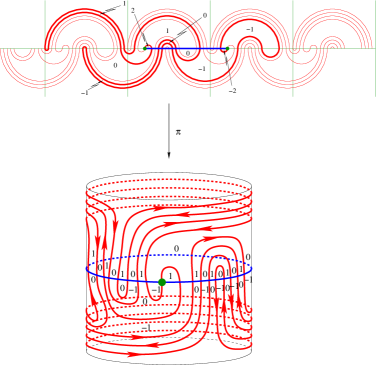
Figure 5: An $(\alpha,\beta)$-trace on the annulus with $x=y$.

Proof.

By assumption, we have ${\tilde{\alpha}}=g_{0}{\tilde{\alpha}}$ and ${\tilde{\beta}}=g_{0}{\tilde{\beta}}$. Hence $\alpha$ and $\beta$ are noncontractible embedded circles and some iterate of $\alpha$ is homotopic to some iterate of $\beta$. Hence, by Lemma A.4, $\alpha$ must be homotopic to $\beta$ (with some orientation). Hence we may assume, without loss of generality, that $\pi({\mathbb{R}})=\alpha$, the map ${\tilde{z}}\mapsto{\tilde{z}}+1$ is a deck transformation, $\pi$ maps the interval $[0,1)$ bijectively onto $\alpha$, ${\mathbb{R}}={\tilde{\alpha}}$, ${\tilde{x}}=0\in{\tilde{\alpha}}\cap{\tilde{\beta}}$, ${\tilde{\beta}}={\tilde{\beta}}+1$, and that ${\tilde{y}}=\ell>0$ is an integer. Then $g_{0}$ is the translation

$$g_{0}({\tilde{z}})={\tilde{z}}+\ell.$$

Let ${\tilde{A}}:=[0,\ell]\subset{\tilde{\alpha}}$ and let ${\tilde{B}}\subset{\tilde{\beta}}$ be the arc connecting $0$ to $\ell$. Then, for ${\tilde{z}}\in{\mathbb{C}}\setminus({\tilde{A}}\cup{\tilde{B}})$, the integer $\tilde{\rm w}({\tilde{z}})$ is the winding number of ${\tilde{A}}-{\tilde{B}}$ about ${\tilde{z}}$. Define the projection $\pi_{0}:{\mathbb{C}}\to{\mathbb{C}}$ by

$$\pi_{0}({\tilde{z}}):=e^{2\pi{\mathbf{i}}{\tilde{z}}/k},$$

denote $\alpha_{0}:=\pi_{0}({\tilde{\alpha}})=S^{1}$ and $\beta_{0}:=\pi({\tilde{\beta}})$, and let $\Lambda_{0}=(1,1,{\rm w}_{0})$ be the induced $(\alpha_{0},\beta_{0})$-trace in ${\mathbb{C}}$ with ${\rm w}_{0}(z):=\sum_{{\tilde{z}}\in\pi^{-1}(z)}\tilde{\rm w}({\tilde{z}}).$ Then $\alpha_{0}$ and $\beta_{0}$ are embedded circles and have the winding number $\ell$ about zero. Hence it follows from Step 8, Case 3 in the proof of Proposition 4.1 that $\Lambda_{0}$ has Viterbo–Maslov index zero and satisfies $m_{x_{0}}(\Lambda_{0})+m_{y_{0}}(\Lambda_{0})=2\mu(\Lambda_{0})=0$. Hence ${\tilde{\Lambda}}$ also has Viterbo–Maslov index zero.

It remains to prove that $m_{g{\tilde{x}}}({\tilde{\Lambda}})=0$ for every $g\in\Gamma\setminus\{{\rm id},g_{0}\}$. To see this we use the fact that the embedded loops $\alpha$ and $\beta$ are homotopic with fixed endpoint $x$. Hence, by a Theorem of Epstein, they are isotopic with fixed basepoint $x$ (see [2, Theorem 4.1]). Thus there exists a smooth map $f:{\mathbb{R}}/{\mathbb{Z}}\times[0,1]\to\Sigma$ such that

$$f(s,0)\in\alpha,\qquad f(s,1)\in\beta,\qquad f(0,t)=x,$$

for all $s\in{\mathbb{R}}/{\mathbb{Z}}$ and $t\in[0,1]$, and the map ${\mathbb{R}}/{\mathbb{Z}}\to\Sigma:s\mapsto f(s,t)$ is an embedding for every $s\in[0,1]$. Lift this homotopy to the universal cover to obtain a map ${\tilde{f}}:{\mathbb{R}}\times[0,1]\to{\mathbb{C}}$ such that $\pi\circ{\tilde{f}}=f$ and

$${\tilde{f}}(s,0)\in[0,1],\quad{\tilde{f}}(s,1)\in{\tilde{B}}_{1},\quad{\tilde{f}}(0,t)={\tilde{x}},\quad{\tilde{f}}(s+1,t)={\tilde{f}}(s,t)+1$$

for all $s\in{\mathbb{R}}$ and $t\in[0,1]$. Here ${\tilde{B}}_{1}\subset{\tilde{B}}$ denotes the arc in ${\tilde{B}}$ from $0$ to $1$. Since the map ${\mathbb{R}}/{\mathbb{Z}}\to\Sigma:s\mapsto f(s,t)$ is injective for every $t$, we have

$$g{\tilde{x}}\notin\{{\tilde{x}},{\tilde{x}}+1,\dots,{\tilde{x}}+\ell\}\qquad\implies\qquad g{\tilde{x}}\notin{\tilde{f}}([0,\ell]\times[0,1])$$

for every every $g\in\Gamma$. Now choose a smooth map ${\tilde{u}}:{\mathbb{D}}\to{\mathbb{C}}$ with $\Lambda_{\tilde{u}}={\tilde{\Lambda}}$ (see Theorem 2.4). Define the homotopy $F_{\tilde{u}}:[0,\ell]\times[0,1]\to{\mathbb{C}}$ by $F_{\tilde{u}}(s,t):={\tilde{u}}(-\cos(\pi s/\ell),t\sin(\pi s/\ell))$. Then, by Theorem 2.4, $F_{\tilde{u}}$ is homotopic to ${\tilde{f}}|_{[0,\ell]\times[0,1]}$ subject to the boundary conditions ${\tilde{f}}(s,0)\in{\tilde{\alpha}}={\mathbb{R}}$, ${\tilde{f}}(s,1)\in{\tilde{\beta}}$, ${\tilde{f}}(0,t)={\tilde{x}}$, ${\tilde{f}}(\ell,t)={\tilde{y}}$. Hence, for every ${\tilde{z}}\in{\mathbb{C}}\setminus({\tilde{\alpha}}\cup{\tilde{\beta}})$, we have

$$\tilde{\rm w}({\tilde{z}})=\deg({\tilde{u}},z)=\deg(F_{\tilde{u}},{\tilde{z}})=\deg({\tilde{f}},{\tilde{z}}).$$

In particular, choosing ${\tilde{z}}$ near $g{\tilde{x}}$, we find $m_{g{\tilde{x}}}({\tilde{\Lambda}})=4\deg({\tilde{f}},g{\tilde{x}})=0$ for every $g\in\Gamma$ that is not one of the translations ${\tilde{z}}\mapsto{\tilde{z}}+k$ for $k=0,1,\dots,\ell$. This proves the assertion in the case $\ell=1$.

If $\ell>1$ it remains to prove $m_{k}({\tilde{\Lambda}})=0$ for $k=1,\dots,\ell-1$. To see this, let ${\tilde{A}}_{1}:=[0,1]$, ${\tilde{B}}_{1}\subset{\tilde{B}}$ be the arc from $0$ to $1$, $\tilde{\rm w}_{1}({\tilde{z}})$ be the winding number of ${\tilde{A}}_{1}-{\tilde{B}}_{1}$ about ${\tilde{z}}\in{\mathbb{C}}\setminus({\tilde{A}}_{1}\cup{\tilde{B}}_{1})$, and define ${\tilde{\Lambda}}_{1}:=(0,1,\tilde{\rm w}_{1}).$ Then, by what we have already proved, the $({\tilde{\alpha}},{\tilde{\beta}})$-trace ${\tilde{\Lambda}}_{1}$ satisfies $m_{g{\tilde{x}}}({\tilde{\Lambda}}_{1})=0$ for every $g\in\Gamma$ other than the translations by $0$ or $1$. In particular, we have $m_{j}({\tilde{\Lambda}}_{1})=0$ for every $j\in{\mathbb{Z}}\setminus\{0,1\}$ and also $m_{0}({\tilde{\Lambda}}_{1})+m_{1}({\tilde{\Lambda}}_{1})=2\mu({\tilde{\Lambda}}_{1})=0$. Since $\tilde{\rm w}({\tilde{z}})=\sum_{j=0}^{\ell-1}\tilde{\rm w}_{1}({\tilde{z}}-j)$ for ${\tilde{z}}\in{\mathbb{C}}\setminus({\tilde{A}}\cup{\tilde{B}})$, we obtain

$$m_{k}({\tilde{\Lambda}})=\sum_{j=0}^{\ell-1}m_{k-j}({\tilde{\Lambda}}_{1})=0$$

for every $k\in{\mathbb{Z}}\setminus\{0,\ell\}$. This proves Lemma 5.5. ∎

The next example shows that Lemma 5.4 cannot be strengthened to assert the identity $m_{g{\tilde{x}}}({\tilde{\Lambda}})=0$ for every $g\in\Gamma$ with $g{\tilde{x}},g{\tilde{y}}\notin{\tilde{A}}\cup{\tilde{B}}$.

Example 5.6.

Figure 6 depicts an $(\alpha,\beta)$-trace $\Lambda=(x,y,{\rm w})$ on the annulus $\Sigma={\mathbb{C}}/{\mathbb{Z}}$ that has Viterbo–Maslov index one and satisfies the arc condition. The lift satisfies $m_{\tilde{x}}({\tilde{\Lambda}})=-3$, $m_{{\tilde{x}}+1}({\tilde{\Lambda}})=4$, $m_{{\tilde{y}}}({\tilde{\Lambda}})=5$, and $m_{{\tilde{y}}-1}({\tilde{\Lambda}})=-4$. Thus $m_{x}(\Lambda)=m_{y}(\Lambda)=1$.

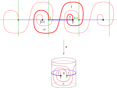
Figure 6: An $(\alpha,\beta)$-trace on the annulus satisfying the arc condition.

Proof of Proposition 5.1.

The proof has five steps.

Step 1. Let ${\tilde{A}},{\tilde{B}}\subset{\mathbb{C}}$ be as in Lemma 5.3 and let $g\in\Gamma$ such that

$$g{\tilde{x}}\in{\tilde{A}}\setminus{\tilde{B}},\qquad g{\tilde{y}}\notin{\tilde{A}}\cup{\tilde{B}}.$$

(An example is depicted in Figure 7.) Then (22) holds.

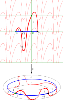
Figure 7: An $(\alpha,\beta)$-trace on the torus not satisfying the arc condition.

The proof is a refinement of the winding number comparison argument in Lemma 5.4. Since $g{\tilde{x}}\notin{\tilde{B}}$ we have $g\neq{\rm id}$ and, since ${\tilde{x}},g{\tilde{x}}\in{\tilde{A}}\subset{\tilde{\alpha}}$, it follows that $\alpha$ is a noncontractible embedded circle. Hence we may choose the universal covering $\pi:{\mathbb{C}}\to\Sigma$ and the lifts ${\tilde{\alpha}}$, ${\tilde{\beta}}$, ${\tilde{\Lambda}}$ such that $\pi({\mathbb{R}})=\alpha$, the map ${\tilde{z}}\mapsto{\tilde{z}}+1$ is a deck transformation, the projection $\pi$ maps the interval $[0,1)$ bijectively onto $\alpha$, and

$${\tilde{\alpha}}={\mathbb{R}},\qquad{\tilde{x}}=0\in{\tilde{\alpha}}\cap{\tilde{\beta}},\qquad{\tilde{y}}>0.$$

By assumption and Lemma 5.3 there is an integer $k$ such that

$$0<k<{\tilde{y}},\qquad g{\tilde{x}}=k,\qquad g^{-1}{\tilde{y}}={\tilde{y}}-k.$$

Thus $g$ is the deck transformation ${\tilde{z}}\mapsto{\tilde{z}}+k$.

Since $g{\tilde{x}}\notin{\tilde{B}}$ and $g{\tilde{y}}\notin{\tilde{B}}$ it follows from Lemma 5.3 that $g^{-1}{\tilde{y}}\notin{\tilde{B}}$ and $g^{-1}{\tilde{x}}\notin{\tilde{B}}$ and hence, again by Lemma 5.3, we have

$${\tilde{B}}\cap g{\tilde{B}}={\tilde{B}}\cap g^{-1}{\tilde{B}}=\emptyset.$$

With $\gamma_{\tilde{\alpha}}$ and $\gamma_{\tilde{\beta}}$ chosen as in Lemma 5.3, this implies

$$\gamma_{\tilde{\beta}}\cdot(\gamma_{\tilde{\beta}}-k)=(\gamma_{\tilde{\beta}}+k)\cdot\gamma_{\tilde{\beta}}=0.$$ (27)

Since $k,-k,{\tilde{y}}+k,{\tilde{y}}-k\notin{\tilde{B}}$, there exists a constant ${\varepsilon}>0$ such that

$$-{\varepsilon}\leq t\leq{\varepsilon}\qquad\implies\qquad k+{\mathbf{i}}t,\;\;-k+{\mathbf{i}}t,\;\;{\tilde{y}}-k+{\mathbf{i}}t,\;\;{\tilde{y}}+k+{\mathbf{i}}t\notin{\tilde{B}}.$$

The paths $g\gamma_{\tilde{\alpha}}\pm{\mathbf{i}}{\varepsilon}$ and $g\gamma_{\tilde{\beta}}\pm{\mathbf{i}}{\varepsilon}$ both connect the point $g{\tilde{x}}\pm{\mathbf{i}}{\varepsilon}$ to $g{\tilde{y}}\pm{\mathbf{i}}{\varepsilon}$. Likewise, the paths $g^{-1}\gamma_{\tilde{\alpha}}\pm{\mathbf{i}}{\varepsilon}$ and $g^{-1}\gamma_{\tilde{\beta}}\pm{\mathbf{i}}{\varepsilon}$ both connect the point $g^{-1}{\tilde{x}}\pm{\mathbf{i}}{\varepsilon}$ to $g^{-1}{\tilde{y}}\pm{\mathbf{i}}{\varepsilon}$. Hence

$$\tilde{\rm w}(g{\tilde{y}}\pm{\mathbf{i}}{\varepsilon})-\tilde{\rm w}(g{\tilde{x}}\pm{\mathbf{i}}{\varepsilon}) = (\gamma_{\tilde{\alpha}}-\gamma_{\tilde{\beta}})\cdot(g\gamma_{\tilde{\alpha}}\pm{\mathbf{i}}{\varepsilon})$$

$$= (\gamma_{\tilde{\alpha}}-\gamma_{\tilde{\beta}})\cdot(\gamma_{\tilde{\alpha}}+k\pm{\mathbf{i}}{\varepsilon})$$

$$= (\gamma_{\tilde{\alpha}}+k\pm{\mathbf{i}}{\varepsilon})\cdot\gamma_{\tilde{\beta}}$$

$$= \gamma_{\tilde{\alpha}}\cdot(\gamma_{\tilde{\beta}}-k\mp{\mathbf{i}}{\varepsilon})$$

$$= (\gamma_{\tilde{\alpha}}-\gamma_{\tilde{\beta}})\cdot(\gamma_{\tilde{\beta}}-k\mp{\mathbf{i}}{\varepsilon})$$

$$= (\gamma_{\tilde{\alpha}}-\gamma_{\tilde{\beta}})\cdot(g^{-1}\gamma_{\tilde{\beta}}\mp{\mathbf{i}}{\varepsilon})$$

$$= \tilde{\rm w}(g^{-1}{\tilde{y}}\mp{\mathbf{i}}{\varepsilon})-\tilde{\rm w}(g^{-1}{\tilde{x}}\mp{\mathbf{i}}{\varepsilon}).$$

Here the last but one equation follows from (27). Thus we have proved

$$\begin{split}\tilde{\rm w}(g{\tilde{x}}+{\mathbf{i}}{\varepsilon})+\tilde{\rm w}(g^{-1}{\tilde{y}}-{\mathbf{i}}{\varepsilon})&=\tilde{\rm w}(g^{-1}{\tilde{x}}-{\mathbf{i}}{\varepsilon})+\tilde{\rm w}(g{\tilde{y}}+{\mathbf{i}}{\varepsilon}),\\ \tilde{\rm w}(g{\tilde{x}}-{\mathbf{i}}{\varepsilon})+\tilde{\rm w}(g^{-1}{\tilde{y}}+{\mathbf{i}}{\varepsilon})&=\tilde{\rm w}(g^{-1}{\tilde{x}}+{\mathbf{i}}{\varepsilon})+\tilde{\rm w}(g{\tilde{y}}-{\mathbf{i}}{\varepsilon}).\end{split}$$ (28)

Since

$$\begin{split}m_{g{\tilde{x}}}({\tilde{\Lambda}})&=2\tilde{\rm w}(g{\tilde{x}}+{\mathbf{i}}{\varepsilon})+2\tilde{\rm w}(g{\tilde{x}}-{\mathbf{i}}{\varepsilon}),\\ m_{g{\tilde{y}}}({\tilde{\Lambda}})&=2\tilde{\rm w}(g{\tilde{y}}+{\mathbf{i}}{\varepsilon})+2\tilde{\rm w}(g{\tilde{y}}-{\mathbf{i}}{\varepsilon}),\\ m_{g^{-1}{\tilde{x}}}({\tilde{\Lambda}})&=2\tilde{\rm w}(g^{-1}{\tilde{x}}+{\mathbf{i}}{\varepsilon})+2\tilde{\rm w}(g^{-1}{\tilde{x}}-{\mathbf{i}}{\varepsilon}),\\ m_{g^{-1}{\tilde{y}}}({\tilde{\Lambda}})&=2\tilde{\rm w}(g^{-1}{\tilde{y}}+{\mathbf{i}}{\varepsilon})+2\tilde{\rm w}(g^{-1}{\tilde{y}}-{\mathbf{i}}{\varepsilon}),\end{split}$$

Step 1 follows by taking the sum of the two equations in (28).

Step 2. Let ${\tilde{A}},{\tilde{B}}\subset{\mathbb{C}}$ be as in Lemma 5.3 and let $g\in\Gamma$. Suppose that either $g{\tilde{x}},g{\tilde{y}}\notin{\tilde{A}}$ or $g{\tilde{x}},g{\tilde{y}}\notin{\tilde{B}}$. Then (22) holds.

If $g{\tilde{x}},g{\tilde{y}}\notin{\tilde{A}}\cup{\tilde{B}}$ the assertion follows from Lemma 5.4. If $g{\tilde{x}}\in{\tilde{A}}\setminus{\tilde{B}}$ and $g{\tilde{y}}\notin{\tilde{A}}\cup{\tilde{B}}$ the assertion follows from Step 1. If $g{\tilde{x}}\notin{\tilde{A}}\cup{\tilde{B}}$ and $g{\tilde{y}}\in{\tilde{A}}\setminus{\tilde{B}}$ the assertion follows from Step 1 by interchanging ${\tilde{x}}$ and ${\tilde{y}}$. Namely, (22) holds for ${\tilde{\Lambda}}$ if and only if it holds for the $({\tilde{\alpha}},{\tilde{\beta}})$-trace $-{\tilde{\Lambda}}:=({\tilde{y}},{\tilde{x}},-\tilde{\rm w}).$ This covers the case $g{\tilde{x}},g{\tilde{y}}\notin{\tilde{B}}$. If $g{\tilde{x}},g{\tilde{y}}\notin{\tilde{A}}$ the assertion follows by interchanging ${\tilde{A}}$ and ${\tilde{B}}$. Namely, (22) holds for ${\tilde{\Lambda}}$ if and only if it holds for the $({\tilde{\beta}},{\tilde{\alpha}})$-trace ${\tilde{\Lambda}}^{*}:=({\tilde{x}},{\tilde{y}},-\tilde{\rm w}).$ This proves Step 2.

Step 3. Let ${\tilde{A}},{\tilde{B}}\subset{\mathbb{C}}$ be as in Lemma 5.3 and let $g\in\Gamma$ such that

$$g{\tilde{x}}\in{\tilde{A}}\setminus{\tilde{B}},\qquad g{\tilde{y}}\in{\tilde{B}}\setminus{\tilde{A}}.$$

(An example is depicted in Figure 8.) Then (21) holds for $g$ and $g^{-1}$.

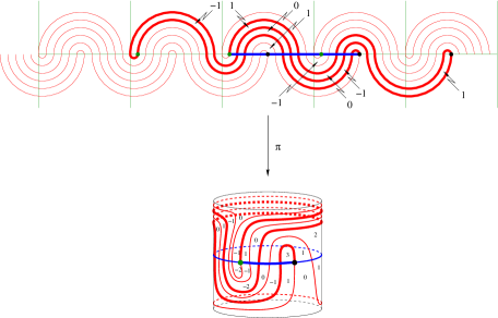
Figure 8: An $(\alpha,\beta)$-trace on the annulus with $g{\tilde{x}}\in{\tilde{A}}$ and $g{\tilde{y}}\in{\tilde{B}}$.

Since $g{\tilde{x}}\notin{\tilde{B}}$ (and $g{\tilde{y}}\notin{\tilde{A}}$) we have $g\neq{\rm id}$ and, since ${\tilde{x}},g{\tilde{x}}\in{\tilde{A}}\subset{\tilde{\alpha}}$ and ${\tilde{y}},g{\tilde{y}}\in{\tilde{B}}\subset{\tilde{\beta}}$, it follows that $g{\tilde{\alpha}}={\tilde{\alpha}}$ and $g{\tilde{\beta}}={\tilde{\beta}}$. Hence $\alpha$ and $\beta$ are noncontractible embedded circles and some iterate of $\alpha$ is homotopic to some iterate of $\beta$. So $\alpha$ is homotopic to $\beta$ (with some orientation), by Lemma A.4. Hence we may choose the universal covering $\pi:{\mathbb{C}}\to\Sigma$ and the lifts ${{\tilde{\alpha}},{\tilde{\beta}},{\tilde{\Lambda}}}$ such that $\pi({\mathbb{R}})=\alpha$, the map ${\tilde{z}}\mapsto{\tilde{z}}+1$ is a deck transformation, $\pi$ maps the interval $[0,1)$ bijectively onto $\alpha$, and ${\tilde{\alpha}}={\mathbb{R}}$, ${\tilde{x}}=0\in{\tilde{\alpha}}\cap{\tilde{\beta}}$, ${\tilde{y}}>0$. Thus ${\tilde{A}}=[0,{\tilde{y}}]$ is the arc in ${\tilde{\alpha}}$ from $0$ to ${\tilde{y}}$ and ${\tilde{B}}$ is the arc in ${\tilde{\beta}}$ from $0$ to ${\tilde{y}}$. Moreover, ${\tilde{\beta}}={\tilde{\beta}}+1$ and the arc in ${\tilde{\beta}}$ from $0$ to $1$ is a fundamental domain for $\beta$. By assumption and Lemma 5.3 there is an integer $k$ such that $k\in{\tilde{A}}$ and $-k\in{\tilde{B}}$. Hence ${\tilde{A}}$ does not contain any negative integers and ${\tilde{B}}$ does not contain any positive integers. Choose $k_{\tilde{A}},k_{\tilde{B}}\in{\mathbb{N}}$ such that

$${\tilde{A}}\cap{\mathbb{Z}}=\left\{0,1,2,\cdots,k_{\tilde{A}}\right\},\qquad{\tilde{B}}\cap{\mathbb{Z}}=\left\{0,-1,-2,\cdots,-k_{\tilde{B}}\right\}.$$

For $0\leq k\leq k_{\tilde{A}}$ let ${\tilde{A}}_{k}\subset{\tilde{\alpha}}$ and ${\tilde{B}}_{k}\subset{\tilde{\beta}}$ be the arcs from $0$ to ${\tilde{y}}-k$ and consider the $({\tilde{\alpha}},{\tilde{\beta}})$-trace

$${\tilde{\Lambda}}_{k}:=(0,{\tilde{y}}-k,\tilde{\rm w}_{k}),\qquad{\partial}{\tilde{\Lambda}}_{k}:=(0,{\tilde{y}}-k,{\tilde{A}}_{k},{\tilde{B}}_{k}),$$

where $\tilde{\rm w}_{k}({\tilde{z}})$ is the winding number of ${\tilde{A}}_{k}-{\tilde{B}}_{k}$ about ${\tilde{z}}\in{\mathbb{C}}\setminus({\tilde{A}}_{k}\cup{\tilde{B}}_{k})$. Note that ${\tilde{\Lambda}}_{0}={\tilde{\Lambda}}$ and

$${\tilde{B}}_{k}\cap{\mathbb{Z}}=\left\{0,-1,-2,\cdots,-k_{\tilde{B}}-k\right\}.$$

We prove that, for each $k$, the $({\tilde{\alpha}},{\tilde{\beta}})$-trace ${\tilde{\Lambda}}_{k}$ satisfies

$$m_{j}({\tilde{\Lambda}}_{k})+m_{{\tilde{y}}-k-j}({\tilde{\Lambda}}_{k})=0\qquad\forall\,j\in{\mathbb{Z}}\setminus\{0\}.$$ (29)

If ${\tilde{y}}$ is an integer, then (29) follows from Lemma 5.5. Hence we may assume that ${\tilde{y}}$ is not an integer.

We prove equation (29) by reverse induction on $k$. First let $k=k_{\tilde{A}}$. Then we have $j,{\tilde{y}}+j\notin{\tilde{A}}_{k}$ for every $j\in{\mathbb{N}}$. Hence it follows from Step 2 that

$$m_{j}({\tilde{\Lambda}}_{k})+m_{{\tilde{y}}-k-j}({\tilde{\Lambda}}_{k})=m_{-j}({\tilde{\Lambda}}_{k})+m_{{\tilde{y}}-k+j}({\tilde{\Lambda}})\qquad\forall\,j\in{\mathbb{N}}.$$ (30)

Thus we can apply Lemma 5.2 to the projection of ${\tilde{\Lambda}}_{k}$ to the quotient ${\mathbb{C}}/{\mathbb{Z}}$. Hence ${\tilde{\Lambda}}_{k}$ satisfies (29).

Now fix an integer $k\in\{0,1,\dots,k_{\tilde{A}}-1\}$ and suppose, by induction, that ${\tilde{\Lambda}}_{k+1}$ satisfies (29). Denote by ${\tilde{A}}^{\prime}\subset{\tilde{\alpha}}$ and ${\tilde{B}}^{\prime}\subset{\tilde{\beta}}$ the arcs from ${\tilde{y}}-k-1$ to $1$, and by ${\tilde{A}}^{\prime\prime}\subset{\tilde{\alpha}}$ and ${\tilde{B}}^{\prime\prime}\subset{\tilde{\beta}}$ the arcs from $1$ to ${\tilde{y}}-k$. Then ${\tilde{\Lambda}}_{k}$ is the catenation of the $({\tilde{\alpha}},{\tilde{\beta}})$-traces

$$\begin{split}{\tilde{\Lambda}}_{k+1}:=(0,{\tilde{y}}-k-1,\tilde{\rm w}_{k+1}),\quad&{\partial}{\tilde{\Lambda}}_{k+1}=(0,{\tilde{y}}-k-1,{\tilde{A}}_{k+1},{\tilde{B}}_{k+1}),\\ {\tilde{\Lambda}}^{\prime}:=({\tilde{y}}-k-1,1,\tilde{\rm w}^{\prime}),\quad&{\partial}{\tilde{\Lambda}}^{\prime}=({\tilde{y}}-k-1,1,{\tilde{A}}^{\prime},{\tilde{B}}^{\prime}),\\ {\tilde{\Lambda}}^{\prime\prime}:=(1,{\tilde{y}}-k,\tilde{\rm w}^{\prime\prime}),\quad&{\partial}{\tilde{\Lambda}}^{\prime\prime}=(1,{\tilde{y}}-k,{\tilde{A}}^{\prime\prime},{\tilde{B}}^{\prime\prime}).\end{split}$$

Here $\tilde{\rm w}^{\prime}({\tilde{z}})$ is the winding number of the loop ${\tilde{A}}^{\prime}-{\tilde{B}}^{\prime}$ about ${\tilde{z}}\in{\mathbb{C}}\setminus({\tilde{A}}^{\prime}\cup{\tilde{B}}^{\prime})$ and simiarly for $\tilde{\rm w}^{\prime\prime}$. Note that ${\tilde{\Lambda}}^{\prime\prime}$ is the shift of ${\tilde{\Lambda}}_{k+1}$ by $1$. The catenation of ${\tilde{\Lambda}}_{k+1}$ and ${\tilde{\Lambda}}^{\prime}$ is the $({\tilde{\alpha}},{\tilde{\beta}})$-trace from $0$ to $1$. Hence it has Viterbo–Maslov index zero, by Lemma 5.5. and satisfies

$$m_{j}({\tilde{\Lambda}}_{k+1})+m_{j}({\tilde{\Lambda}}^{\prime})=0\qquad\forall j\in{\mathbb{Z}}\setminus\{0,1\}.$$ (31)

Since the catenation of ${\tilde{\Lambda}}^{\prime}$ and ${\tilde{\Lambda}}^{\prime\prime}$ is the $({\tilde{\alpha}},{\tilde{\beta}})$-trace from ${\tilde{y}}-k-1$ to ${\tilde{y}}-k$, it also has Viterbo–Maslov index zero and satisfies

$$m_{{\tilde{y}}-k-j}({\tilde{\Lambda}}^{\prime})+m_{{\tilde{y}}-k-j}({\tilde{\Lambda}}^{\prime\prime})=0\qquad\forall j\in{\mathbb{Z}}\setminus\{0,1\}.$$ (32)

Moreover, by the induction hypothesis, we have

$$m_{j}({\tilde{\Lambda}}_{k+1})+m_{{\tilde{y}}-k-1-j}({\tilde{\Lambda}}_{k+1})=0\qquad\forall j\in{\mathbb{Z}}\setminus\{0\}.$$ (33)

Combining the equations (31), (32), and (33) we find

$$m_{j}({\tilde{\Lambda}}_{k})+m_{{\tilde{y}}-k-j}({\tilde{\Lambda}}_{k}) = m_{j}({\tilde{\Lambda}}_{k+1})+m_{j}({\tilde{\Lambda}}^{\prime})+m_{j}({\tilde{\Lambda}}^{\prime\prime})$$

$$+\,m_{{\tilde{y}}-k-j}({\tilde{\Lambda}}_{k+1})+m_{{\tilde{y}}-k-j}({\tilde{\Lambda}}^{\prime})+m_{{\tilde{y}}-k-j}({\tilde{\Lambda}}^{\prime\prime})$$

$$= m_{j}({\tilde{\Lambda}}_{k+1})+m_{j}({\tilde{\Lambda}}^{\prime})$$

$$+\,m_{{\tilde{y}}-k-j}({\tilde{\Lambda}}^{\prime})+m_{{\tilde{y}}-k-j}({\tilde{\Lambda}}^{\prime\prime})$$

$$+\,m_{j-1}({\tilde{\Lambda}}_{k+1})+m_{{\tilde{y}}-k-j}({\tilde{\Lambda}}_{k+1})$$

$$= 0$$

for $j\in{\mathbb{Z}}\setminus\{0,1\}$. For $j=1$ we obtain

$$m_{1}({\tilde{\Lambda}}_{k})+m_{{\tilde{y}}-k-1}({\tilde{\Lambda}}_{k}) = m_{1}({\tilde{\Lambda}}_{k+1})+m_{1}({\tilde{\Lambda}}^{\prime})+m_{1}({\tilde{\Lambda}}^{\prime\prime})$$

$$+\,m_{{\tilde{y}}-k-1}({\tilde{\Lambda}}_{k+1})+m_{{\tilde{y}}-k-1}({\tilde{\Lambda}}^{\prime})+m_{{\tilde{y}}-k-1}({\tilde{\Lambda}}^{\prime\prime})$$

$$= m_{1}({\tilde{\Lambda}}_{k+1})+m_{{\tilde{y}}-k-2}({\tilde{\Lambda}}_{k+1})$$

$$+\,m_{0}({\tilde{\Lambda}}_{k+1})+m_{{\tilde{y}}-k-1}({\tilde{\Lambda}}_{k+1})$$

$$+\,m_{{\tilde{y}}-k-1}({\tilde{\Lambda}}^{\prime})+m_{1}({\tilde{\Lambda}}^{\prime})$$

$$= 2\mu({\tilde{\Lambda}}_{k+1})+2\mu({\tilde{\Lambda}}^{\prime})$$

$$= 0.$$

Here the last but one equation follows from equation (33) and Proposition 4.1, and the last equation follows from Lemma 5.5. Hence ${\tilde{\Lambda}}_{k}$ satisfies (29). This completes the induction argument for the proof of Step 3.

Step 4. Let ${\tilde{A}},{\tilde{B}}\subset{\mathbb{C}}$ be as in Lemma 5.3 and let $g\in\Gamma$ such that

$$g{\tilde{x}}\in{\tilde{A}}\cap{\tilde{B}},\qquad g{\tilde{y}}\notin{\tilde{A}}\cup{\tilde{B}}.$$

Then (21) holds for $g$ and $g^{-1}$.

Since $g{\tilde{y}}\notin{\tilde{A}}\cup{\tilde{B}}$ we have $g\neq{\rm id}$. Since $g{\tilde{x}}\in{\tilde{A}}\cap{\tilde{B}}$ we have ${\tilde{\alpha}}=g{\tilde{\alpha}}$ and ${\tilde{\beta}}=g{\tilde{\beta}}$. Hence $\alpha$ and $\beta$ are noncontractible embedded circles, and they are homotopic (with some orientation) by Lemma A.4. Thus we may choose $\pi:{\mathbb{C}}\to\Sigma$, ${\tilde{\alpha}}$, ${\tilde{\beta}}$, ${\tilde{\Lambda}}$ as in Step 3. By assumption there is an integer $k\in{\tilde{A}}\cap{\tilde{B}}$. Hence ${\tilde{A}}$ and ${\tilde{B}}$ do not contain any negative integers. Choose $k_{\tilde{A}},k_{\tilde{B}}\in{\mathbb{N}}$ such that

$${\tilde{A}}\cap{\mathbb{Z}}=\left\{0,1,\dots,k_{\tilde{A}}\right\},\qquad{\tilde{B}}\cap{\mathbb{Z}}=\left\{0,1,\dots,k_{\tilde{B}}\right\}.$$

Assume without loss of generality that $k_{\tilde{A}}\leq k_{\tilde{B}}$. For $0\leq k\leq k_{\tilde{A}}$ denote by ${\tilde{A}}_{k}\subset{\tilde{A}}$ and ${\tilde{B}}_{k}\subset{\tilde{B}}$ the arcs from $0$ to ${\tilde{y}}-k$ and consider the $({\tilde{\alpha}},{\tilde{\beta}})$-trace

$${\tilde{\Lambda}}_{k}:=(0,{\tilde{y}}-k,\tilde{\rm w}_{k}),\qquad{\partial}{\tilde{\Lambda}}_{k}:=(0,{\tilde{y}}-k,{\tilde{A}}_{k},{\tilde{B}}_{k}).$$

In this case

$${\tilde{B}}_{k}\cap{\mathbb{Z}}=\{0,1,\dots,k_{\tilde{B}}-k\}.$$

As in Step 3, it follows by reverse induction on $k$ that ${\tilde{\Lambda}}_{k}$ satisfies (29) for every $k$. We assume again that ${\tilde{y}}$ is not an integer. (Otherwise (29) follows from Lemma 5.5). If $k=k_{\tilde{A}}$ then $j,{\tilde{y}}-j\notin{\tilde{A}}_{k}$ for every $j\in{\mathbb{N}}$, hence it follows from Step 2 that ${\tilde{\Lambda}}_{k}$ satisfies (30), and hence it follows from Lemma 5.2 for the projection of ${\tilde{\Lambda}}_{k}$ to the annulus ${\mathbb{C}}/{\mathbb{Z}}$ that ${\tilde{\Lambda}}_{k}$ also satisfies (29). The induction step is verbatim the same as in Step 3 and will be omitted. This proves Step 4.

Step 5. We prove the proposition.

If both points $g{\tilde{x}},g{\tilde{y}}$ are contained in ${\tilde{A}}$ (or in ${\tilde{B}}$) then $g={\rm id}$ by Lemma 5.3, and in this case equation (22) is a tautology. If both points $g{\tilde{x}},g{\tilde{y}}$ are not contained in ${\tilde{A}}\cup{\tilde{B}}$, equation (22) has been established in Lemma 5.4. Moreover, we can interchange ${\tilde{x}}$ and ${\tilde{y}}$ or ${\tilde{A}}$ and ${\tilde{B}}$ as in the proof of Step 2. Thus Steps 1 and 4 cover the case where precisely one of the points $g{\tilde{x}},g{\tilde{y}}$ is contained in ${\tilde{A}}\cup{\tilde{B}}$ while Step 3 covers the case where $g\neq{\rm id}$ and both points $g{\tilde{x}},g{\tilde{y}}$ are contained in ${\tilde{A}}\cup{\tilde{B}}$. This shows that equation (22) holds for every $g\in\Gamma\setminus\{{\rm id}\}$. Hence, by Lemma 5.2, equation (21) holds for every $g\in\Gamma\setminus\{{\rm id}\}$. This proves Proposition 5.1. ∎

Proof of Theorem 3.4 in the Non Simply Connected Case.

Choose a universal covering $\pi:{\mathbb{C}}\to\Sigma$ and let $\Gamma$, ${\tilde{\alpha}}$, ${\tilde{\beta}}$, and ${\tilde{\Lambda}}=({\tilde{x}},{\tilde{y}},\tilde{\rm w})$ be as in Proposition 5.1. Then

$$m_{x}(\Lambda)+m_{y}(\Lambda)-m_{\tilde{x}}({\tilde{\Lambda}})-m_{\tilde{y}}({\tilde{\Lambda}})=\sum_{g\neq{\rm id}}\left(m_{g{\tilde{x}}}({\tilde{\Lambda}})+m_{g^{-1}{\tilde{y}}}({\tilde{\Lambda}})\right)=0.$$

Here the last equation follows from Proposition 5.1. Hence, by Proposition 4.1, we have

$$\mu(\Lambda)=\mu({\tilde{\Lambda}})=\frac{m_{\tilde{x}}({\tilde{\Lambda}})+m_{\tilde{y}}({\tilde{\Lambda}})}{2}=\frac{m_{x}(\Lambda)+m_{y}(\Lambda)}{2}.$$

This proves (8) in the case where $\Sigma$ is not simply connected. ∎

Appendix A The Space of Paths

We assume throughout that $\Sigma$ is a connected oriented smooth $2$-manifold without boundary and $\alpha,\beta\subset\Sigma$ are two embedded loops. Let

$${\Omega}_{\alpha,\beta}:=\left\{x\in C^{\infty}([0,1],\Sigma)\,|\,x(0)\in\alpha,\,x(1)\in\beta\right\}$$

denote the space of paths connecting $\alpha$ to $\beta$.

Proposition A.1.

Assume that $\alpha$ and $\beta$ are not contractible and that $\alpha$ is not isotopic to $\beta$. Then each component of ${\Omega}_{\alpha,\beta}$ is simply connected and hence $H^{1}({\Omega}_{\alpha,\beta};{\mathbb{R}})=0.$

The proof was explained to us by David Epstein [3]. It is based on the following three lemmas. We identify $S^{1}\cong{\mathbb{R}}/{\mathbb{Z}}$.

Lemma A.2.

Let $\gamma:S^{1}\to\Sigma$ be a noncontractible loop and denote by

$$\pi:{\tilde{\Sigma}}\to\Sigma$$

the covering generated by $\gamma$. Then ${\tilde{\Sigma}}$ is diffeomorphic to the cylinder.

Proof.

By assumption, $\Sigma$ is oriented and has a nontrivial fundamental group. By the uniformization theorem, choose a metric of constant curvature. Then the universal cover of $\Sigma$ is isometric to either ${\mathbb{R}}^{2}$ with the flat metric or to the upper half space ${\mathbb{H}}^{2}$ with the hyperbolic metric. The $2$-manifold ${\tilde{\Sigma}}$ is a quotient of the universal cover of $\Sigma$ by the subgroup of the group of covering transformations generated by a single element (a translation in the case of ${\mathbb{R}}^{2}$ and a hyperbolic element of ${\rm PSL}(2,{\mathbb{R}})$ in the case of ${\mathbb{H}}^{2}$). Since $\gamma$ is not contractible, this element is not the identity. Hence ${\tilde{\Sigma}}$ is diffeomorphic to the cylinder. ∎

Lemma A.3.

Let $\gamma:S^{1}\to\Sigma$ be a noncontractible loop and, for $k\in{\mathbb{Z}}$, define $\gamma^{k}:S^{1}\to\Sigma$ by

$$\gamma^{k}(s):=\gamma(ks).$$

Then $\gamma^{k}$ is contractible if and only if $k=0$.

Proof.

Let $\pi:{\tilde{\Sigma}}\to\Sigma$ be as in Lemma A.2. Then, for $k\neq 0$, the loop $\gamma^{k}:S^{1}\to\Sigma$ lifts to a noncontractible loop in ${\tilde{\Sigma}}$. ∎

Lemma A.4.

Let $\gamma_{0},\gamma_{1}:S^{1}\to\Sigma$ be noncontractible embedded loops and suppose that $k_{0},k_{1}$ are nonzero integers such that $\gamma_{0}^{k_{0}}$ is homotopic to $\gamma_{1}^{k_{1}}$. Then either $\gamma_{1}$ is homotopic to $\gamma_{0}$ and $k_{1}=k_{0}$ or $\gamma_{1}$ is homotopic to ${\gamma_{0}}^{-1}$ and $k_{1}=-k_{0}$.

Proof.

Let $\pi:{\tilde{\Sigma}}\to\Sigma$ be the covering generated by $\gamma_{0}$. Then ${\gamma_{0}}^{k_{0}}$ lifts to a closed curve in ${\tilde{\Sigma}}$ and is homotopic to ${\gamma_{1}}^{k_{1}}$. Hence ${\gamma_{1}}^{k_{1}}$ lifts to a closed immersed curve in ${\tilde{\Sigma}}$. Hence there exists a nonzero integer $j_{1}$ such that ${\gamma_{1}}^{j_{1}}$ lifts to an embedding $S^{1}\to{\tilde{\Sigma}}$. Any embedded curve in the cylinder is either contractible or is homotopic to a generator. If the lift of ${\gamma_{1}}^{j_{1}}$ were contractible it would follow that ${\gamma_{0}}^{k_{0}}$ is contractible, hence, by Lemma A.3, $k_{0}=0$ in contradiction to our assumption. Hence the lift of ${\gamma_{1}}^{j_{1}}$ to ${\tilde{\Sigma}}$ is not contractible. With an appropriate sign of $j_{1}$ it follows that the lift of ${\gamma_{1}}^{j_{1}}$ is homotopic to the lift of $\gamma_{0}$. Interchanging the roles of $\gamma_{0}$ and $\gamma_{1}$, we find that there exist nonzero integers $j_{0},j_{1}$ such that

$$\gamma_{0}\sim{\gamma_{1}}^{j_{1}},\qquad\gamma_{1}\sim{\gamma_{0}}^{j_{0}}$$

in ${\tilde{\Sigma}}$. Hence $\gamma_{0}$ is homotopic to ${\gamma_{0}}^{j_{0}j_{1}}$ in the free loop space of ${\tilde{\Sigma}}$. Since the homotopy lifts to the cylinder ${\tilde{\Sigma}}$ and the fundamental group of ${\tilde{\Sigma}}$ is abelian, it follows that

$$j_{0}j_{1}=1.$$

If $j_{0}=j_{1}=1$ then $\gamma_{1}$ is homotopic to $\gamma_{0}$, hence $\gamma_{0}^{k_{1}}$ is homotopic to ${\gamma_{0}}^{k_{0}}$, hence ${\gamma_{0}}^{k_{0}-k_{1}}$ is contractible, and hence $k_{0}-k_{1}=0$, by Lemma A.3. If $j_{0}=j_{1}=-1$ then $\gamma_{1}$ is homotopic to ${\gamma_{0}}^{-1}$, hence $\gamma_{0}^{-k_{1}}$ is homotopic to ${\gamma_{0}}^{k_{0}}$, hence ${\gamma_{0}}^{k_{0}+k_{1}}$ is contractible, and hence $k_{0}+k_{1}=0$, by Lemma A.3. This proves Lemma A.4. ∎

Proof of Proposition A.1.

Orient $\alpha$ and $\beta$ and and choose orientation preserving diffeomorphisms

$$\gamma_{0}:S^{1}\to\alpha,\qquad\gamma_{1}:S^{1}\to\beta.$$

A closed loop in ${\Omega}_{\alpha,\beta}$ gives rise to a map $u:S^{1}\times[0,1]\to\Sigma$ such that

$$u(S^{1}\times\{0\})\subset\alpha,\qquad u(S^{1}\times\{1\})\subset\beta.$$

Let $k_{0}$ denote the degree of $u(\cdot,0):S^{1}\to\alpha$ and $k_{1}$ denote the degree of $u(\cdot,1):S^{1}\to\beta$. Since the homotopy class of a map $S^{1}\to\alpha$ or a map $S^{1}\to\beta$ is determined by the degree we may assume, without loss of generality, that

$$u(s,0)=\gamma_{0}(k_{0}s),\qquad u(s,1)=\gamma_{1}(k_{1}s).$$

If one of the integers $k_{0},k_{1}$ vanishes, so does the other, by Lemma A.3. If they are both nonzero then $\gamma_{1}$ is homotopic to either $\gamma_{0}$ or $\gamma_{0}^{-1}$, by Lemma A.4. Hence $\gamma_{1}$ is isotopic to either $\gamma_{0}$ or $\gamma_{0}^{-1}$, by [2, Theorem 4.1]. Hence $\alpha$ is isotopic to $\beta$, in contradiction to our assumption. This shows that

$$k_{0}=k_{1}=0.$$

With this established it follows that the map $u:S^{1}\times[0,1]\to\Sigma$ factors through a map $v:S^{2}\to\Sigma$ that maps the south pole to $\alpha$ and the north pole to $\beta$. Since $\pi_{2}(\Sigma)=0$ it follows that $v$ is homotopic, via maps with fixed north and south pole, to one of its meridians. This proves Proposition A.1. ∎

References

- [1] Vin De Silva, Products in the symplectic Floer homology of Lagrangian intersections, PhD thesis, Oxford, 1999.
- [2] David Epstein, Curves on 2-manifolds and isotopies, Acta Math. 115 (1966), 83–107.
- [3] David Epstein, private communication, 6 April 2000.
- [4] Andreas Floer, The unregularized gradient flow of the symplectic action, Comm. Pure Appl. Math. 41 (1988), 775–813.
- [5] Andreas Floer, Morse theory for Lagrangian intersections, J. Diff. Geom. 28 (1988), 513–547.
- [6] John Milnor, Topology from the Differentiable Viewpoint. The University Press of Vorginia, 1969.
- [7] Joel Robbin, Dietmar Salamon, Vin de Silva, Combinatorial Floer homology, in preparation.
- [8] Joel Robbin, Dietmar Salamon, The Maslov index for paths, Topology 32 (1993), 827–844.
- [9] Claude Viterbo, Intersections de sous-variétés Lagrangiennes, fonctionelles d’action et indice des systèmes Hamiltoniens, Bull. Soc. Math. France 115 (1987), 361–390.