THE CHARACTERISTIC STAR FORMATION HISTORIES OF GALAXIES AT REDSHIFTS $z\sim 2-7$ 

Abstract

A large sample of spectroscopically confirmed star-forming galaxies at redshifts $1.4\leq z_{\rm spec}\leq 3.7$, with complementary imaging in the near- and mid-IR from the ground and from the Hubble and Spitzer Space Telescopes, is used to infer the average star formation histories (SFHs) of typical galaxies from $z\sim 7$ to 2. For a subset of 302 galaxies at $1.5\leq z_{\rm spec}<2.6$, we perform a detailed comparison of star formation rates (SFRs) determined from SED modeling (SFRs[SED]) and those calculated from deep Keck UV and Spitzer/MIPS $24$ $\mu$m imaging (SFRs[IR+UV]). Exponentially declining SFHs yield SFRs[SED] that are $5-10\times$ lower on average than SFRs[IR+UV], indicating that declining SFHs may not be accurate for typical galaxies at $z\gtrsim 2$. The SFRs of $z\sim 2-3$ galaxies are directly proportional to their stellar masses ($M_{\ast}$), with unity slope—a result that is confirmed with Spitzer/IRAC stacks of 1179 UV-faint (${\cal R}>25.5$) galaxies—for $M_{\ast}\gtrsim 5\times 10^{8}$ M_⊙ and SFRs $\gtrsim 2$ M_⊙ yr^-1. We interpret this result in the context of several systematic biases that can affect determinations of the SFR-$M_{\ast}$ relation. The average specific SFRs at $z\sim 2-3$ are remarkably similar within a factor of two to those measured at $z\gtrsim 4$, implying that the average SFH is one where SFRs increase with time. A consequence of these rising SFHs is that (a) a substantial fraction of UV-bright $z\sim 2-3$ galaxies had faint sub-$L^{\ast}$ progenitors at $z\gtrsim 4$; and (b) gas masses must increase with time from $z=7$ to 2, over which time the net cold gas accretion rate—as inferred from the specific SFR and the Kennicutt-Schmidt relation—is $\sim 2-3\times$ larger than the SFR . However, if we evolve to higher redshift the SFHs and masses of the halos that are expected to host $L^{\ast}$ galaxies at $z\sim 2$, then we find that $\lesssim 10\%$ of the baryons accreted onto typical halos at $z\gtrsim 4$ actually contribute to star formation at those epochs. These results highlight the relative inefficiency of star formation even at early cosmic times when galaxies were first assembling.

1. INTRODUCTION

In the last few years, it has become a standard practice to decipher the physical characteristics of distant galaxies by fitting broadband photometry with spectral synthesis models. Stellar population modeling, as it is called, has been aided by the availability of deep imaging in extragalactic fields across a large baseline in wavelength. Comparison of the broadband spectral energy distribution (SED) of galaxies with that of a population of stars with a given initial mass function, star formation history, age, dust reddening, and metallicity, can therefore yield important insights into the physical properties of high-redshift galaxies. This modeling has become more sophisticated, with some versions allowing for the presence of strong emission lines (or simultaneously fitting for such lines) that may affect the broadband photometry (e.g., Schaerer & de Barros 2009, 2010). Other models incorporate the full stellar and dust SEDs in order to derive self-consistently the reddening of starlight based upon direct dust indicators (e.g., such as the mid- or far-infrared dust continuum), thus accounting for the total energy budget when fitting for the stellar populations (Gordon et al., 2001; Misselt et al., 2001; Noll et al., 2009). The latter have somewhat limited use for high-redshift galaxies since it is only for the most infrared luminous and dusty galaxies at $z\gtrsim 2$ that individual detections at mid and far-infrared wavelengths are attainable, thus allowing the modeling of the full IR SED.

While there has been much progress in developing ever-sophisticated methods of fitting the stellar populations of distant galaxies, the one fundamental obstacle that affects most of these methods is the inherent degeneracy between the star formation history, age, and dust reddening, even when the redshift of the galaxy is known beforehand (e.g., from spectroscopy). Lack of redshift information will of course only further hinder one’s ability to robustly determine these quantities. It is difficult, if not impossible, to reliably disentangle these effects based on broadband photometry alone, even with the deepest optical and near-IR data, as has been discussed in the first investigations that modeled the stellar populations of high-redshift galaxies (Sawicki & Yee, 1998; Papovich et al., 2001; Shapley et al., 2001). Full spectral energy distribution modeling of the stellar and dust components can break some of this degeneracy, but can also add a new layer of complication given the increase in number of free parameters that describe the stellar population and the dust properties and the spatial distribution of that dust with respect to the stars in a galaxy.

Finally, there are some inherent uncertainties in SED modeling that will likely never be fully resolved. In particular, even in the best case with deep UV through near-IR photometry, the data are still insufficient to distinguish simple star formation histories (such as those parameterized as monotonic exponentially declining, rising, or constant functions) from more complicated ones that include multiple generations of bursts. In contrast with fossil studies of nearby resolved stellar populations (e.g., Williams et al. 2010), and in the absence of detailed spectroscopic abundance measurements, it is difficult to work “backwards” from the integrated light of the stellar populations in a galaxy to a unique set of star formation histories for that galaxy. Nonetheless, simple star formation histories that vary monotonically with time have been widely used to infer the stellar population parameters for high-redshift galaxies. The most commonly adopted function is one in which the star formation rate (SFR) of a galaxy declines exponentially with time, as would be predicted from a closed box model of galaxy evolution (Schmidt, 1959; Tinsley, 1980). Such exponentially declining models have been popular as they reproduce the optical/near-IR colors of local spiral galaxies (Bell & de Jong, 2000) and appear to reproduce the overall evolution in the SFR density at redshifts $z\lesssim 2$ (e.g., Nagamine et al. 2000). As surveys of dropout selected samples push to increasing redshifts, however, it has become clear that galaxies at $z\gtrsim 2$ have SFRs and stellar masses that are inconsistent with them having formed stars according to an exponentially declining or constant star formation (CSF) history prior to the epoch during which they are observed.

Recently, there has been substantial interest in the possibility that high-redshift galaxies in general may follow “rising” star formation histories, where the SFR increases exponentially or linearly with time. Circumstantial evidence for such rising star formation histories comes from predictions of cosmological hydrodynamic simulations (e.g., Finlator et al. 2011; Weinmann et al. 2011), the presence of SFR versus stellar mass correlations at redshifts $z\gtrsim 1$ (e.g., Renzini 2009; Stark et al. 2009; González et al. 2010; Lee et al. 2011a), and the increase in the SFR density per comoving volume at early times (e.g., Papovich et al. 2011).

While such simple monotonic functions are unlikely to capture the full diversity and complexity in the star formation histories of galaxies, we can still make progress by addressing the average statistical properties of galaxies across a wide range in redshift, or lookback times, to effectively look back into the history of star formation and thus attempt to deduce the way in which average galaxies are evolving. One method is to use clustering measurements and halo abundance matching to infer a “duty cycle” for star formation on a statistical basis (e.g., Adelberger et al. 1998; Lee et al. 2009). Another method is to use multi-wavelength indicators of reddening and total SFR to constrain certain parts of parameter space spanned by the SED fitting parameters. This approach is simpler than that taken by studies that treat the dust properties and distribution of dust with respect to the stars as additional free parameters in modeling the full spectral and dust SEDs. Further, the advantage of performing direct comparisons between independent indicators of SFR and those derived from SED fitting is that the method can be applied to individual galaxies, so long as they are detected (or have meaningful upper limits) at mid-infrared wavelengths, in order to independently measure the fraction of dust obscured light. And, unlike stellar masses which are typically exclusively measured from the rest-frame near-IR light (which can also have a significant contribution from current star formation), there are many independent methods of estimating SFRs from continuum emission (UV, infrared, radio) or nebular line emission (e.g., H$\alpha$, Pa$\alpha$), thus allowing one to investigate the systematics and cross check results from different methods.

In this paper we investigate the typical star formation histories of spectroscopically confirmed UV selected star-forming galaxies at redshifts $1.4\lesssim z\lesssim 3.7$. We incorporate in our analysis deep Spitzer/MIPS $24$ $\mu$m data that exist for a subset of galaxies in our sample, in the redshift range $1.5\leq z\leq 2.6$; these mid-IR data are used to place independent constraints on the SFRs and dust reddening of galaxies in our sample, quantities that are then compared to those obtained from the SED fitting given various assumptions of the star formation history. We then proceed to discuss this comparison in light of recent results at higher redshifts ($z\gtrsim 3$) to form a consistent picture for the typical star formation history of galaxies during the first $\sim 3$ billion years of cosmic time. Our sample and analysis lend themselves uniquely to addressing these broad questions because of the large number ($N=1951$) of spectroscopic redshifts in the range $1.4\leq z_{\rm spec}<3.7$; the deep UV, optical, near-IR, and IRAC data necessary to model the stellar populations; the deep MIPS $24$ $\mu$m data, used as an independent probe of dust attenuation and bolometric SFR; and the careful consideration of the typical assumptions in SED modeling, and biases in determining the relationship between SFR and stellar mass.

The outline of this paper is as follows. In Section 2 we briefly describe the color criteria used to select the sample of $1.4\lesssim z\lesssim 3.7$ galaxies, and summarize the fields targeted. In addition, we present details of the multi-wavelength data in our fields, including ground-based near-IR and Hubble/WFC3 imaging, Spitzer/IRAC imaging, and Spitzer/MIPS $24$ $\mu$m observations. The rest-frame UV through near-IR photometry is used to constrain the stellar populations of spectroscopically confirmed galaxies in our sample, as discussed in Section 3. A detailed comparison between the bolometric measures of star formation obtained by combining the UV and MIPS $24$ $\mu$m data, with those obtained from the SED modeling, is presented in Section 4. Section 5 focuses on modeling the “younger” galaxies in our sample by taking into account dynamical time constraints on the ages and a systematic steepening of the UV attenuation curve with younger stellar population age. The systematic variations and random uncertainties in the ages and masses of galaxies in the spectroscopically confirmed sample are discussed in Section 6. In addition, we present our determination of the SFR versus stellar mass correlation, and show how Malmquist bias can affect inferences of the slope of this relation at high-redshift. In Section 7, we examine the mass-to-light ($M/L$) ratios of $z\sim 2-3$ galaxies at rest-frame UV through near-IR wavelengths, and present a stacking analysis of the IRAC data on UV faint galaxies lying below our spectroscopic limit. The $M/L$ ratios and stacking results are then used to infer the stellar masses of UV faint galaxies. In Section 8 we discuss the implications of our results for the typical star formation histories of high-redshift galaxies; the progenitors of $z\sim 2-3$ galaxies; and the time evolution of cold gas mass and net gas accretion rate with redshift. For ease of comparison with the literature, we assume a Salpeter (1955) initial mass function (IMF) and adopt a cosmology with $H_{0}=70$ km s^-1 Mpc^-1, $\Omega_{\Lambda}=0.7$, and $\Omega_{\rm m}=0.3$.

2. SAMPLE

2.1. Galaxy Selection and Optical Spectroscopy

Galaxies at redshifts $1.4\lesssim z\lesssim 3.7$ were selected using the BM, BX, and Lyman break galaxy (LBG) rest-UV color criteria (Steidel et al., 2003; Adelberger et al., 2004; Steidel et al., 2004). The imaging data were obtained mostly from using the Palomar Large Format Camera (LFC) or the Keck Low Resolution Imaging Spectrograph (LRIS; Oke et al. 1995; Steidel et al. 2004). The photometry and spectroscopic followup for this survey are described in Steidel et al. (2003, 2004); Adelberger et al. (2004). Rest-UV spectroscopy with Keck/LRIS was obtained for about $25\%$ of the sample with ${\cal R}\leq 25.5$. Over all of the fields of our $z\sim 2-3$ survey, the total numbers of photometrically selected BX and LBG candidates that are detected in $G$ and ${\cal R}$ with $>5$ $\sigma$ significance are 25,359 and 16,655, respectively, to a typical depth of ${\cal R}\sim 26.5$. While most of the subsequent analysis is based on the spectroscopic sample, we also use the faint ${\cal R}>25.5$ galaxy data to infer the stellar masses of UV faint galaxies (Section 7).

2.2. Near-IR Data

Constraining the stellar population of a galaxy relies critically on data that bracket the rest-frame spectral region between $\simeq 3600$ and $4000$ Å. It is at these wavelengths that metal absorption lines from F, G, and K type stars dominate the spectrum resulting in a break around $4000$ Å; an additional absorption feature at $3646$ Å  marks the edge of the Balmer series and is strongest in more massive A stars. Both features are sensitive to age (though the $3646$ Å  break reaches a maximum at intermediate ages of $\simeq 0.3-1$ Gyr). To probe the strength of these features in $z\sim 2-3$ galaxies, we obtained $J$ and/or $K_{\rm s}$ imaging in 14 fields of the LBG survey, using the Palomar/WIRC and Magellan/PANIC instruments, to typical $2\arcsec$ aperture $3$ $\sigma$ depths of $24.4$ ($K_{\rm s}$) and $25.0$ mag ($J$). The data were reduced using IDL scripts customized for WIRC data, and photometry was performed using Source Extractor (Bertin & Arnouts, 1996). The near-IR data and the reduction procedures are discussed in Shapley et al. (2005).

In addition, we have obtained Spitzer/IRAC data for 14 fields of the survey through General Observer (GO) programs in Cycles 1, 3, and 7, and through DDT time. When we include the GTO, IOC, and Legacy programs, there is a total of 27 fields in the LBG survey with IRAC data (Table 1). The IRAC coverage of our galaxies typically included either channel 1 ($3.6$ $\mu$m) and 3 ($5.8$ $\mu$m) or channel 2 ($4.5$ $\mu$m) and 4 ($8.0$ $\mu$m), with a small fraction of galaxies having coverage in all four channels (e.g., such as galaxies in the GOODS-N field, or those that are at the edges of the optical images). The data were reduced using custom IDL scripts to correct for artifacts and flat field the data. Individual images were mosaiced using the MOPEX software (Makovoz & Marleau, 2005). To take advantage of sub-pixel dithering between individual exposures, we drizzled the final mosaics onto a grid with a pixel scale of $0.6\arcsec$ (half the native IRAC pixel scale), enabling higher resolution images and finer sampling of the point spread function. Photometry was performed using point-spread function (PSF) fitting to prior positions determined from the higher resolution optical and near-IR data. Errors and bias in the photometry were calculated by adding artificial sources to the IRAC images and recovering them using the same PSF fitting software used to measure photometry. The details of the PSF fitting and IRAC photometry are provided in Reddy et al. (2006a).

Table 1LBG Survey Fields with Near-IR or IRAC Data

	$\alpha$	$\delta$	Optical Field Size
Field Name	(J2000.0)	(J2000.0)	(arcmin2)	HST/WFC3	Near-IR	IRAC
CDFa	00 53 23	12 33 46	78.4	…	…	GTO (PI: Fazio)
Q0100	01 03 11	13 16 18	42.9	F160W	WIRC:$K_{\rm s}$	DDT (PI: Erb)
Q0105	01 08 06	16 35 50	38.7	…	…	GO7 (PI: Reddy)
Q0142	01 45 17	-09 45 09	40.1	F160W	WIRC:$K_{\rm s}$	DDT (PI: Erb)
Q0207	02 09 51	-00 04 58	37.5	…	…	GO7 (PI: Reddy)
Q0302	03 04 23	-00 14 32	244.9	…	…	GTO (PI: Fazio)
Q0449	04 52 14	-16 40 12	32.1	F160W	PANIC:$J$,$K_{\rm s}$	GO7 (PI: Reddy)
Q0821	08 21 05	31 08 11	39.8	…	…	GO7 (PI: Reddy)
B20902	09 05 31	34 08 02	41.8	…	…	GTO (PI: Fazio)
Q0933	09 33 36	28 45 35	82.9	…	WIRC:$K_{\rm s}$	…
Q1009	10 11 54	29 41 34	38.3	F160W	WIRC:$J$,$K_{\rm s}$	GO7 (PI: Reddy)
Q1217	12 19 31	49 40 50	35.3	F160W	WIRC:$J$,$K_{\rm s}$	GO7 (PI: Reddy)
GOODS-N	12 36 51	62 13 14	155.3	…	WIRC:$J$,$K_{\rm s}$	Legacy (PI: Dickinson)
Q1307	13 07 45	29 12 51	258.7	…	…	GTO (PI: Fazio)
Westphal	14 17 43	52 28 49	226.9	…	…	GTO (PI: Fazio)
Q1422	14 24 37	22 53 50	113.0	…	WIRC:$K_{\rm s}$	GTO (PI: Fazio)
Q1442	14 44 54	29 19 06	36.9	…	…	GO7 (PI: Reddy)
3C324	15 49 50	21 28 48	44.1	…	…	GTO (PI: Fazio)
Q1549	15 51 52	19 11 03	37.3	F160W	WIRC:$J$,$K_{\rm s}$	GO3 (PI: Steidel)
Q1603	16 04 56	38 12 09	38.8	…	…	GO7 (PI: Reddy)
Q1623	16 25 45	26 47 23	290.0	F160W	WIRC:$J$,$K_{\rm s}$	GO1 (PI: Steidel)
Q1700	17 01 01	64 11 58	235.3	F160W	WIRC:$J$,$K_{\rm s}$	IOC (PI: Fazio)
Q2206	22 08 53	-19 44 10	40.5	F160W	PANIC:$J$,$K_{\rm s}$	GO7 (PI: Reddy)
SSA22a	22 17 34	00 15 04	77.7	…	…	GTO (PI: Fazio)
SSA22b	22 17 34	00 06 22	77.6	…	…	GTO (PI: Fazio)
Q2233	22 36 09	13 56 22	85.6	…	…	GTO (PI: Fazio)
DSF2237b	22 39 34	11 51 39	81.7	…	…	GTO (PI: Fazio)
Q2343	23 46 05	12 49 12	212.8	F160W	WIRC:$J$,$K_{\rm s}$	GO3 (PI: Steidel)
Q2346	23 48 23	00 27 15	280.3	…	WIRC:$K_{\rm s}$	…

Finally, we have obtained 8100 sec HST/WFC3-F160W (H-band) imaging in 10 fields (with 14 pointings total) of the $z\sim 2-3$ survey, as part of the Cycle 17 GO-11694 program (PI: Law). Details of the data acquisition and reduction are given in Law et al. (2012). Briefly, nine 900 second exposures in each pointing were reduced and combined using MultiDrizzle (Koekemoer et al., 2002). The individual exposures are sampled onto a grid with a pixel scale of $0\farcs 08$ to take advantage of the subpixel dithering between exposures. The typical $5$ $\sigma$ depth of the combined images is $\simeq 27.9$ AB, assuming a $0\farcs 2$ radius aperture. The Hubble data are particularly advantageous because the combined depth of the F160W images allows us to constrain the SEDs for fainter objects that may otherwise be undetected in the ground-based $J/K_{\rm s}$ or Spitzer/IRAC imaging. The ground-based near-IR, Hubble/WFC3 F160W, and Spitzer/IRAC data, in conjunction with our $U_{\rm n}G{\cal R}$ optical data, are used to constrain the stellar populations and stellar masses of galaxies in our sample, as described in the next section.

2.3. Mid-IR Data

A key aspect of our analysis incorporates independent measurements of the SFRs of high-redshift galaxies, based on direct tracers of dust emission. Six of the fields in our $z\sim 2-3$ survey contain deep ($\approx 4$ hr) Spitzer/MIPS imaging at $24$ $\mu$m with a typical 3 $\sigma$ depth of $\approx 12$ $\mu$Jy: GOODS-N (PI: Dickinson) and Westphal (PI: Fazio) fields; and the Q1549, Q1623, Q1700, and Q2343 fields from Cycle 1 and 3 Spitzer GO programs. These observations probe the dust sensitive features around rest-frame $8$ $\mu$m. The MIPS data and reduction are discussed in detail in Reddy et al. (2006b, 2010). Briefly, the data are flatfielded using a custom IDL program, and combined with the MOPEX software. Photometry is performed using PSF fitting to prior positions defined by detection in the higher resolution IRAC data. Photometric bias and errors are estimated from simulations where we have added artificial sources to the images and recovered them using the same PSF fitting method.

2.4. Subsamples and Redshift Ranges

Throughout this paper, we use different subsamples of the data in different redshift ranges, with the following motivations. In general, the “$z\sim 2$” sample refers to those galaxies with $1.5\leq z_{\rm spec}\leq 2.6$, or $1.4\leq z_{\rm spec}<2.7$. These two different ranges are adopted depending on which sample (i.e., the MIPS or SED sample) is being used. The “$z\sim 3$” sample refers to those galaxies with $2.7\leq z_{\rm spec}<3.7$. Our total sample with available SED fits (i.e., have $U_{\rm n}G{\cal R}$ data plus at least one photometric point redward of the Balmer break) consists of 1959 galaxies with $1.4\leq z_{\rm spec}\leq 3.7$. Of these, there are 302 galaxies with deep MIPS observations, 121 of which are detected individually at $24$ $\mu$m with $>3$ $\sigma$ significance, that allow for measurements of the rest-frame $8$ $\mu$m emission, specifically for those galaxies with spectroscopic redshifts in the range $1.5\leq z_{\rm spec}\leq 2.6$. This “MIPS” sample is used to investigate the comparison between SED and multi-wavelength SFRs (Section 4), and to investigate the relationship between SFR and specific SFR and stellar mass for $z\sim 2$ galaxies (Section 6.4). The comparison of the ages and stellar masses derived assuming constant and rising star formation histories is presented for the entire sample of 1959 galaxies in Section 6.1. In Section 7, we consider the mass-to-light ratios of galaxies in our sample at different wavelengths. To quantify the $M/L$ ratio at F160W and $K_{\rm s}$-band, we use only those galaxies with spectroscopic redshifts such that F160W and $K_{\rm s}$ lie longward of the $4000$ Å  break (98 and 491 galaxies, respectively, over the redshifts ranges $1.4\leq z<2.5$ and $1.9\leq z<3.7$). We use similar subsets of the data that have IRAC channel 1, 2, 3, or 4 data to quantify the $M/L$ ratio at rest-frame $1.1-2.4$ $\mu$m (643, 673, 180, and 190 galaxies, respectively). The mass-to-light ratios at UV wavelengths are determined using 630 and 344 galaxies with IRAC channel 1 data over the redshift ranges $1.4\leq z<2.7$ and $2.7\leq z<3.7$, respectively. Finally, we also consider a UV-faint subsample with ${\cal R}>25.5$, consisting of 1179 candidates, as discussed in Section 7.2.2. The subsamples, their redshift ranges, and the number of objects, are summarized in Table 2. The redshift distributions of the various samples are shown in Figure 1.

Table 2Subsamples and Redshift Ranges

Subsample Name	Redshift Range	$N_{\rm obj}$
MIPS Sample	$1.5\leq z_{\rm spec}\leq 2.6$	302
SED Sample at $z\sim 2$	$1.4\leq z_{\rm spec}<2.7$	1389
SED Sample at $z\sim 3$	$2.7\leq z_{\rm spec}<3.7$	570
M/L Ratio at F160W	$1.4\leq z_{\rm spec}<2.5$	98
M/L Ratio at $K_{\rm s}$-band	$1.9\leq z_{\rm spec}<3.7$	491
M/L Ratio at $3.6$ $\mu$m	$1.9\leq z_{\rm spec}<3.7$	643
M/L Ratio at $4.5$ $\mu$m	$1.9\leq z_{\rm spec}<3.7$	673
M/L Ratio at $5.8$ $\mu$m	$1.9\leq z_{\rm spec}<3.7$	180
M/L Ratio at $8.0$ $\mu$m	$1.9\leq z_{\rm spec}<3.7$	190
M/L Ratio at $1700$ Å  with $3.6$ $\mu$m Coverage	$1.4\leq z_{\rm spec}<3.7$	974
Faint Sample with ${\cal R}>25.5$	BX/LBG Color Selection	1179

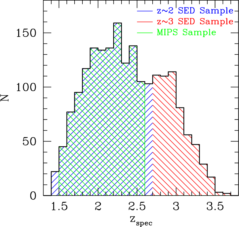
Figure 1.— Spectroscopic redshift distributions of 1959 galaxies at redshifts $1.4\leq z_{\rm spec}\leq 3.7$, color coded according to the subsamples considered (see Table 2).

3. STELLAR POPULATION MODELING: GENERAL PROCEDURE

In this section, we discuss the general procedure used to model the stellar populations of galaxies in our sample. There are a number of assumptions that enter into such modeling, such as the adopted star formation history (e.g., constant, exponentially declining, or rising), the imposition of a lower limit to the age of a galaxy, and the choice of attenuation curve. In the subsequent sections, we discuss and motivate our assumptions by utilizing the multi-wavelength data that exist in a subset of the fields of our survey.

Stellar masses are inferred by modeling the broadband photometry of galaxies, using the full rest-frame UV through near-IR photometry to fit for their stellar populations. For the fitting, we considered only those galaxies that are directly detected at wavelengths longward of rest-frame $4000$ Å  which, for the majority of the sample considered here, includes the F160W, $K_{\rm s}$, and IRAC bands. Further, we excluded from the fitting any AGN that were identified with strong UV emission lines (e.g., Ly$\alpha$, CIV) or had a power law SED through the IRAC bands. Previous efforts to model the stellar populations of galaxies in our sample are described in Shapley et al. (2005), Erb et al. (2006b), Reddy et al. (2006a), and Reddy et al. (2010). The latest solar metallicity models of S. Charlot & G. Bruzual (in preparation, hereafter CB11) that include the Marigo & Girardi (2007) prescription for the thermally-pulsating Asymptotic Giant Branch (TP-AGB) evolution of low- and intermediate-mass stars are used in the fitting. The stellar masses obtained with these newer models are generally lower than those based on the Bruzual & Charlot (2003) models for galaxies with ages $\gtrsim 200$ Myr (Reddy et al., 2010). The relative contribution of the TP-AGB phase is still debated (e.g., Muzzin et al. 2009; Kriek et al. 2010; Melbourne et al. 2012), and we note that adopting the Bruzual & Charlot (2003) models does not significantly alter our results.

If such measurements were available, we corrected the broadband photometry (optical and/or $K_{\rm s}$-band) for the effect of Ly$\alpha$ emission/absorption and/or H$\alpha$ emission. We did not explicitly correct for [OIII] emission, which lies in the $K_{\rm s}$-band at $z\sim 3$ and the F160W band at $z\sim 2$, as [OIII] line measurements were not available. However, neglecting the correction for Ly$\alpha$, H$\alpha$, and/or [OIII] emission for most of the galaxies in our sample results in differences in stellar masses and ages that are substantially smaller than the marginalized errors on ages and stellar masses (Reddy et al., 2010). This is due in part to the inclusion of the IRAC data where line contamination is not an issue, and where such data provide an additional lever arm to measure the strength of the Balmer and $4000$ Å  breaks.

For each galaxy, we considered a CSF model and exponentially declining star formation histories with characteristic timescales $\tau_{\rm d}=$ 10, 20, 50, 100, 200, 500, 1000, 2000, and 5000 Myr. For comparison, we also investigated the effect on the stellar population parameters if we adopt exponentially rising star formation histories, where the SFR, $\Psi$, is expressed as:

$$\Psi(t)\equiv\Psi_{\rm o}{\rm exp}(t/\tau_{\rm r}),$$ (1)

where $\Psi_{\rm o}$ is the normalization factor, $t$ is time (or age), and $\tau_{\rm r}$ is the exponential timescale for the rising history. We have considered exponential timescales $\tau_{\rm r}=100$, 200, 500, 1000, 2000, and 5000 Myr. These star formation histories mimic linearly increasing ones if $t_{\rm age}\ll\tau_{\rm r}$. We further considered a range of ages spaced roughly logarithmically between 50 and 5000 Myr, excluding ages older than the age of the universe at the redshift of each galaxy. The lower age limit of $50$ Myr is adopted to reflect the dynamical timescale as inferred from velocity dispersion and size measurements of $z\sim 2$ LBGs (Erb et al., 2006a; Law et al., 2009, 2012); the imposition of this age limit precludes galaxies from having unrealistic ages that are substantially younger than the dynamical timescale. As discussed below, we also investigate the effect of relaxing this age constraint and show how adopting a lower age limit (combined with a different attenuation curve) can resolve the discrepant SED-inferred SFRs of young galaxies relative to those obtained from direct measurements of the SFRs derived from combining UV and Spitzer/MIPS $24$ $\mu$m data. Finally, reddening is taken into account by employing the Calzetti et al. (2000) attenuation curve (but see below) and allowing $E(B-V)$ to range between 0.0 and 0.6. The choice of the Calzetti model is motivated by the good agreement between the Calzetti dust corrections and those determined from Spitzer/MIPS $24$ $\mu$m and Herschel/PACS $100$ and $160$ $\mu$m inferences of the infrared luminosities (Reddy et al. 2006b, 2010, 2012).

The model SED at each $\tau$ and age ($t_{\rm age}$) combination is reddened, redshifted, and attenuated blueward of rest-frame $1216$ Å  for the opacity of the IGM using the Madau (1995) prescription. The best-fit normalization of this model is determined by minimizing its $\chi^{2}$ with respect to the observed $U_{\rm n}G{\cal R}+JK_{\rm s}$+F160W+IRAC (3.6$-$8.0 $\mu$m) photometry. This normalization then determines the SFR and stellar mass. The model (and normalization) that gives the lowest $\chi^{2}$ is taken to be the best-fit SED. Typically there are several best-fit models that may adequately describe the observed photometry, even when the redshift is fixed to the spectroscopic value, though there is generally less variation in stellar mass than in the other parameters ($\tau$, $t_{\rm age}$, $E(B-V)$) among these best-fit models (Sawicki & Yee, 1998; Papovich et al., 2001; Shapley et al., 2001, 2005). Below, we consider a variety of star formation history models with different assumptions for the age limit and attenuation curve (Table 3).

Table 3Description of SED Models

Model	Assumptions	RMS
Model A	Constant Star Formation	0.44
	Calzetti Attenuation Curve
	No Age Limit
Model B	Declining Star Formation	0.48
	Calzetti Attenuation Curve
	No Age Limit
Model C	Rising Star Formation	0.44
	Calzetti Attenuation Curve
	No Age Limit
Model D	Constant Star Formation	0.44
	Calzetti Attenuation Curve
	$t_{\rm age}>50$ Myr
Model E	Declining Star Formation	0.48
	Calzetti Attenuation Curve
	$t_{\rm age}>50$ Myr
Model F	Rising Star Formation	0.46
	Calzetti Attenuation Curve
	$t_{\rm age}>50$ Myr
Model G	Constant Star Formation	0.46
	Calzetti/SMC Attenuation Curves
	$t_{\rm age}>50$ Myr
Model H	Declining Star Formation	0.50
	Calzetti/SMC Attenuation Curves
	$t_{\rm age}>50$ Myr
Model I	Rising Star Formation	0.48
	Calzetti/SMC Attenuation Curves
	$t_{\rm age}>50$ Myr

4. MULTI-WAVELENGTH CONSTRAINTS ON THE SFRs AND STELLAR POPULATIONS OF HIGH-REDSHIFT GALAXIES

In this section, we compare the SFRs derived from SED fitting (SFR[SED]) with those calculated from combining the UV and MIPS data (SFR[IR+UV]). As discussed in Section 2, there are 302 galaxies in our sample with MIPS $24$ $\mu$m observations and spectroscopic redshifts $1.5\leq z\leq 2.6$ (121 of these galaxies are detected individually at $24$ $\mu$m); it is at these redshifts where the $24$ $\mu$m fluxes are sensitive to the rest-frame 8 $\mu$m emission, which in turn can be converted to $L_{\rm IR}$. Using the procedure described in Reddy et al. (2010), we k-corrected the $24$ $\mu$m fluxes to estimate rest-frame 8 $\mu$m luminosities ($L_{\rm 8}$). We then assumed a ratio $L_{\rm IR}/L_{\rm 8}=8.9\pm 1.3$, as determined from a stacking analysis of the Herschel/PACS 100 and 160 $\mu$m data for a subset of the same galaxies considered here (i.e., those in the GOODS-North field; Reddy et al. 2012). The Kennicutt (1998) relations are then used to convert $L_{\rm IR}$ and $L_{\rm UV}$ (uncorrected for extinction) to SFRs, the sum of which gives the bolometric SFR.

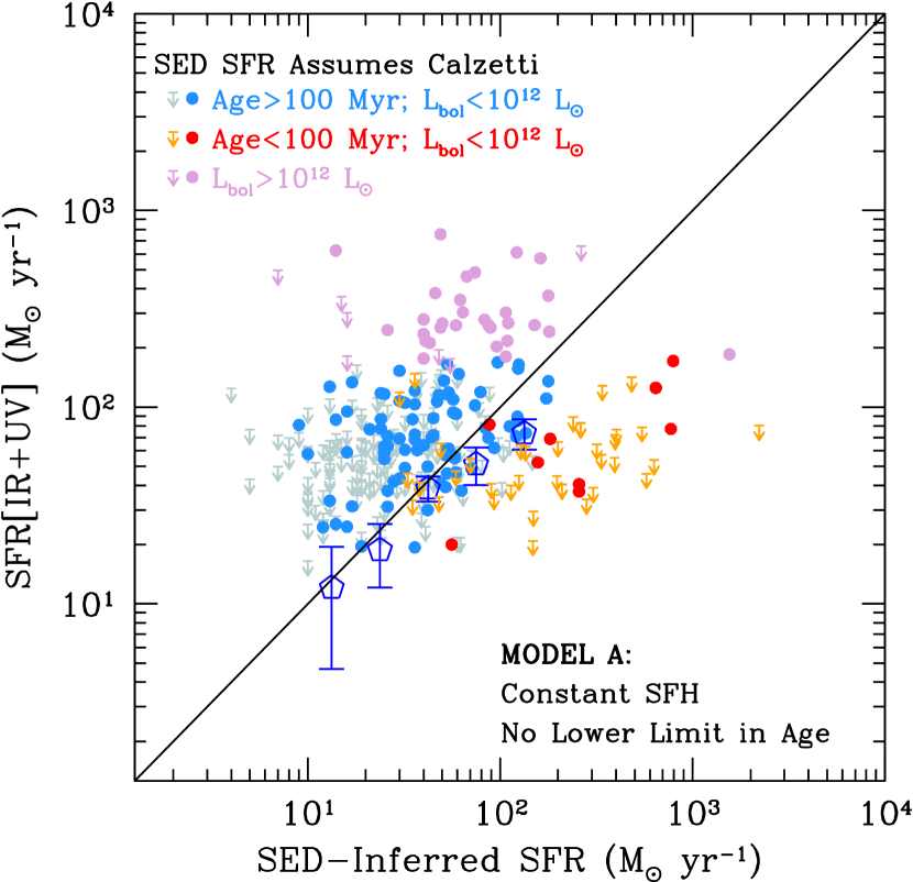
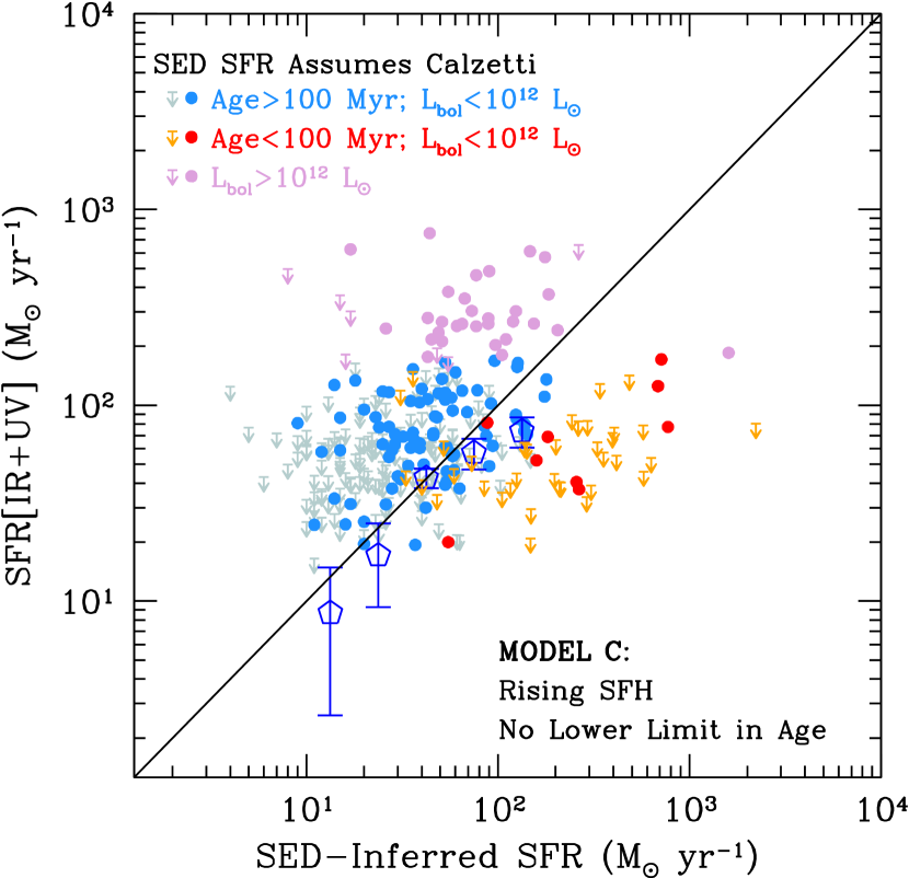
Figure 2.— Comparison between SFRs derived from SED fitting and those computed from combining MIPS $24$ $\mu$m and UV data. Points are color coded to differentiate galaxies with large bolometric luminosities ($L_{\rm bol}>10^{12}$ L_⊙), typical galaxies that form the bulk of the sample ($L_{\rm bol}\leq 10^{12}$ L_⊙ and $t_{\rm age}>100$ Myr), and young galaxies with $t_{\rm age}\leq 100$ Myr. Upper limits are points denote galaxies with $24$ $\mu$m nondetections and detections, respectively. The large pentagons show the average $24$ $\mu$m plus UV determined SFR in bins of SED-inferred SFR for typical galaxies, as determined from a $24$ $\mu$m stacking analysis (see the text). The results for a constant and rising star formation history, with no lower limit imposed on the age, are shown in the left and right panels, respectively.

Note that bolometric SFR computed in this way is not entirely independent of the stellar population because the conversion from $L_{\rm UV}$ to SFR will depend on the star formation history and age. This dependence is discussed in detail in Appendix A. For exponentially declining star formation histories where $t\gg\tau_{\rm d}$, the factor to convert $L_{\rm UV}$ to SFR will be substantially smaller than the Kennicutt (1998) value. More generally, for all of the models considered here (declining, constant, and rising), the conversion factor is at least a factor of two larger than the canonical value for ages $\lesssim 10$ Myr. For convenience, in Appendix A we provide formulae to compute the conversion factor between $L_{\rm UV}$ and SFR for different star formation histories and ages, assuming the CB11 stellar population synthesis models, a Salpeter (1955) IMF between 0.1-100 M_⊙, and solar metallicity. Finally, we note that the factor to convert $L_{\rm IR}$ to SFR is also somewhat dependent on galaxy age, with the Kennicutt (1998) conversion valid for starbursts with ages $\lesssim 100$ Myr. At older ages, there are the competing effects of lower dust opacity and heating from older stellar populations that can modulate the conversion factor between $L_{\rm IR}$ and SFR (Kennicutt, 1998). These effects at older ages are likely to be negligible for most of the high-redshift galaxies studied here due to their larger SFRs, and lower stellar masses, compared to the local galaxies used to calibrate the relationship between $L_{\rm IR}$ and SFR.

For simplicity, we assume the canonical Kennicutt (1998) relations to convert $L_{\rm IR}$ and $L_{\rm UV}$ to SFR, and discuss below how changing the $L_{\rm UV}$-SFR conversion factor affects our results. The MIPS+UV derived SFRs are compared to the SED-inferred SFRs in Figure 2. Below, we discuss in turn the three sets of objects that differentiate themselves in the plane of SFR[IR+UV] versus SFR[SED].

4.1. SFRs of Typical Star-forming Galaxies at $z\sim 2$

This subsection highlights the results found for typical star-forming galaxies, defined as those galaxies with best-fit ages $>100$ Myr and bolometric luminosities $L_{\rm bol}<10^{12}$ L_⊙. Here, $L_{\rm bol}$ is taken as the sum of the UV and IR luminosities, where $L_{\rm IR}$ is computed from the $24$ $\mu$m data using the $L_{\rm IR}/L_{\rm 8}$ ratio discussed above. Because $60\%$ of the galaxies are not detected at $24$ $\mu$m, we have stacked the $24$ $\mu$m data for typical galaxies in bins of SFR[SED] to determine the average bolometric SFR. The stacking procedure is discussed in Reddy et al. (2006b). Uncertainties in the stacked bolometric SFR are computed by combining in quadrature the measurement uncertainty in the mean $24$ $\mu$m flux and the uncertainty in the mean UV luminosity of galaxies contributing to the stack.

SFR[IR+UV] derived in this manner agrees well on average with SFR[SED] assuming constant star formation and no age limit (large pentagons in the left panel of Figure 2). Taking into account upper limits using the ASURV statistical package (Isobe et al., 1986), which includes the expectation maximization (EM) parametric survival estimator for censored data, we compute an rms dispersion about the best-fit linear relation between SFR[IR+UV] and SFR[SED] of 0.44 dex (Table 3). Based on the stacking analysis and the survival analysis, we conclude that there is a good agreement between the MIPS+UV and SED derived SFRs for typical star-forming galaxies at $z\sim 2$. These results are not surprising because previous investigations have shown that on average the Calzetti et al. (2000) corrections for dust obscuration (which are assumed in the SED fitting procedure) reproduce the values estimated from mid and far-infrared, radio, and X-ray data for galaxies at $z\sim 2-3$ (e.g., Nandra et al. 2002; Seibert et al. 2002; Reddy & Steidel 2004; Reddy et al. 2006b; Daddi et al. 2007; Pannella et al. 2009; Reddy et al. 2010; Magdis et al. 2010; Reddy et al. 2012).

4.2. SFRs of Ultraluminous Infrared Galaxies at $z\sim 2$

Turning our attention to ultraluminous infrared galaxies (ULIRGs), we find that those galaxies with $L_{\rm bol}>10^{12}$ L_⊙ have bolometric SFRs that exceed by up to a factor of ten the SFRs[SED]. The $24$ $\mu$m fluxes of the IR-luminous sources in our sample tend to over-predict their $L_{\rm IR}$ by a factor of $\approx 2$, relative to the IR estimates obtained by including far-IR data (e.g., from Herschel; Reddy et al. 2012). Further, as shown in several other investigations, the Calzetti et al. (2000) dust corrections for such objects are typically too low due to the fact that much of the star formation is completely obscured by dust, and hence the UV slope decouples from extinction for such highly obscured galaxies (e.g., Goldader et al. 2002; Reddy et al. 2006b, 2010).

4.3. SFRs of Young Galaxies at $z\sim 2$

A noted problem in stellar population modeling is the distribution of unrealistically young ages derived for non-negligible fractions of galaxies in high-redshift samples, particularly those selected in the rest-UV or rest-optical (Shapley et al., 2001; Maraston et al., 2010). This is commonly referred to as the “outshining” problem, where the SED of a galaxy may be dominated by the youngest stellar population even at near-IR wavelengths, in which case the best-fit models (irrespective of the star formation history) may have very young ($\lesssim 100$ Myr) ages with very large values of SFR and reddening (e.g., Maraston et al. 2010; Wuyts et al. 2011). We have investigated the validity of these young models by cross-checking the SFRs derived using them with those measured directly from MIPS $24$ $\mu$m and UV data.

For such young ($t_{\rm age}<100$ Myr) objects (the third set of objects denoted in Figure 2), we find that SFRs[SED] are systematically larger than SFRs[IR+UV]. This offset cannot be completely accounted for by a change in the conversion between UV luminosity and SFR. In particular, the bulk of these young galaxies have ages (derived with the CSF assumption) as short as $7$ Myr. For these ages, the conversion between UV luminosity and SFR is about a factor of two larger than in the CSF case where $t_{\rm age}>100$ Myr (Appendix A). Given the typical dust attenuation of these “young” galaxies of $L_{\rm IR}/L_{\rm UV}\approx 1$ (e.g., Reddy et al. 2006b, 2012), modifying the UV-SFR conversion upward by a factor of two will increase SFR[IR+UV] by $50\%$, or $0.18$ dex. This difference is not sufficient to account for the offset between SFR[SED] and SFR[IR+UV] for the young subsample.

Galaxies at $z\sim 2$ that are identified as being young based on their CSF model fits have UV slopes, $\beta$, which are on average redder than the slopes of older galaxies at the same redshifts, with a difference in $\beta$ of $\langle\delta\beta\rangle\simeq 0.3$ (Figure 3). If we assume that a Calzetti attenuation curve applies for such galaxies, then we would find them to be more dust obscured, given their redder $\beta$, and hence to have larger bolometric SFRs, than the “typical” galaxies discussed above. Clearly, the very large dust obscuration and bolometric SFRs inferred for such galaxies cannot be correct, based on the comparison of these SFRs with those derived directly from combining the MIPS and UV data (Figure 2).

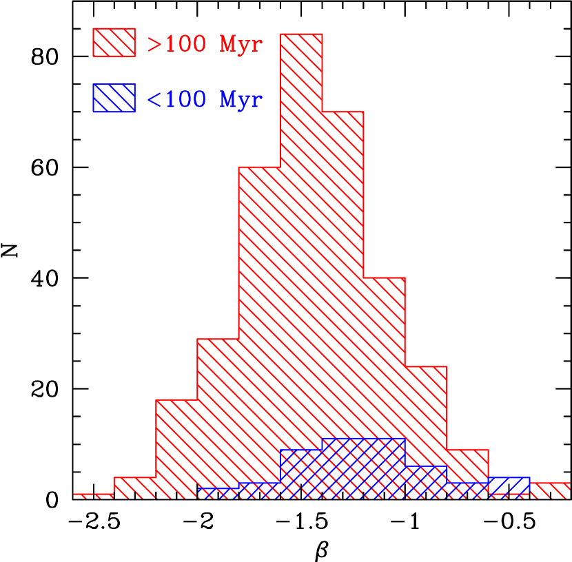
Figure 3.— $\beta$ distribution for galaxies with Calzetti-derived ages $>100$ Myr (red histogram) compared to that of galaxies with Calzetti-derived ages $<100$ Myr (blue histogram), in the sample of 392 UV selected galaxies of Reddy et al. (2010). The ages assume a CSF model. A two-sided K-S test indicates a probability $P\lesssim 0.01$ that the two distributions are drawn from the same parent sample. On average, the younger galaxies have UV slopes that are $\langle\delta\beta\rangle\simeq 0.3$ redder than those of older galaxies.

4.4. Results for Other Star Formation Histories

We conclude this discussion by noting that the assumption of exponentially rising star formation histories results in the same qualitative behavior for the three sets of galaxies discussed above (typical galaxies, ULIRGs, and young galaxies; Figure 2). The RMS around the best-fit relation between SFR[SED] and SFR[IR+UV] is listed in Table 3. In contrast, the assumption of exponentially declining star formation histories results in SFRs[SED] for typical galaxies that lie systematically below SFRs[IR+UV] (Figure 4). A similar conclusion is reached when comparing dust-corrected H$\alpha$ estimates of the SFR with those computed from fitting exponentially declining models to the broadband photometry of a subset of galaxies in our sample (Erb et al., 2006a).

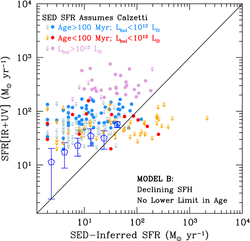
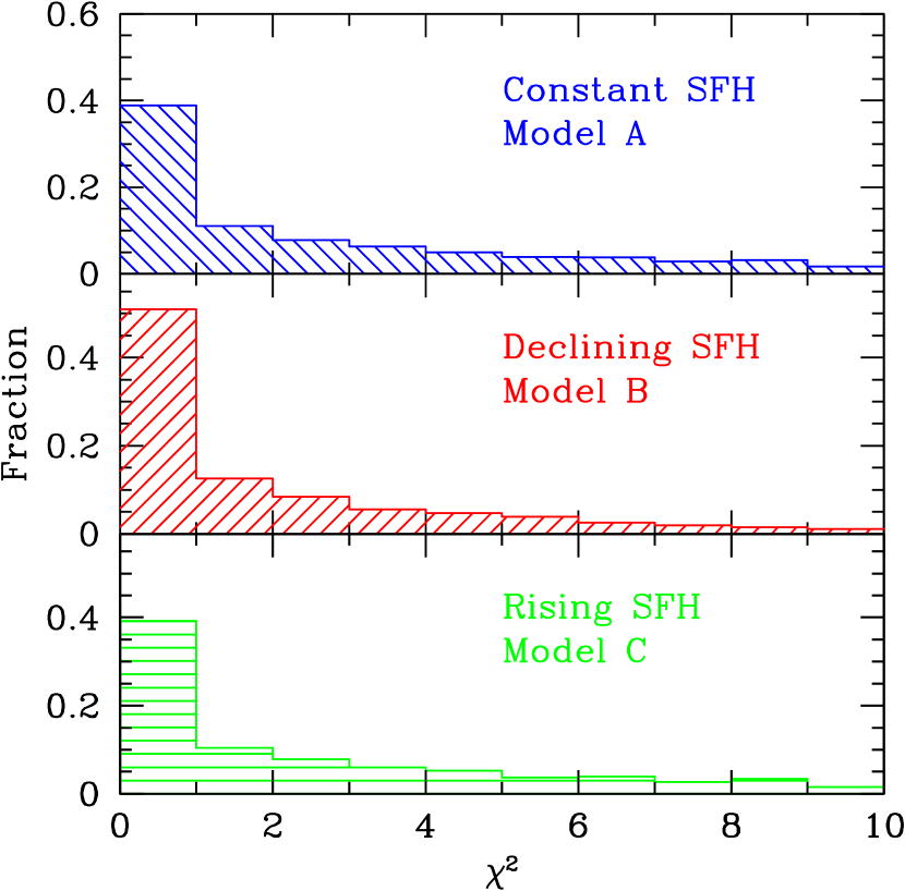
Figure 4.— (Left:) Same as Figure 2, where we have assumed the best-fit exponentially declining star formation history. (Right:) Histograms of the $\chi^{2}$ distributions of the best-fit SED models to the broadband photometry for 1959 galaxies with spectroscopic redshifts $1.4\leq z\leq 3.7$, assuming declining, constant, and rising star formation histories (corresponding to Models A, B, and C, respectively, as listed in Table 3). The histograms have been normalized to the total number of galaxies (1959).

The discrepancies that arise from adopting an exponentially declining star formation history stem from two effects. The first is that the redness of the UV continuum is, to a greater extent, attributed to older stars in the case when $t_{\rm age}/\tau_{\rm d}>1$, relative to the CSF case. Hence, the $E(B-V)$ for declining models will on average be lower, implying lower SFRs. The second effect is that the ratio of the SFR to UV continuum is generally lower for galaxies with smaller $\tau_{\rm d}$ (Appendix A; see also Shapley et al. 2005 for a discussion of these points), which also results in smaller SFRs for a given UV luminosity. Shapley et al. (2005) discuss other reasons why extreme declining star formation histories where $\tau_{\rm d}<100$ Myr and $t_{\rm age}/\tau_{\rm d}\gg 1$ are implausible for the vast majority of galaxies in our sample. In particular, the correspondence between the H$\alpha$ and UV derived SFRs for $z\sim 2$ galaxies (Erb et al., 2006a; Reddy et al., 2010), as well as the presence of O star features in the UV spectra of galaxies in our sample—e.g., Ly$\alpha$ emission, and Wolf Rayet signatures including broad HeII 1640 Å  and P-Cygni wind features in the CIV and SiIV lines (Shapley et al., 2003; Quider et al., 2009)—imply that the UV continuum is likely dominated by O stars, contrary to the expectation if $t_{\rm age}/\tau_{\rm d}\gg 1$.

The importance of the comparison to the MIPS+UV SFRs is underscored by the fact that one cannot discriminate between these various star formation histories, even the simple ones considered here, from the broadband SEDs alone. As the right panel of Figure 4 shows, the $\chi^{2}$ distributions of the best-fit SEDs for the different star formation histories are roughly similar. The MIPS data allow us to break this impasse, and they can be used to demonstrate clearly that, on average, the exponentially declining models yield SFRs that are statistically inconsistent with those obtained from direct measures of the SFRs. Given this finding, we focus the subsequent discussion on constant and rising star formation histories.

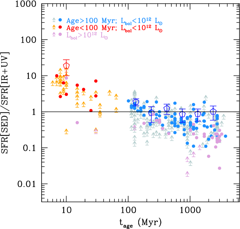
Figure 5.— Ratio of SED-inferred SFR and SFR derived from combining MIPS and UV data, vs. stellar population age, for Model C (Table 3; rising star formation history with no age limit). Symbols are the same as in Figure 2. The large red pentagon denotes the median value based on stacking the $24$ $\mu$m data for the galaxies with $t_{\rm age}<100$ Myr. For Model C, the SED-inferred SFRs of the young galaxies exceed by an order of magnitude those estimates from combining the MIPS and UV data.

5. RESOLVING THE CONFLICTING SFRs FOR YOUNG GALAXIES

As noted in Section 4.3, all of the star formation histories considered here predict SFRs that are substantially larger than those computed from the MIPS and UV data for young galaxies with $t_{\rm age}<100$ Myr. Figure 5 shows that this systematic difference is a strong function of age, being most severe for galaxies with $t_{\rm age}\lesssim 50$ Myr. Given that the true ages are unlikely to be significantly smaller than the dynamical timescale of $\simeq 50$ Myr, we have imposed the restriction $t_{\rm age}>t_{\rm dyn}\simeq 50$ Myr when fitting the SEDs. Note that the exact limit in age is unimportant given the relatively few galaxies with $20\lesssim t_{\rm age}\lesssim 100$ Myr. Adopting an age restriction, the comparison between SED and MIPS+UV SFRs is shown in Figure 6. At face value, based on the individual data points, the agreement between the SFRs for galaxies with $t_{\rm age}<100$ Myr is better once we have restricted the age to be older than $t_{\rm age}=50$ Myr. However, a MIPS stack for those galaxies with $50<t_{\rm age}<100$ Myr results in a formal non-detection at $24$ $\mu$m, inconsistent at the $3\sigma$ level with our expectation based on the SFRs[SED] for these galaxies (red pentagons in Figure 6).

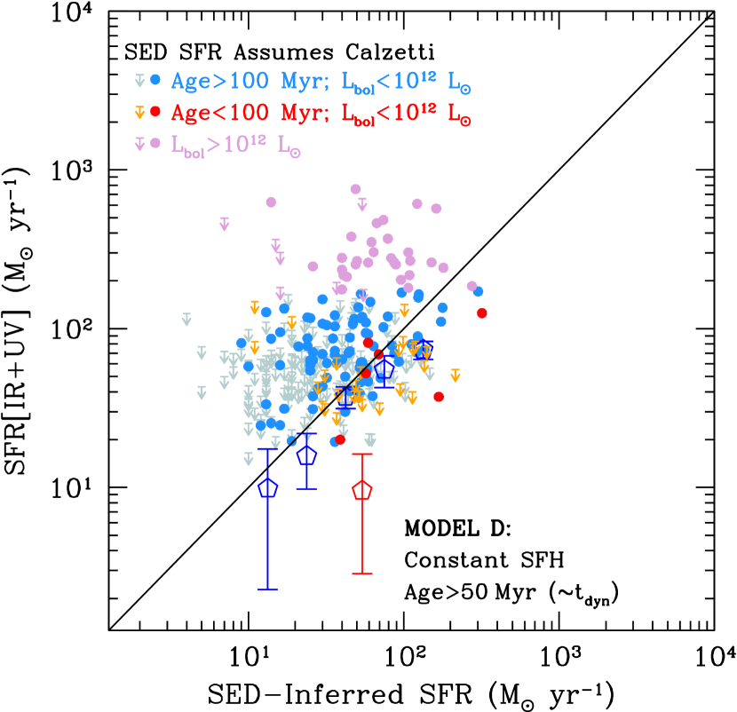
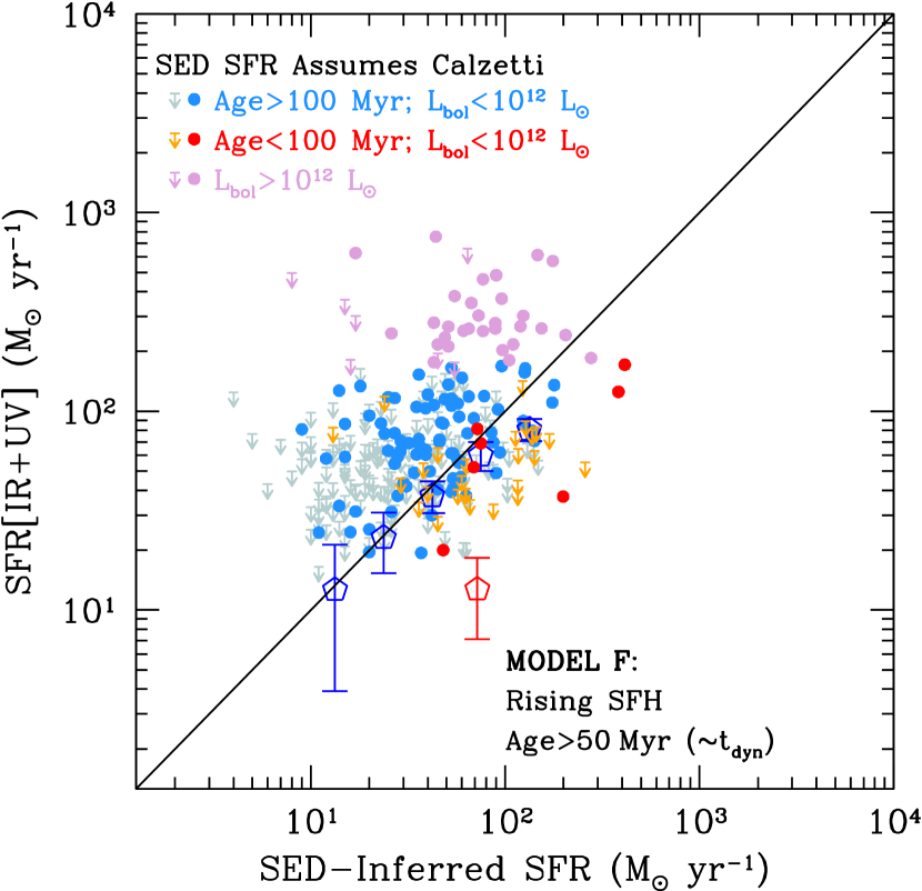
Figure 6.— Same as Figure 2 where we have imposed a lower limit on the age of $t_{\rm age}=50$ Myr in the SED modeling including constant (left) and rising (right) star formation histories. The large red pentagon denotes the stacked results for galaxies with $50\leq t_{\rm age}<100$ Myr.

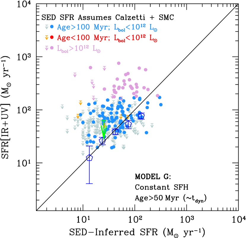
Figure 7.— Same as Figure 6 where we have imposed a lower limit on the age of $t_{\rm age}=50$ Myr in the SED modeling, and we have remodeled those galaxies with Calzetti inferred ages $t_{\rm age}<100$ Myr with an SMC attenuation curve. Results are shown for the constant (left) and rising (right) star formation histories. The green arrow in the left panel indicates the 3 $\sigma$ upper limit to SFR[IR+UV] for the 4 $24$ $\mu$m undetected galaxies that are considered young under the assumption of the SMC attenuation curve.

5.1. Age Dependence of the UV Attenuation Curve

One possible solution to this discrepancy comes from the correlation between the dust obscuration, $L_{\rm IR}/L_{\rm UV}$, and UV slope ($\beta$) for these young galaxies. In particular, Reddy et al. (2006b, 2010) found that such galaxies have redder UV slopes for a given dust attenuation relative to older galaxies with $t_{\rm age}>100$ Myr. This effect may stem from a geometrically different distribution of dust with respect to the stars in a galaxy where, for young galaxies, this dust may preferentially lie foreground to the stars. Regardless, the attenuation curve obtained for the young galaxies (on average) appears to mimic that of the Small Magellanic Cloud (SMC) attenuation curve. A steeper attenuation curve (e.g., SMC curve) will result in older ages than those obtained in the Calzetti case; because not as much dust is needed to redden the continuum for a foreground screen of dust relative to a uniform distribution of dust and stars, the redness of the UV slope will be attributed more to an older stellar population than dust attenuation. If we remodel those galaxies with Calzetti-inferred ages $50<t_{\rm age}<100$ Myr with the SMC attenuation curve, then the fraction of galaxies that are still considered to be “young” ($t_{\rm age}<100$ Myr) is reduced by at least a factor of nine. In the CSF case, the number of galaxies with $t_{\rm age}<100$ Myr drops from 36 to just 4. In the exponentially rising case, this number drops from 36 to just 2. The small fraction of galaxies that are still considered young under the SMC assumption have upper limits in SFR[IR+UV] that are consistent with SFR[SED] when we assume an SMC attenuation curve (Figure 7). Hence, if we assume an SMC attenuation curve, there is no longer a conflict between the upper limit to SFR[IR+UV] (from the MIPS-nondetection) and SFR[SED] for the young galaxies.

At first glance, the adoption of a lower limit in age that is equivalent to the dynamical timescale, combined with a different attenuation curve for the “young” galaxies, may appear to be a contrived and inelegant solution to resolving the discrepancy between SFR[IR+UV] and SFR[SED] for such galaxies. However, our primary goal is to derive SED parameters that are based on physically motivated ages (i.e., dynamical time constraints) and are consistent with observations of the dustiness and UV slopes for such galaxies (Reddy et al., 2006b, 2010). A consistent treatment of the multi-wavelength data allows us to resolve the discrepancy between the different measures of SFRs for young galaxies.

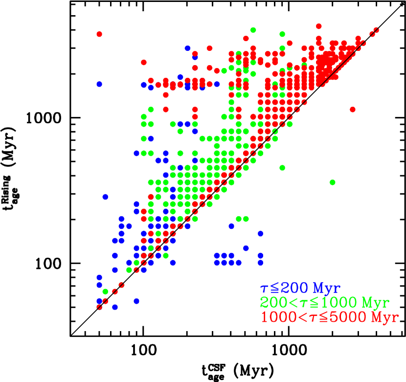
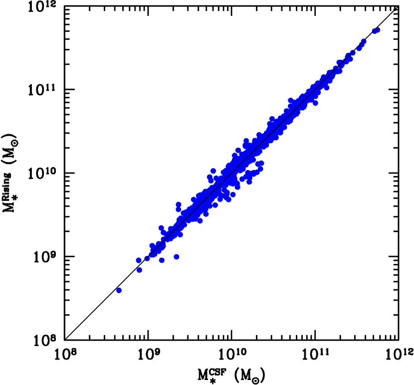
Figure 8.— Comparison of the ages (left) and stellar masses (right) between the constant (Model G) and rising star formation models (Model I), respectively.

5.2. Summary of SFR Comparisons

In the previous sections, we presented the comparison of the SFRs determined from independent indicators of dust (MIPS $24$ $\mu$m) to those computed from fitting the broadband SEDs of galaxies at redshifts $1.5\lesssim z\lesssim 2.6$. Three sets of galaxies are identified in this comparison: (1) ULIRGs with $L_{\rm bol}\approx L_{\rm IR}>10^{12}$ L_⊙; (2) typical star-forming galaxies with $L_{\rm bol}\leq 10^{12}$ L_⊙ and ages $t_{\rm age}\gtrsim 100$ Myr; and (3) “young” galaxies with $L_{\rm bol}\leq 10^{12}$ L_⊙ and ages $t_{\rm age}\lesssim 100$ Myr. For typical galaxies, an exponentially declining star formation history yields SFRs that are inconsistent with those obtained from combining the MIPS and UV data. Assuming constant or rising star formation histories yields SFRs that are in reasonable agreement with the MIPS+UV determinations. Alternatively, none of the simple star formation histories considered here (constant, declining, or rising) are able to reproduce the lower SFRs found for “young” galaxies. We explore several possibilities for resolving this discrepancy, including dynamical time constraints and systematics in the UV attenuation curve. A physically plausible solution — and one which is consistent with independent measurements of the age dependence of the dust attenuation curve at $z\sim 2-3$ (Reddy et al., 2006b, 2010) — is to adopt a lower limit in age corresponding to the dynamical timescale typical of galaxies in our sample ($\simeq 50$ Myr), and to assume a steeper (e.g., “SMC”) attenuation curve for the young galaxies (corresponding to Models G and I in Table 3). Based on these findings, we proceed in the next section with a discussion of the stellar masses and ages derived from constant and rising star formation histories.

6. INTERDEPENDENCIES OF THE SED PARAMETERS

Having just discussed the most plausible star formation histories that are constrainable with the available data, in this section we focus on the systematic variations in age and stellar mass with the overall form of the star formation history (constant versus rising), the typical uncertainties in ages and stellar masses, and the correlation between SFR and stellar mass.

6.1. Systematic Variations in Age and Stellar Mass

The ages and stellar masses derived for 1959 objects with spectroscopic redshifts $1.4\leq z\leq 3.7$, assuming constant and exponentially rising star formation histories, are shown in Figure 8. Histograms of the age and stellar mass distributions are presented in Figure 9. The stellar mass for any given galaxy derived with a rising star formation history is essentially identical within the uncertainties (that stem primarily from photometric errors and the degeneracy between the parameters being fit) to those obtained with a CSF history. The primary difference, therefore, is in the distribution of best-fit ages; ages derived with a rising star formation history are older by $\approx.12$ dex. The fraction of galaxies in our spectroscopic sample with derived ages older than 1 Gyr increases from $20\%$ to $32\%$ when we assume rising star formation histories versus CSF.

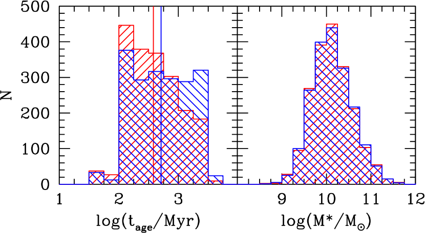
Figure 9.— Histograms of age and stellar mass for the constant (red) and rising (blue) star formation histories. The vertical lines in the left panel indicate the mean age found when assuming the constant and rising star formation histories.

We can better understand these trends by examining the evolution in the stellar mass-to-light ratio ($M/L$) as a function of galaxy age for the different star formation histories considered here. At early times, for ages $t_{\rm age}\lesssim\tau_{\rm r}$, the light is dominated by current star formation and the $M/L$ ratio is low. As the stellar mass builds up, older stars will begin to contribute significantly to the light, causing the $M/L$ ratio to increase. Neglecting dust reddening, for $t_{\rm age}\gg\tau_{\rm r}$, the $M/L$ ratio stabilizes to some constant value. In reality, the $M/L$ ratio will still increase (even though the ratio of stellar mass to total SFR may remain roughly constant), because dust reddening will increase with SFR, and hence the bolometric light will suffer an increasing amount of obscuration (Figure 10).

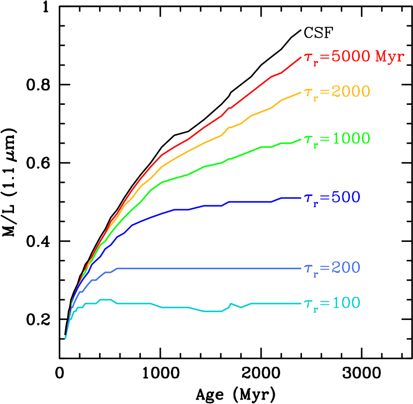
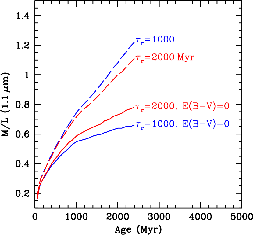
Figure 10.— Left: Stellar mass to light ratio at $1.1$ $\mu$m (in solar units) as a function of age for CSF and exponentially rising star formation histories, with $\tau_{r}=100$ to $5000$ Myr. The curves assume $E(B-V)=0$. Right: Evolution in $M/L$ ratio including the effects of dust attenuation (dashed lines), where we have assumed the relationship between SFR and $E(B-V)$ as determined from the SED modeling, compared to the cases with no dust attenuation, $E(B-V)=0$ (solid lines). For this example, we consider $\tau_{\rm r}=1000$ and $2000$ Myr, and an initial SFR of $20$ M_⊙ yr^-1. The difference between the curves for $\tau_{\rm r}=1000$ Myr is larger than the difference between the $\tau_{\rm r}=2000$ Myr curves because the SFR, and hence dust reddening, rises more rapidly for smaller values of $\tau_{\rm r}$.

Regardless, as shown in Figure 10, the $M/L$ ratio (at rest-frame $1.1$ $\mu$m, corresponding roughly to an observed wavelength at $z\sim 2.3$ that coincides with IRAC channel 1) increases more slowly with age for galaxies with smaller values of $\tau_{\rm r}$. Hence, for the same $M/L$ ratio, rising star formation histories correspond to an older age than a CSF history. Note that these trends hold on average, and there is still a fair fraction of galaxies where the ages (and stellar masses) do not change substantially between the CSF and rising star formation histories. In particular, approximately $55\%$ of galaxies in our sample have a best-fit $\tau_{\rm r}=5000$ Myr, and it is for these longer exponential timescales that the $M/L$ ratio is not substantially different than that obtained in the CSF case when $t_{\rm age}<\tau_{\rm r}$. In any case, the stellar mass distributions do not change substantially when we adopt a rising versus CSF history, and in both cases, the mean stellar mass of galaxies in our spectroscopically confirmed (${\cal R}<25.5$) sample at $z\sim 2.3$ is $\langle M_{\ast}\rangle=1.6\times 10^{10}$ M_⊙. As we discuss in Section 7.2.1, the mean stellar mass is a strong function of absolute magnitude, and including galaxies fainter than our spectroscopic limit will result in a lower mean stellar mass.

6.2. The “Ages” of Galaxies with Rising Star Formation Histories

As just discussed, rising star formation histories require older ages than CSF histories to achieve a given mass-to-light ratio. In general, the ages derived with either a constant or rising star formation history will be a lower limit to the true age, because of the possibility that there may be an underlying older stellar population whose near-IR light is overwhelmed by the near-IR light from current star formation (i.e., the “outshining” problem as discussed above). A further systematic effect pertains to “ages” derived under the assumption of different star formation histories. In the simplest case for constant star formation, the age is simply determined by the time required to build up the observed stellar mass given the current rate of star formation. Integrating Equation 1 yields the stellar mass after time $t$ for an exponentially rising star formation history:

$$M_{\ast}(t)=\Psi_{o}\tau_{\rm r}[{\rm exp}(t/\tau_{\rm r})-1].$$ (2)

For simplicity, we have ignored the gas recycling fraction (i.e., the fraction of gas released back into the interstellar medium (ISM) from supernovae and stellar winds), as adopting this correction will simply adjust downwards the stellar mass by some multiplicative factor close to $\approx 0.7$ (Bruzual & Charlot, 2003). With this parameterization, the stellar mass $M_{\ast}=0$ M_⊙ at time $t=0$. In this case, the “age” is well defined in a mathematical sense, and these are the ages that we have referred to in the previous sections. Note that the specific SFR

$$\phi(t)\equiv\frac{\Psi(t)}{M_{\ast}(t)}=\frac{{\rm exp}(t/\tau_{\rm r})}{\tau_{\rm r}[{\rm exp}(t/\tau_{\rm r})-1]},$$ (3)

is roughly constant as a function of time if $\exp(t/\tau_{\rm r})\gg 1$. As long as this condition is satisfied, the age $t$ can be arbitrarily old. In that case, we would simply adjust the normalization $\Psi_{\rm o}$ for a given $t$ in order to recover the observed stellar mass. As a simple example, if we assume that $\tau_{\rm r}\approx 400$ Myr and we consider ages of $t=1$ and $2$ Gyr, then we must set $\Psi_{\rm o}\approx 3.6$ and $0.3$ M_⊙ yr^-1, respectively, in order for the current stellar mass to be $M_{\ast}\approx 1.6\times 10^{10}$ M_⊙. Given the ambiguity of the derived “age” for a rising star formation history, it is useful to define a characteristic timescale $t_{\rm c}$ over which the galaxy has doubled its stellar mass:

$$t_{\rm c}\equiv t_{\rm age}-t_{\rm 1/2}\approx\tau_{\rm r}\ln(2)=\frac{1}{\phi}\ln(2),$$ (4)

where $t_{\rm 1/2}$ indicates the time at which the galaxy had half of its current stellar mass. We show the comparison between $t_{\rm c}$ and $t_{\rm age}/2$ for the rising and constant star formation models, respectively, in Figure 11. The comparison shows that there is a better correspondence between the times required to double the stellar mass to the currently observed value with a rising and CSF models. Of course, for a given currently observed SFR, the rising history (as compared to a CSF model) will implies a longer amount of time to build up the current stellar mass given that the SFR was lower in the past. In Section 8, we discuss the mass doubling time, derived ages, and implied formation redshifts, in the context of direct observations of $z\gtrsim 3$ galaxies.

Figure 11.— Comparison between the characteristic timescales required to double the stellar mass to the present value with a rising ($t_{\rm c}^{Rising}$) and constant ($t_{\rm age}^{CSF}/2$) star formation histories for the full SED sample of 1959 galaxies.

6.3. Uncertainties in Age and Stellar Mass with Simple Star Formation Histories

As just discussed, the assumption of rising versus CSF histories results in systematic differences in the stellar population ages. Other systematics affecting ages and stellar masses include uncertainties in the IMF, differences between stellar population synthesis models (e.g., Bruzual & Charlot 2003; Maraston et al. 2006; CB11), and the degree to which simple star formation histories can capture the complexity of the “real” star formation history of a galaxy (e.g., Papovich et al. 2001; Shapley et al. 2001, 2005; Marchesini et al. 2009; Muzzin et al. 2009; Maraston et al. 2010; Papovich et al. 2011). While the uncertainties in the complexity of the star formation history of any individual galaxy may be large, if such variations are stochastic (e.g., such as having multiple independent bursts of star formation), then large galaxy samples can be used to average over these stochastic effects and yield insight into the characteristic, or typical, star formation history. In addition to these systematic effects, there are also uncertainties related to our ability to accurately constrain the stellar population model given the flux errors and limited wavelength coverage of photometry. These effects result in typical fractional uncertainties of $\sigma_{\rm age}/\langle t_{\rm age}\rangle=0.5$ and $\sigma_{\rm M^{\ast}}/\langle M^{\ast}\rangle=0.4$, respectively, as determined from Monte Carlo simulations (Shapley et al., 2005; Erb et al., 2006b).

6.4. Relationship between Star Formation Rate and Stellar Mass

The relationship between SFR[IR+UV] and stellar mass for the 302 galaxies at $1.5\leq z_{\rm spec}\leq 2.6$ with MIPS $24$ $\mu$m observations (121 of which are detected at $24$ $\mu$m) is shown in the left panel of Figure 12. Rising star formation histories are assumed; stellar masses derived from a CSF history will be similar. As found by several previous investigations at similar redshifts (e.g., Reddy et al. 2006b; Papovich et al. 2006; Daddi et al. 2007), we find a relatively tight positive correlation between SFR and stellar mass (though we discuss below potential biases), which has typically been interpreted as an indication that most of the stellar mass at these redshifts accumulated in a relatively “smooth” manner and not in major mergers. Taking into account the upper limits with a survival analysis, we find an rms scatter about the best-fit linear relation between the log of SFR and log of stellar mass of $\approx 0.37$ dex, and a slope of $0.97\pm 0.05$.

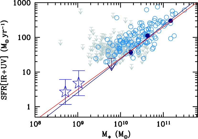
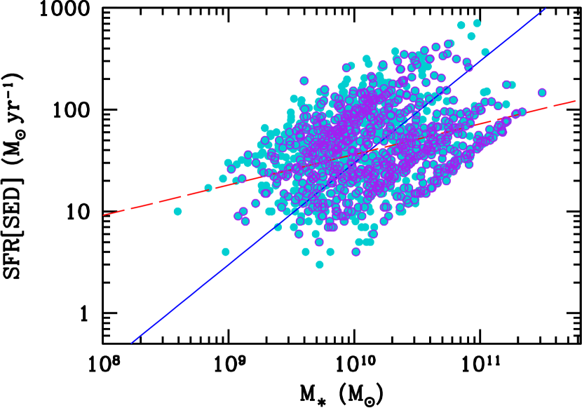
Figure 12.— Left: Relationship between SFR, determined from combining MIPS and UV data, and stellar mass as determined from SED fitting for 302 spectroscopically confirmed galaxies at $1.5\leq z\leq 2.6$. We have assumed rising star formation histories to derive the stellar masses (e.g., using Model I [Table 3]). Upper limits and detections are indicated by the arrows and hollow circles, respectively, and the darker filled symbols and upper limit denote the stacked SFR in bins of stellar mass. The best-fit linear correlation between SFR and M_∗ for the spectroscopic sample, taking into account upper limits, is shown by the solid blue line. The large open stars are for photometrically selected faint $z\sim 2$ galaxies. The red line indicates the relationship found by Daddi et al. (2007) at similar redshifts. Right: Same as left panel, where SFRs are determined from SED fitting of a larger sample of 1264 galaxies with spectroscopic redshifts in the same range as the MIPS sample (cyan points). The purple points show the distribution for the subset of 705 galaxies that have at least two detections longward of the Balmer/4000 Å  breaks. The solid line shows the intrinsic correlation between SFR and $M_{\ast}$, and the dashed line indicates a linear least squares fit to the data.

Because the relationship between SFR and stellar mass has been studied extensively over a large range of redshifts (e.g., Brinchmann et al. 2004; Reddy et al. 2006b; Noeske et al. 2007; Daddi et al. 2007; Stark et al. 2009; González et al. 2010; Sawicki 2011), it is useful to examine how sample selection may bias the measurement of this relationship. The right panel of Figure 12 shows the correlation between SFR and $M_{\ast}$, where SFR is determined solely from the SED fitting (using Model I), for a larger sample of 1244 galaxies with spectroscopic redshifts in the same range as the MIPS sample. For comparison, the distribution of SFR versus stellar mass for the subset of 705 galaxies with at least two detections longward of the Balmer and $4000$ Å  breaks is also shown. We note that the distribution for this subset is similar to that of the larger sample, implying that the inclusion of galaxies with just a single point longward of the Balmer and $4000$ Å  breaks does not systematically bias the distribution of SFR versus $M_{\ast}$. In the SED fitting procedure, both the SFR and stellar mass are determined by the normalization of the model SED to the observed photometry (Section 3). As such, SFR[SED] and $M_{\ast}$ are highly correlated and exhibit an intrinsic slope of unity. However, a linear least squares fit to the data imply a much shallower slope of $0.30$. This bias is a result of the fact that our sample is selected based on UV luminosity (e.g., and not stellar mass). Hence, there will be a Malmquist bias of selecting galaxies with larger SFRs at a given stellar mass for the lowest stellar mass galaxies in our sample. This bias is quantified via simulations that are presented in Appendix B. The effect of this bias on the best-fit relation between stellar mass and near-IR magnitude is discussed in Appendix C. Finally, Appendix E examines the effect of these biases on the determination of mean stellar mass from a UV selected sample.

A comparison of the left and right panels of Figure 12 shows that the Malmquist bias is much less noticeable when the SFR is determined independently of the stellar mass (which is not the case when fitting the SEDs with stellar population models), primarily because the SFRs[IR+UV] have additional scatter associated with them (related to the dispersion in dust extinction at a given UV luminosity) that is decoupled from the method we used to infer $M_{\ast}$ from the SED fitting. As we discuss below, the near-unity slope of the SFR-$M_{\ast}$ relation, where SFRs are determined from the MIPS+UV data, appears to hold to lower stellar masses, and it implies that the specific SFR depends only weakly on stellar mass. We will return to the implication of this result in Section 8.

Before proceeding, we comment briefly on a potential bias that may exist at the bright, high-mass end of the SFR-$M_{\ast}$ relation. As noted in Section 4, the Reddy et al. (2010) conversion between rest-frame $8$ $\mu$m and total IR luminosity reproduces the average $L_{\rm IR}$ computed using stacked Herschel/PACS 100 and $160$ $\mu$m data (Reddy et al., 2012). This conversion is also shown to over-predict $L_{\rm IR}$ for the most bolometrically luminous galaxies in our sample. Correcting for this effect will lower SFR[IR+UV] by up to a factor of two, resulting in a shallower slope of SFR-M_∗ at these high stellar masses where $M_{\ast}\gtrsim 10^{11}$ M_⊙. On the other hand, at a given high stellar mass, our UV selected sample will be biased against the dustiest and hence most heavily star-forming galaxies. This is due the fact that such dusty galaxies either (a) have UV colors that are too red to satisfy the color criteria or (b) are too faint to be represented in the spectroscopic sample (e.g., Reddy et al. 2008, 2010). Inclusion of these missing dusty galaxies would have the opposite effect of steepening the slope of the SFR-M_∗ relation at high stellar masses. Regardless of these two competing biases at the high stellar mass end, correcting for them is unlikely to alter significantly the overall slope of the SFR-M_∗ relation, given that such high SFR galaxies constitute only a small fraction of the number density of $L^{\ast}$ and fainter galaxies (e.g., Reddy et al. 2008; Reddy & Steidel 2009; Magnelli et al. 2011).

6.5. Summary of Age and Stellar Mass Distributions, and SFR-$M_{\ast}$ Relation

Modeling the broadband photometry of spectroscopically confirmed galaxies in the $z\sim 2-3$ sample allows us to examine the distribution of ages and stellar masses. We have shown that rising star formation histories generally yield older ages for a given mass to light ratio relative to the ages obtained with a CSF history. More generally, the “age” of galaxy is not well-defined for a rising star formation history, in the sense that the age can be varied simultaneously with the normalization of the star formation history to yield the same value of current SFR and stellar mass, as long as $\exp(t\tau)\gg 1$. Using SFRs that are derived independently of the stellar masses, we find an intrinsic SFR versus stellar mass correlation with roughly unity slope at $z\sim 2$. So far, we have concerned ourselves with the SED sample which, by construction, only includes those galaxies that had at least one detection longward of the $4000$ Å  break. However, there exist substantial numbers of UV-selected galaxies that are not represented in the SED sample because they are undetected longward of the break. More generally, we expect the SED sample to be biased to galaxies with larger stellar masses at a given SFR relative to the UV sample as a whole. In the next section, we explore this bias by stacking the longer wavelength data for galaxies in our sample, and we also extend the results on the SFR-$M_{\ast}$ relation to UV faint galaxies at the same redshifts.

Table 4Mass to Light Ratios

Rest-frame $\lambda$
($\mu$m)	$N$	Spearman’s $\sigma$	RMS	($\frac{M}{L}$)min	($\frac{M}{L}$)max
$0.50$	98	5.5	0.33	0.07	4.4
$0.67$	491	14.5	0.32	0.06	4.4
$1.1$	643	22.3	0.20	0.14	4.4
$1.4$	673	23.0	0.18	0.18	4.4
$1.8$	180	11.8	0.19	0.24	2.4
$2.4$	190	10.9	0.23	0.21	4.4

7. MASS-TO-LIGHT RATIOS OF $z\sim 2-3$ GALAXIES

7.1. Rest-frame Near-IR $M/L$ Ratios

Because the data required to model the stellar populations do not exist for every galaxy in our sample (e.g., those galaxies that did not have near-IR or IRAC coverage, as well as those undetected at these longer wavelengths), it is useful to establish some empirical relationship between the luminosity of a galaxy and its stellar mass. Given the stellar mass to light ratio ($M/L$), we can then estimate the stellar mass of galaxy based simply on the flux at a given wavelength. The relation between stellar mass and rest-frame near-IR light as probed by the IRAC observations is shown in Figure 13. We have also computed these relations at rest-frame optical wavelengths using the F160W and $K_{\rm s}$-band data As summarized in Table 4, the dispersions between the rest-frame near-IR luminosities and stellar masses are lower than those found between rest-frame optical luminosity and stellar mass, but we note the large variation in mass-to-light ratio even at rest-frame wavelengths where the stellar emission peaks, around $1.6$ $\mu$m. The current star formation in a galaxy may outshine the light from the older stars at rest-frame optical and near-IR wavelengths. In these cases, the ages (and masses) typically reflect those of the current star formation episode, though two component models can be used to determine an upper limit to the hidden stellar mass in such galaxies (e.g., Shapley et al. 2005). For the subsequent discussion, we focus on results using the IRAC $3.6$ $\mu$m data, noting that our results (e.g., derived stellar masses) do not change substantially when we use data from the other IRAC channels.

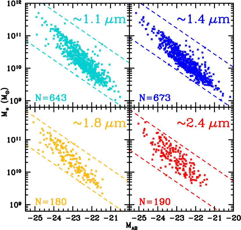
Figure 13.— Relationship between stellar mass and absolute magnitude measured in the four IRAC channels. Approximate rest-frame wavelengths are indicated in each panel, along with the number of objects used to define the relationship. Short dashed lines indicate the minimum and maximum $M/L$ ratio.

Note that there is a systematic trend towards lower $M/L$ at lower stellar mass or fainter near-IR luminosity; i.e., the best-fit relation between near-IR luminosity and stellar mass does not fall onto a line of constant $M/L$. At face value, this systematic trend implies that galaxies with lower stellar masses have larger specific SFRs ($\phi$), resulting in lower $M/L$ ratios. However, as discussed in Section 6.4 and Appendix B, there is Malmquist bias of selecting galaxies with larger SFRs, and hence larger $\phi$, for the lowest mass galaxies in our spectroscopic sample. This directly affects the best-fit relation between stellar mass and near-IR luminosity, as discussed in Appendix C. The basic conclusion from these different best-fit relations is that there are sufficient biases induced by Malmquist effects and not correcting for dust extinction that can produce an erroneously strong trend between $M/L$ ratio and luminosity. For the subsequent discussion, we employ the relations discussed in Appendix C to convert the average near-IR magnitude to stellar mass for galaxies of a given UV luminosity.

7.2. Rest-frame UV Mass-to-light Ratio

The scatter in the $M/L$ ratio increases towards shorter wavelengths, as the current star formation dominates the emission. This can already be seen in the larger scatter in $M/L$ at optical wavelengths relative to that found in the near-IR, and we would expect the maximum dispersion to occur at UV wavelengths. Here, we investigate the mean and dispersion in $M/L$ ratio at UV wavelengths, with the aim of quantifying the stellar masses and star formation histories of UV faint galaxies.

7.2.1 Trend Between Stellar Mass and UV Luminosity in the Spectroscopic Sample

Figure 14 shows the distribution of near-IR luminosity (from the IRAC $3.6$ $\mu$m data) with UV luminosity for 630 and 344 spectroscopically confirmed galaxies between redshifts $1.4\leq z<2.7$ and $2.7\leq z<3.7$, respectively, with $3\sigma$ upper limits indicated for those galaxies that are undetected at $3.6$ $\mu$m. The effect of the decreasing fraction of IRAC-detected galaxies with fainter UV luminosities (Figure 15) is evident when examining the stacked IRAC fluxes, which are correspondingly fainter for UV faint galaxies. The procedure used to compute the stacked IRAC fluxes is described in Appendix D. The trend between stacked IRAC flux and UV magnitude is essentially identical to the trend inferred using the Buckley-James estimator on the individual detections and non-detections. The best-fit trends between near-IR and UV magnitude, taking into account IRAC non-detections are:

$$M_{1.1}(z\sim 2.3)=(0.90\pm 0.08)M_{\rm UV}-(3.41\pm 1.57),$$ (5)

with an rms scatter of 1.01 dex, and

$$M_{0.9}(z\sim 3.0)=(0.86\pm 0.12)M_{\rm UV}-(3.62\pm 2.45),$$ (6)

with an rms scatter of 1.08 dex.

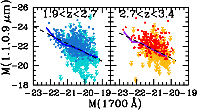
Figure 14.— Rest-frame $1.1$ and $0.9$ $\mu$m absolute magnitudes (from IRAC channel 1 data) vs. UV absolute magnitude for 630 spectroscopically confirmed galaxies at redshifts $1.4\leq z<2.7$ (left) and 344 spectroscopically confirmed galaxies at redshifts $2.7\leq z<3.7$ (right). Points and downward-pointing arrows denote galaxies detected and undetected (to $3\sigma$), respectively, at $3.6$ $\mu$m, and the solid lines denote the stacked magnitudes as a function of UV luminosity (Table 8). The dashed lines show the best-fit linear relations obtained from the Buckley-James estimator, taking into account both IRAC detections and nondetections.

As discussed in Appendix C, the conversion between near-IR magnitude and stellar mass depends on UV luminosity, simply because current star formation can contribute to the near-IR magnitude. To properly account for this effect, we converted the near-IR magnitude found for each bin of UV luminosity to a stellar mass using the relation between near-IR magnitude and stellar mass appropriate for that bin of UV luminosity (see Appendix C, Figure 28, and Table 7). In this way, we are able to account for the star formation history of the average galaxy at a given UV luminosity in estimating its stellar mass.

Figure 16 shows the resulting median stellar masses of galaxies in different UV magnitude bins. For comparison, the dashed lines show the results at $z\sim 2.30$ and $z\sim 3.05$ if we assume a single best-fit linear relation between $M_{\ast}$ and $M_{1.1,0.9}$ for all galaxies (irrespective of UV luminosity). Interestingly, it is primarily for galaxies brighter than $L^{\ast}_{\rm UV}$ that the SFR is significant enough to bias the $M_{\ast}$ versus near-IR relation towards higher masses. Below $L^{\ast}$, the discrepancy in stellar masses derived using relation for all galaxies versus that derived using the relation only for UV faint galaxies, is small. This can be attributed to the fact that the former relation is dominated by UV faint galaxies at fainter near-IR magnitudes (Appendix C and Figure 27). The relationship between UV luminosity and mass is similar to that derived in Sawicki (2011) for a sample of BX selected galaxies in the Hubble Deep Field (HDF) North, once we have taken into account differences in SED fitting by remodeling our galaxies using the same templates (Bruzual & Charlot, 2003) used in that study.

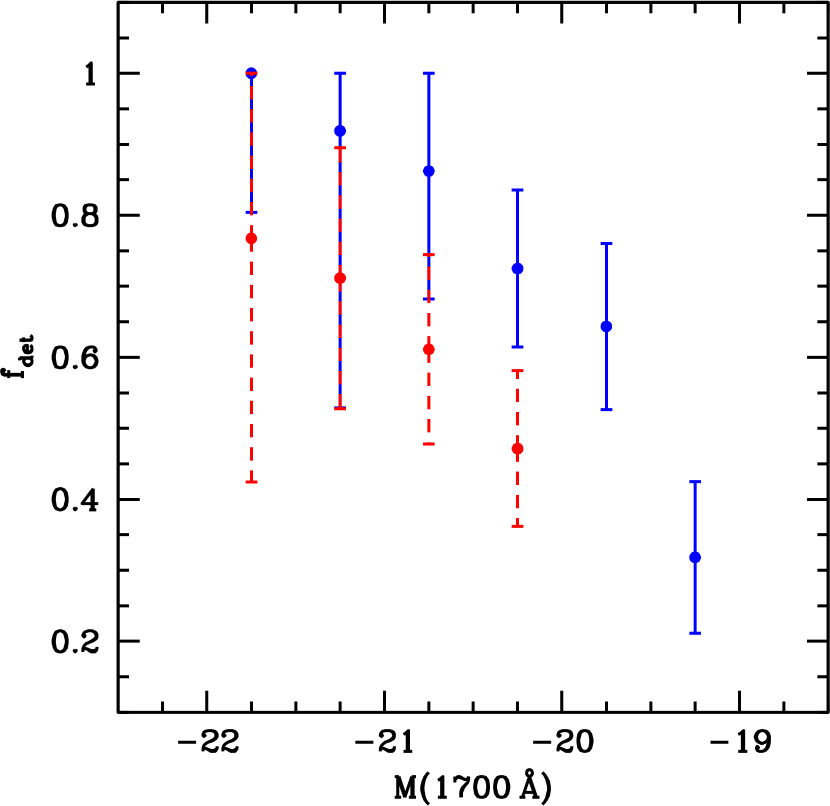
Figure 15.— Fraction of galaxies detected in IRAC channel 1 ($3.6$ $\mu$m) as a function of absolute magnitude at $1700$ Å, at redshifts $1.4\leq z<2.7$ (blue) and $2.7\leq z<3.7$ (red). Errorbars reflect Poisson statistics.

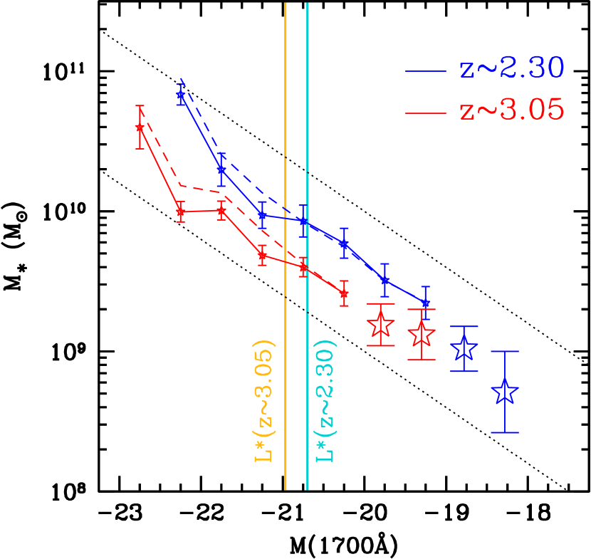
Figure 16.— Median stellar mass, inferred from stacking the IRAC data, in bins of UV absolute magnitude (points and solid lines). The stacked IRAC magnitudes were converted to stellar mass assuming the best-fit linear relations between these two quantities in bins of UV magnitude (Appendix C, Figure 28, Table 7). Results are also shown (dashed lines) where we have assumed a single best-fit linear relation for all galaxies in our sample. The vertical lines denote the values of $L^{\ast}$ of the UV luminosity functions at $z\sim 2.30$ and $z\sim 3.05$ (Reddy & Steidel, 2009). The open stars denote the median stellar mass in the bins of UV faint photometrically selected galaxies. The conversion between near-IR magnitude and stellar mass for these faint bins is discussed in Appendix C. The dotted black lines indicate lines of constant $M/L$ ratio.

Table 5Stacked IRAC Magnitudes for UV faint Sample

Redshift Interval	M(1700Å) Range	$3.6$ $\mu$m	$4.5$ $\mu$m
$1.4\leq z<2.7$	-19.03     -18.53	$-19.97\pm 0.10$ (393)	$-20.09\pm 0.09$ (260)
	-18.53     -18.03	$-19.28\pm 0.26$ (170)	$-19.24\pm 0.34$ (112)
$2.7\leq z<3.7$	-20.05     -19.55	$-20.54\pm 0.08$ (386)	$-20.64\pm 0.06$ (251)
	-19.55     -19.05	$-20.29\pm 0.13$ (230)	$-20.08\pm 0.32$ (132)

The results summarized in Figures 14 and 16 imply that even within the limited dynamic range of UV luminosity probed with the spectroscopic sample, there is a steep trend of mean stellar mass with UV luminosity. The UV faintest galaxies in our spectroscopic sample (around $0.16L^{\ast}$) have mean stellar masses that are at least a factor of $\approx 40$ smaller than those measured for UV-bright galaxies with $M_{\rm 1700}\simeq-22.5$. This steep trend is only evident once galaxies undetected in the near-IR are included (Figure 14); the trend is much shallower or non-existent when examining only those galaxies detected in $K_{\rm s}$-band or with IRAC (Shapley et al., 2001, 2005). Similar trends between UV luminosity and stellar mass have been found for dropout selected galaxies at higher redshifts (Stark et al., 2009; Lee et al., 2011a), and could be inferred from the fact that the SFR correlates with both UV luminosity (Appendix B) and stellar mass (Figure 12).

7.2.2 Stellar Masses of Photometrically Selected UV Faint Galaxies

To extend these spectroscopic results to fainter UV luminosities, we have stacked the IRAC data for photometrically selected BXs and LBGs with ${\cal R}>25.5$, specifically in two bins with $25.5<{\cal R}<26.5$ and $26.5\leq{\cal R}<27.0$, using the same stacking method discussed in Appendix D. These photometrically selected faint galaxies are likely to lie at the redshifts of interest, given the strong correlation between contamination fraction and UV magnitude (Reddy et al., 2008; Reddy & Steidel, 2009). Table 5 lists the stacked $3.6$ and $4.5$ $\mu$m fluxes for these faint bins, along with the number of objects contributing to the stacks. The relatively faint stacked IRAC magnitudes obtained for these galaxies suggests that low redshift contaminants, if they exist, do not dominate the signal; otherwise, we would have expected the stacked IRAC flux to be brighter than the observed value. The near-IR magnitudes are converted to stellar masses as described in Appendix C. These faint stacks imply that the trend between stellar mass and UV luminosity derived from the spectroscopic sample extends to fainter UV magnitudes and lower masses (Figure 16).

Having computed their mean stellar masses, we examine the UV faint galaxies in the context of the SFR-$M_{\ast}$ relation. The unattenuated SFRs implied by the mean UV luminosities of the two bins of photometrically selected faint galaxies at $z\sim 2.3$ are $\approx 2$ and $1$ M_⊙ yr^-1. The average UV slopes for these two bins, based on the relationship between $\beta$ and $M_{\rm UV}$ at $z\sim 2.5$ (Bouwens et al., 2011a), are $\langle\beta\rangle\approx-1.8$ and $-1.9$. Converting these $\beta$ to dust obscurations with the Meurer et al. (1999) relation and applying them to the unobscured (UV) SFRs then implies bolometric SFRs of $\approx 5$ and $3$ M_⊙ yr^-1. The dispersion in $\beta$ for a given $M_{\rm UV}$ results in a factor of $\approx 2$ uncertainty in these SFRs. Adding the intrinsic scatter in the Meurer et al. (1999) relation increases the SFR uncertainties to a factor of $\approx 2.3$. Figure 12 includes the values of inferred bolometric SFR for the faint samples analyzed here.

Given the biases discussed in Sections 6.4, 7, and Appendices B and C, it is prudent to determine whether the location of the UV faint galaxies on the SFR-$M_{\ast}$ plane may be biased with respect to all galaxies that lie within the same bins of stellar mass. We investigate such biases using simulations that are presented in Appendix E. The first main result of our simulations is that Malmquist bias can result in overestimated mean SFRs in bins of stellar mass. One may circumvent this bias by stacking in bins of SFR (or UV luminosity), at the expense of probing the intrinsic SFR-$M_{\ast}$ relation over a narrower range of $M_{\ast}$ where the flux-limited sample is complete. The critical point is that the median stellar mass in bins of SFR may not directly translate to the median SFR in that same bin of stellar mass. Secondly, in an ideal situation, it is desirable to perform full SED fitting for all galaxies in a sample, in order to better constrain stellar masses that take into account the star formation history and current SFR. In our case, a substantial fraction of galaxies in our sample are faint (and low mass) and are undetected longward of the Balmer and $4000$ Å  breaks. One can estimate stellar masses for such objects by assuming some $M/L$ ratio. However, as we have shown, a proper treatment must take into account the UV luminosity dependence of the near-IR $M/L$ ratio when estimating stellar masses for undetected objects (or objects detected in stack). Having accounted for these biases, we find that, within the uncertainties of the faint stacks, the SFR-$M_{\ast}$ relation exhibits a close to unity slope to stellar masses as low as $M_{\ast}\simeq 5\times 10^{8}$ M_⊙. Progress in quantifying any possible evolution of the SFR-$M_{\ast}$ relation at low masses should be made with future spectroscopic observations of larger samples of UV faint galaxies, combined with information from deep near-IR selected samples.

8. DISCUSSION

A principal aspect of our analysis is the comparison of SED-inferred SFRs to those determined from direct measurements of dusty star formation at $z\sim 2$. An important conclusion of our analysis is that exponentially declining star formation histories yield SFRs that are inconsistent with those obtained by combining mid-IR and UV data. While both the constant and rising star formation histories yield SFRs that consistent with the independent measurements, as we discuss below, there is additional evidence that suggests that on average galaxies at $z\gtrsim 2$ have SFRs that may be increasing with time.

8.1. The Typical Star Formation History of High-redshift Galaxies

The SED determined SFRs, and those computed from combining mid-IR and UV data, vary roughly linearly with stellar mass (Figure 12). Hence, as shown in Figure 17, the specific star formation $\phi\equiv{\rm SFR}/M_{\ast}$ of galaxies with $1.5\leq z_{\rm spec}\leq 2.6$ is roughly constant over $\approx 2.4$ orders of magnitude in stellar mass up to $\log[M_{\ast}/{\rm M}_{\odot}]=11.0$, with a weighted mean of $\phi(z\sim 2)=2.4\pm 0.1$ Gyr^-1, as measured from SFRs[IR+UV]. SFRs[SED] for galaxies with $2.7\leq z\leq 3.7$ imply $\phi(z\sim 3)=2.3\pm 0.1$ Gyr^-1. Similar values of $\phi$ are obtained if we assume a CSF model for deriving the SFRs[SED] and/or stellar masses.

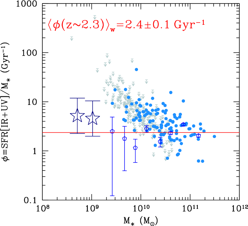
Figure 17.— Specific SFR, $\phi\equiv{\rm SFR}/M_{\ast}$, as a function of stellar mass for the MIPS sample of galaxies with redshifts $1.5\leq z\leq 2.6$. Detections and non-detections are indicated by the filled symbols and downward arrows, respectively. The mean specific SFR in bins of stellar mass for the spectroscopic sample and photometrically selected UV faint sample are indicated by the small open pentagons and large open stars, respectively. The weighted mean specific SFR over all stellar masses is $\langle\phi\rangle=2.4\pm 0.1$ Gyr^-1, denoted by the solid line.

Several determinations of the specific SFR at low and high redshift, nominally derived at a fixed stellar mass of $5\times 10^{9}$ M_⊙, are compiled in Figure 18. The average specific SFRs derived at $z\sim 2$ and $z\sim 3$ are similar to those measured at redshifts $z>3$ (e.g., Daddi et al. 2007; Stark et al. 2009; González et al. 2010); including dust corrections to these higher redshift points results in a roughly constant specific SFR at $z\gtrsim 4$ (Bouwens et al., 2011a), and one which is about a factor of $2-3$ larger than the values we find at $z\sim 2-3$. A note of caution regarding these higher redshift ($z\gtrsim 3$) results is that the relatively young age of the universe implies a limited dynamic range in $M/L$ ratio, translating to a limited range in the possible simple star formation histories. As such, it is perhaps not at all surprising to find SFR $\propto M_{\ast}$, given that the young stars that dominate the UV continuum also contribute significantly to the rest-optical flux, the latter of which is used to constrain the stellar mass (i.e., the “outshining” problem as discussed earlier). This degeneracy may also lead to an artificial tightening of the scatter in the SFR-$M_{\ast}$ relation at high redshift. The advantage of the method employed here, for $z\sim 2$ galaxies, is that we have (a) determined SFRs largely independent of the SED modeling (and hence $M_{\ast}$) by incorporating the MIPS $24$ $\mu$m data, and (b) the stellar masses are constrained with IRAC data that probe the peak of the stellar emission at $1.6$ $\mu$m.

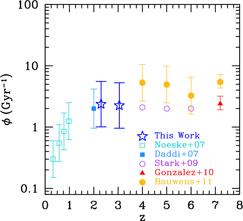
Figure 18.— Evolution of specific SFR $\phi$ as function of redshift for galaxies of a stellar mass $M_{\ast}\simeq 5\times 10^{9}$ M_⊙. Data are taken from the compilation of González et al. (2010), which includes values from Noeske et al. (2007), Daddi et al. (2007), Stark et al. (2009), and González et al. (2010). We also show the dust corrected values from Bouwens et al. (2011a). The rms scatter in the specific SFR at a given mass is taken to be $0.3$ dex for the Noeske et al. (2007) points, $0.32$ dex for the Daddi et al. (2007) point, $\approx 0.3$ dex for the dust-corrected values at $4.0\lesssim z\lesssim 6$ from Bouwens et al. (2011a), and $\approx 0.10$ dex for the González et al. (2010) point at $z\sim 7$. For our determination at $z\sim 2.3$, we compute a scatter of $\approx 0.37$ dex from a survival analysis that includes MIPS $24$ $\mu$m non-detections (see text; note that this is the scatter of individual galaxies about the mean specific SFR, not the error in the mean specific SFR). A similar value of the scatter is adopted for the $z\sim 3$ determination.

While independent estimates of SFRs are not practical at $z\gtrsim 3$ given the general faintness of galaxies and their expectation of having lower dust content, we note that: (a) the mean specific SFR at $z\sim 2$ is similar to that derived at higher redshift, despite the different methods used to measure SFRs at $z\sim 2$ versus $z\gtrsim 3$ and (b) there is well-defined correlation between SFR and $M_{\ast}$ as $z\lesssim 2$ (Noeske et al., 2007), where SED modeling independent measurements of SFRs can be obtained and where rest-frame near-IR constraints on stellar mass are accessible. By extension, these lower redshift results hint that there may indeed be an intrinsic correlation between SFR and $M^{\ast}$ at the highest redshifts. Regardless, we note that if the stellar masses are severely biased for large numbers of galaxies at $z\gtrsim 3$ (due to “contamination” of the rest-optical light from the most massive stars), then correcting for this effect result in stellar mass densities at $z\gtrsim 4$ that would be inconsistent with the integrated star formation history inferred at these early cosmic times (e.g., Reddy & Steidel 2009; Bouwens et al. 2011a). Such an inconsistency would be made even worse if we then also corrected the stellar mass determinations at $z\gtrsim 4$ for the effect of strong emission line contribution to the broadband optical fluxes (Schaerer & de Barros, 2009, 2010). With this in mind, we find that even with the Bouwens et al. (2011a) dust corrections, the overall picture does not change significantly and the specific star formation rates appear to have remained approximately constant, within a factor of a few, over the $2.5$ Gyr interval from $z=7$ to 2. As such, the average SFRs would be roughly proportional to stellar mass, implying that both increase exponentially with time.

8.1.1 Expectations from a Constant Star Formation History

Given this suggestion, it is useful to place the $z\sim 2-3$ galaxies in the context of higher redshift samples by evolving their SFRs backward in time. For a CSF history, the specific SFR will be larger at earlier times. For example, a typical galaxy at redshift $z=2.3$ with $\phi\approx 2.4$ Gyr^-1 would have had $\phi\gtrsim 30$ Gyr^-1 at $z\gtrsim 2.65$, $\approx 390$ Myr earlier. The upper redshift $z=2.65$ is close the upper boundary where the $24$ $\mu$m data are still sensitive to the rest-frame $8$ $\mu$m emission, and the difference in time between $z=2.3$ and $z=2.65$ of $\approx 390$ Myr is similar to the mean “age” determined for our spectroscopic sample of $z\sim 2$ galaxies (Figure 9). Extending to higher redshift, the specific star formation would increase by more than an order of magnitude in the $\approx 80$ Myr between $z=2.60$ and $z=2.68$, reaching a value of $\phi\approx 180$ Gyr^-1 at this latter redshift (Figure 19). Our sample, which encompasses this higher redshift ($z=2.68$), includes very few galaxies with $\phi$ as large as the one predicted with a CSF history. The lack of galaxies with such high specific SFRs is unlikely to be a selection effect because the SFR would remain unchanged and such galaxies should still be selectable via their UV emission. If anything, the higher redshift progenitors of galaxies at $z\sim 2$ would be more easily detectable via their UV emission at the same SFR given that the extinction per unit bolometric SFR decreases with increasing redshift (Reddy et al., 2010). Hence, there appears to be a true paucity of galaxies with specific SFRs $\phi\gtrsim 100$ Gyr^-1 relative to what we would have predicted if the majority of galaxies at $z=2.3$ had CSF (or declining) histories. Stated another way, the relatively small scatter in the SFR at a given stellar mass over the entire redshift range $1.5\lesssim z\lesssim 2.6$ precludes the possibility that there exists a large population of galaxies with specific SFRs that are substantially larger than the mean values observed at these epochs. These mean values of $\phi$ are roughly independent of stellar mass with $\langle\phi\rangle\approx 2.4$ Gyr^-1 (i.e., the lower mass progenitors of $z=2.3$ galaxies retain roughly the same specific SFR, contrary to our expectation if galaxies were evolving with a constant SFR).

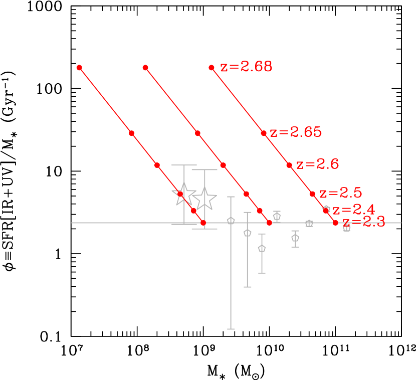
Figure 19.— Same as Figure 17, where median stacks of the specific SFR are shown by the grey points (individual points have been suppressed for clarity). The connected red points show the evolution in $\phi$ and $M_{\ast}$ of a galaxy with $M_{\ast}=10^{9}$, $10^{10}$, and $10^{11}$ M_⊙ and $\phi=2.4$ Gyr^-1 at $z=2.3$, assuming a CSF history.

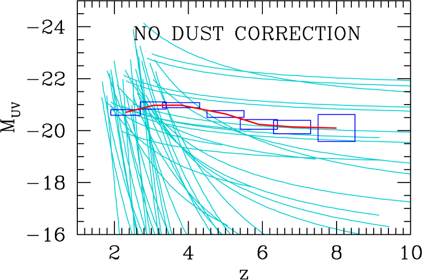
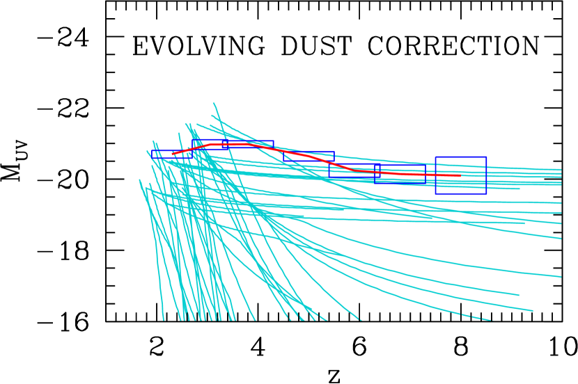
Figure 20.— Intrinsic (left) and observed (right) absolute UV magnitude as a function of redshift for 45 galaxies chosen randomly from our SED sample. The curves assume a star formation history where the specific SFR $\phi$ is constant. The intrinsic UV magnitude is derived directly from the bolometric SFR without any correction for dust. The observed UV magnitude is computed under the assumption that the dust correction depends on the observed UV magnitude (Reddy & Steidel, 2009; Bouwens et al., 2011a). The rectangles and red line indicate the values and uncertainties in the characteristic absolute magnitude $M_{\rm UV}^{\ast}$ derived from the $z\sim 3.8-8.0$ luminosity functions of Bouwens et al. (2011b) assuming $\delta z\approx 1$; and the $z\sim 2-3$ luminosity functions of Reddy & Steidel (2009) assuming $\delta z=0.8$ and $0.7$ at $z\sim 2.30$ and $z\sim 3.05$, respectively.

8.1.2 Expectations from a Rising Star Formation History and Implications for the Evolution of $M_{\rm UV}$ with Redshift

As discussed in Section 6.2, a rising star formation history where the specific SFR $\phi$ is roughly constant implies “ages” that can be arbitrarily old if we vary the normalization of the star formation history. Given such a star formation history, we can estimate the redshift evolution in UV luminosity for each of the galaxies in our sample. For clarity, we show this evolution for a subset of 45 galaxies drawn randomly from our SED sample of 1959 galaxies, assuming ages that are either $2$ Gyr or $2.5$ Gyr, depending on the redshift of the galaxy (so as not to violate the age of the universe at each redshift), in Figure 20. The observed UV magnitudes are calculated assuming that the dust extinction varies with total SFR (or intrinsic UV luminosity; e.g. Reddy et al. 2008; Bouwens et al. 2009; Reddy et al. 2010). We adopted the relation between UV luminosity and bolometric luminosity in order to apply this correction (see Appendix B; adopting the Bouwens et al. 2009 or Bouwens et al. 2011a relations between UV slope, $\beta$, and $M_{\rm UV}$ at $z\sim 2.5$ yields similar results). The correction is renormalized to yield the same dust reddening as indicated by the best-fit value of $E(B-V)$ from the SED fitting. For comparison, we also show the maximum possible UV luminosity (i.e., assuming no dust reddening) as a function of redshift in the left panel of Figure 20. Hence, the curves shown in the left and right panels of Figure 20 should encompass the full range of possible $M_{\rm UV}$ versus redshift tracks for each object. Also shown are the characteristic magnitudes $M_{\rm UV}^{\ast}$ of the UV luminosity functions at $z\sim 2-3$ from Reddy & Steidel (2009) and $z\sim 4-8$ from Bouwens et al. (2011b).

In the case of rising SFRs, the redshift evolution in $M_{\rm UV}$ for $z\sim 2-3$ galaxies with ${\cal R}<25.5$ implies that a substantial fraction of them would have been fainter than $L^{\ast}$ (i.e., having sub-$L^{\ast}$ luminosities) at $z\gtrsim 4$. Hence, the progenitors of $z\sim 2-3$ galaxies are likely to have appeared as sub-$L^{\ast}$ galaxies in dropout samples at $z\gtrsim 4$. Further, the mean specific SFR of $\langle\phi\rangle\simeq 2.4$ Gyr^-1 at $z\sim 2$ implies a mass doubling time of $\approx 300$ Myr (Equation 4). Hence, a typical star-forming galaxy at $z=2.3$ has doubled its stellar mass since $z=2.8$. Similarly, a $z=2.3$ galaxy would have had a fifth of its current stellar mass (and an intrinsic UV luminosity that is $\approx 1.25$ mag fainter) at $z=3.0$ (e.g., Figures 16 and 20).

At face value, the average rising star formation history characteristic of typical star-forming galaxies at $z\sim 2$ would imply a significant evolution in $L^{\ast}$ of the UV luminosity function at higher redshifts. While this is true above $z\sim 4$, in the sense that $L^{\ast}$ becomes progressively brighter with decreasing redshift from $z\sim 7$ to $z\sim 4$ (e.g., Bouwens et al. 2011b), recent studies suggest little evolution in $L^{\ast}$ over the redshift range $z\sim 2-4$ (Reddy & Steidel, 2009). How can we reconcile the rising star formation histories of $z\sim 2$ galaxies with the fact that $L^{\ast}$ does not evolve significantly between $z\sim 2-4$? There are two possible explanations. First, observations indicate the emergence of a population of massive and passively evolving galaxies over these redshifts (van Dokkum et al., 2006), implying that some fraction of UV-bright galaxies eventually “turn off” by $z\sim 2$ (Stark et al., 2009).

Second, there is a non-monotonic relationship between bolometric and UV luminosity for $z\sim 2$ galaxies, in the sense that as the bolometric SFR of galaxy increases, dust attenuation will also increase, and eventually there is a point at which the observed UV luminosity saturates Reddy et al. (2010). In effect, dust obscuration limits the maximum observable UV luminosity of galaxy which, for $z\sim 2$ galaxies, occurs around the value of $L^{\ast}$. Therefore, as a galaxy’s SFR increases with time, there comes a point at which dust attenuation becomes large enough that its observed UV luminosity no longer increases with increasing SFR. It is likely that some combination of aforementioned effects (i.e., the fading of some fraction of UV-bright galaxies between $z\sim 4$ and $z\sim 2$, and the limit to the observed UV luminosity due to dust attenuation; e.g. see also Bouwens et al. 2009) conspire to produce a relatively constant value of $L^{\ast}$ between $z\sim 2-4$, even though the average star formation history may be rising during these epochs.

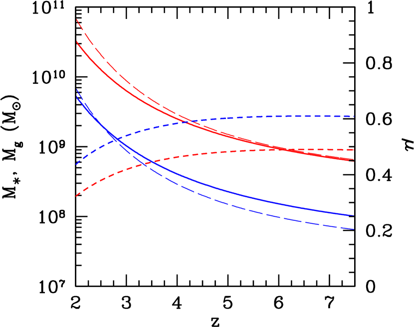
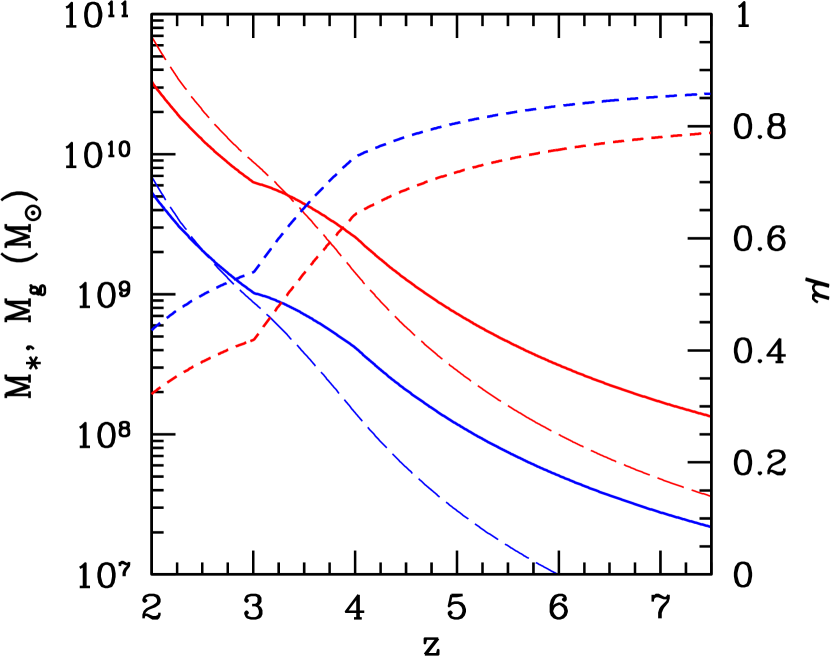
Figure 21.— Left: Redshift evolution in gas (solid lines) and stellar (long dashed lines) masses for galaxies with a final stellar mass of $\log M_{\ast}=9.5$ and 10.5 at $z\sim 2.3$, assuming a constant specific SFR of $\phi=2.4$ Gyr^-1. Also indicated (short dashed lines) is the evolution in gas mass fraction for these two examples. Right: Same as left panel where we have assumed $\phi\simeq 2.4$ Gyr^-1 at $z\lesssim 3.0$ based on our sample, and $\phi\simeq 5.0$ Gyr^-1 at $z\gtrsim 4$ based on the dust-corrected specific SFRs presented by Bouwens et al. (2011a). We have used a spline fit to interpolate the specific SFRs over the redshift range $3.0\lesssim z\lesssim 4.0$.

8.2. Implications for Cold Gas Accretion at High Redshift

In Reddy et al. (2006b), we examined the relationship between specific SFR, $\phi$, and cold gas mass fraction, $\mu$:

$$\phi=C\frac{\mu^{1.4}}{1-\mu},$$ (7)

where we assumed the Kennicutt-Schmidt relation (Kennicutt, 1998) between SFR surface density and cold gas mass surface density. The multiplicative factor $C$ in the equation above depends on the constant of proportionality between SFR and cold gas mass surface density and the size of the star-forming region. We have defined the cold gas mass fraction $\mu$ as

$$\mu\equiv\frac{M_{\rm g}}{M_{\rm g}+M_{\ast}}.$$ (8)

We revisit this relationship in light of our new determinations of the specific SFRs of $z\sim 2-3$ galaxies. The Kennicutt (1998) relation between SFR and cold gas mass surface density reduces to

$$M_{\rm g}\simeq 5.2\times 10^{8}\left[\frac{\Psi}{\rm M_{\odot}\,yr^{-1}}\right]^{\frac{1}{N}}\left[\frac{r_{\rm 1/2}}{\rm kpc}\right]^{2-\frac{2}{N}}\,{\rm M_{\odot}},$$ (9)

where $M_{\rm g}$ is the cold gas mass is solar masses, $\Psi$ is the SFR, $r_{\rm 1/2}$ is the half-light radius characterizing the size of the star-forming region, and the power law index of the Kennicutt-Schmidt relation is $N=1.4$ (below, we explore how changing the value of $N$ affects our results). Law et al. (2012) have quantified the sizes and their redshift evolution of a subset of the UV selected galaxies in the SED sample that have HST/WFC3 IR imaging. These authors find characteristic half-light radii of $r_{\rm 1/2}\approx 1.3$ and $1.8$ kpc for $z\sim 2$ galaxies in stellar mass bins centered at $\log(M_{\ast}/M_{\odot})=9.5$ and $10.5$, respectively. These sizes are measured in the rest-frame optical and are roughly $20\%$ smaller than those measured in the rest-UV, where the latter may be more appropriate for the size of the star-forming regions. Law et al. (2012) also find $r_{\rm 1/2}\propto(1+z)^{\gamma}$ where $\gamma\approx-1.07$, measured from $z=3.6$ to $z=1.5$. This size scaling with a power law close to unity is similar to that inferred from higher redshift ($z\gtrsim 4$) dropout samples (Oesch et al., 2010), and is indistinguishable within the errors from the $r_{\rm 1/2}\propto H(z)^{-1}$ scaling proposed by Ferguson et al. (2004). In the subsequent discussion, we assume the results of Law et al. (2012) for the redshift evolution in the characteristic half-light radii measured in the rest-frame UV.

Adopting Equation 9, we show in Figure 21 the evolution of the cold gas masses for a typical star-forming galaxy with a constant specific SFR of $\phi=2.4$ Gyr^-1 (and, hence, an exponentially rising star formation history with $\tau_{\rm r}=\phi^{-1}\simeq 400$ Myr) and (final) stellar mass at $z\sim 2.3$ of $\log(M_{\ast}^{z=2.3}/M_{\odot})=9.5$ and $10.5$ (denoted by the solid lines in the left panel of Figure 21). Also shown (in the right panel of Figure 21) is the inferred evolution assuming a median specific SFR that evolves with redshift: at $z\sim 2-3$ we assume $\phi\simeq 2.4$ Gyr^-1, based on our sample; at $z\gtrsim 4$ we assume $\phi\simeq 5.0$ Gyr^-1, based on the dust-corrected specific SFRs found by Bouwens et al. (2011a). We have adopted a spline fit to these values in order to infer the specific SFR over the range $3.0\lesssim z\lesssim 4.0$. In addition, the stellar masses are evolved backwards in time assuming a gas recycling rate from stellar remnants as computed from the CB11 stellar population synthesis models for an exponentially rising star formation history with $\tau_{\rm r}\simeq 400$ Myr.

There are several important implications of these results. Qualitatively, the inferred evolution assuming a constant and evolving median specific SFR (left and right panels, respectively, of Figure 21) are similar. If we assume that the Kennicutt-Schmidt relation applies at high redshift, then a rising SFR must be accompanied by an increase in cold gas surface density. Hence, the cold gas mass should increase as $\approx M_{\ast}^{5/7}$, assuming a Schmidt law index of $N=1.4$. The cold gas mass fraction, $\mu$, will therefore evolve with time more slowly than if the SFR is constant or declining exponentially. The results of Figure 21 indicate that the characteristic cold gas mass fraction (assuming $\phi=2.4$ Gyr^-1) is relatively constant above $z\sim 4$, and declines more rapidly at lower redshift. The average stellar mass of galaxies in our spectroscopically confirmed sample at $1.4\leq z\leq 2.7$ is $\langle M_{\ast}\rangle=1.6\times 10^{10}$ M_⊙ (see Section 6.1). For this stellar mass, the cold gas fraction is inferred to be between $50\%-60\%$ at $z\gtrsim 4$ assuming $\phi=2.4$ Gyr^-1 (or $\gtrsim 60\%$ at $z\gtrsim 4$ assuming the dust corrected $\phi$ of Bouwens et al. 2011a), and decline to $\approx 40\%-50\%$ at $z\approx 2.8$. More generally, on an object by object basis, we find a large range in cold gas fraction at $z\sim 2$, with typical values of $\mu\simeq 0.4-0.6$. This is quite similar to the average cold gas fractions of $\mu\simeq 0.3-0.6$ inferred for star-forming galaxies with similar stellar masses as represented in our spectroscopic sample (Figure 9) at $z\sim 2$ based either on dust-corrected H$\alpha$ (via the Kennicutt-Schmidt relation; Erb et al. 2006b) or CO measurements (e.g., Daddi et al. 2010; Tacconi et al. 2010; Riechers et al. 2010; see also Papovich et al. 2011).

As we have just discussed, the mean cold gas fraction is likely higher at $z\sim 4$ than at $z\sim 2$, and the mean fraction may not evolve strongly above $z\sim 4$ for typical star-forming galaxies at these higher redshifts (e.g., stronger evolution may be expected for galaxies with larger stellar masses). To illustrate these issues further, we show in Figure 22 the net cold gas accretion rates (as inferred from the specific SFRs) and SFRs for galaxies that have $M_{\ast}^{z=2.3}=10^{8}$, $10^{9}$, $10^{10}$, and $10^{11}$ M_⊙ by $z\sim 2.3$, adopting the evolution in $\phi$ that was assumed in the left panel of Figure 21. We computed the net cold gas accretion rate as $\dot{M}^{\rm cold}_{\rm acc}$, which is related simply to: (a) the amount of cold gas consumed to form stars in a time $\delta t$ (i.e., the SFR); (b) the time derivative of the cold gas mass (computed from Equation 9); and (c) the rate at which the mass formed in stars is released back into the ISM as computed from the CB11 stellar population synthesis models ($\dot{R}$). For a Salpeter IMF, the CB11 models indicate that the fraction of gas returned to the ISM to the stellar mass reaches a value of $\approx 30\%$ at 2 Gyr, assuming an exponentially rising star formation history with $\tau_{\rm r}\simeq 400$ Myr. Hence, we can write the net cold gas accretion rate as

$$\dot{M}^{\rm cold}_{\rm acc}=\dot{M}_{\rm g}+\Psi-\dot{R}$$ (10)

(see also Equation 8 of Papovich et al. 2011).

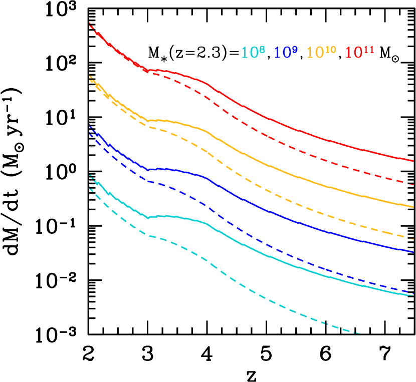
Figure 22.— Redshift evolution in the SFR (dashed lines) and net cold gas accretion rate (solid lines) for galaxies with final stellar masses at $z\sim 2.3$ $M_{\ast}^{z=2.3}=10^{8}$, $10^{9}$, $10^{10}$, and $10^{11}$ M_⊙. The curves assume a specific SFR that evolves from $\phi\simeq 2.4$ Gyr^-1 at $z\sim 2-3$ to $\phi\simeq 5.0$ Gyr^-1 at $z\gtrsim 4$ and a gas recycling rate from stellar remnants computed from the CB11 stellar population synthesis models for a exponentially rising star formation history with $\tau_{\rm r}\simeq 400$ Myr.

Above $z\sim 4$, the net cold gas accretion rate outpaces the SFR by at least a factor of two, with the difference between cold gas accretion rate and SFR being largest for lower mass galaxies at any given redshift above $z\sim 3-4$. It is evident that the SFR becomes comparable to the net cold gas accretion rate at a redshift which is dependent upon stellar mass (i.e., the redshift where the dashed and solid lines come together in Figure 22). In particular, $\Psi\approx\dot{M}^{\rm cold}_{\rm acc}$ at higher redshifts for galaxies with larger stellar masses.

Above $z\sim 2-3$, the accretion rate outpaces the SFR and the average cold gas fraction remains consistently high (e.g., right panel of Figure 21; Bouché et al. 2010; see also Figure 4 of Papovich et al. 2011). Of course, the actual dispersion in $\mu$ at a given redshift (even above $z\sim 4$) may still be quite large. Nonetheless, the steep UV luminosity function at $z\gtrsim 4$ (e.g., Bouwens et al. 2009) implies that less UV luminous and hence lower stellar mass galaxies (e.g., Stark et al. 2009; Lee et al. 2011a, b; see also Figure 14) should dominate, and hence the number-weighted mean cold gas fraction at these redshifts should be quite high with $\mu\gtrsim 60\%$ (Figure 21). Finally, we note that the difference in $\dot{M}^{\rm cold}_{\rm acc}$ and SFR will be slightly larger at $z\gtrsim 4$ had we assumed a shallower slope of the Schmidt (1959) relation of $N\simeq 1.1-1.2$ (e.g., as suggested by Genzel et al. 2010), with a further result being that the point at which $\Psi\approx\dot{M}^{\rm cold}_{\rm acc}$ shifts to lower redshifts for galaxies of a given stellar mass.

The physical picture implied by the redshift evolution in cold gas accretion is that on average galaxies must be continually accreting gas to support their increasing SFRs. Indeed, the gas consumption timescales assuming a CSF history for $z\sim 2$ UV selected galaxies are on average a factor of two lower than median stellar ages, implying that significant gas accretion must be occurring at $z\sim 2$ (Erb, 2008), while at the same time, such galaxies are inferred from clustering measurements to have long duty cycles (e.g., Conroy et al. 2008). A high rate of gas accretion is also required to explain the increasing SFRs (and SFR density) contributed by galaxies of a fixed number density at $z\gtrsim 4$ (Papovich et al., 2011).

We conclude with a caution against over-interpreting the physical implications of the redshift at which $\Psi\approx\dot{M}^{\rm cold}_{\rm acc}$. One might speculate that below this redshift–which for typical galaxies with $M_{\ast}\gtrsim 10^{9}$ M_⊙ occurs around $z\sim 2$ (Figure 22)—the SFR declines primarily in response to a lower cold gas accretion rate. While this may be the case—and would explain naturally the overall decline in the cosmic SFR density at the same redshifts ($z\sim 2$)—as we discuss in the next section, the cold gas accretion computed above evidently constitutes only a small fraction of the total baryons accreted onto halos. Therefore, some other mechanism(s) must be responsible for regulating the large number of baryons that never end up in stars at high redshift. We discuss this further in Section 8.3.

8.3. A Consideration of Gas Inflows, Outflows, and the Expectations from Simulations

So far, we have not distinguished between gas inflows and outflows, and have only referred to the net cold gas accretion rate as inferred from the specific SFRs of $z\gtrsim 2$ galaxies. We can estimate the cold gas inflow rate by making some assumptions of the gas outflow rate. Taking the net cold gas accretion rate as the difference between inflow ($\dot{M}_{\rm in}$) and outflow rates ($\dot{M}_{\rm out}$), and assuming that $\dot{M}_{\rm out}=\eta_{\rm out}\Psi$, where $\eta_{\rm out}$ is commonly referred to as the “mass-loading factor,”  we can rewrite Equation 10:

$$\dot{M}_{\rm in}=\dot{M}_{\rm g}+(1+\eta_{\rm out})\Psi-\dot{R}.$$ (11)

Direct measurements of $\eta_{\rm out}$ in high-redshift galaxies are sparse, given the difficulty of measuring the covering fraction and terminal velocity of the gas and its radial extent, as well as the HI column density (due to saturation of the typical absorption lines used to make such measurements). Pettini et al. (2002) estimated the mass outflow rate of the low-ionization and HI gas of the lensed Lyman Break galaxy cB58, finding $\eta_{\rm out}\simeq 1.75$. This is likely a lower limit because a significant fraction of the outflowing gas may be at higher velocity and/or in a more highly ionized state. Alternatively, Erb (2008) finds that $\eta_{\rm out}\simeq 1$ is required to reproduce the mass-metallicity relation at $z\sim 2$. From the theoretical standpoint, hydrodynamical simulations find mean mass-loading factors of at least a factor of a few for galaxies with stellar masses at the low end of those found in our sample ($M_{\ast}\sim 10^{9}$ M_⊙), and being less than unity for the most massive galaxies (Oppenheimer & Davé, 2006, 2008; Finlator & Davé, 2008; Oppenheimer et al., 2011; Davé et al., 2011). To encompass the range of observed and expected mass outflow rates, we consider the effect of changing $\eta_{\rm out}$ on the cold gas inflow rate inferred for a typical galaxy in our sample with $M^{z=2.3}_{\ast}\simeq 1.6\times 10^{10}$ M_⊙ , as shown in Figure 23.

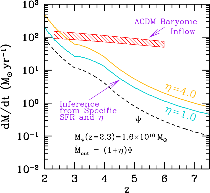
Figure 23.— SFR (dashed line) and inferred cold gas inflow rates (solid lines) for different values of the mass-loading factor $\eta$, for a galaxy with a final stellar mass of $M_{\ast}=1.6\times 10^{10}$ M_⊙ at $z=2.3$. The curves assume a specific SFR that evolves from $\phi\simeq 2.4$ Gyr^-1 at $z\sim 2-3$ to $\phi\simeq 5.0$ Gyr^-1 at $z\gtrsim 4$ and a gas recycling rate from stellar remnants computed from the CB11 stellar population synthesis models for a exponentially rising star formation history with $\tau_{\rm r}\simeq 400$ Myr. The hashed red region denotes the inferred baryonic accretion rate (dark matter accretion times the baryonic fraction of $\Omega_{\rm b}/\Omega_{\rm m}=0.165$) for halos with $\log[M_{\rm h}/{\rm M}_{\odot}]\simeq 12.0-12.2$ at $z=2.3$.

Figure 23 suggests that the total baryonic accretion rate must be quite large relative to the SFR if $\eta_{\rm out}$ is at least a factor of a few. It is useful to compare these inferred inflow rates to the total gas accretion expected for the dark matter halos that host galaxies in our sample. Based on clustering analysis, the correlation length of galaxies in our spectroscopic sample (with luminosities around $L^{\ast}$ of the UV luminosity function; Reddy & Steidel 2009) is $6.5\pm 0.5$ $h^{-1}$ Mpc (comoving), which corresponds to dark matter halos with masses $\log[M_{\rm h}/{\rm M}_{\odot}]>11.8$, with an average halo mass of $\langle\log[M_{\rm h}/{\rm M}_{\odot}]\rangle=12.2$ and median halo mass of $\log[M_{\rm h}/{\rm M}_{\odot}]=12.0$ (Trainor & Steidel, in preparation). The total baryonic accretion rate, which is a generic and well-determined quantity from $\Lambda$CDM cosmological simulations, can be approximated as

$$\dot{M}_{\rm b}\simeq 6.6\left[\frac{M_{\rm h}}{10^{12}\,{\rm M}_{\odot}}\right]^{1.15}(1+z)^{2.25}f_{0.165}\,\,\,{\rm M}_{\odot}\,{\rm yr}^{-1}$$ (12)

(Dekel et al., 2009), where $f_{0.165}$ is the fraction of baryons to total matter (baryons plus dark matter) in units of the cosmological value, $\Omega_{\rm b}/\Omega_{\rm m}=0.165\pm 0.009$ (Komatsu et al., 2009). Employing Equation 12, we show in Figure 23 the total baryonic accretion rate (red shaded region) based on hydrodynamical simulations for the halos that are inferred to host galaxies in our sample.

The expected baryonic accretion rates from the simulations are relatively constant with redshift, owing to the fact that the larger accretion rates expected for higher mass halos at lower redshift are counteracted by cosmological expansion (which tends to decrease the accretion rate at a given halo mass). At $z\sim 2-3$, larger values of the mass-loading factor ($\eta\gtrsim 1$) yield a total cold gas inflow rate (as inferred from the specific SFR) that is similar to the baryonic gas accretion expected for halos with $\log[M_{\rm h}/{\rm M}_{\odot}]\simeq 12.0-12.2$. Strikingly, however, at $z\gtrsim 3.5$ there is a large discrepancy between the baryonic gas accretion rate expected for the halos and the cold gas accretion rate inferred from the specific SFR with reasonable values of $\eta$ (cyan and orange lines in Figure 23). For instance, there is a factor of $\sim 40$ difference between the two expectations at $z\sim 6$.

While the discrepancies at $z\gtrsim 3.5$ could be resolved by adopting a mean mass-loading factor that is redshift dependent and substantially larger than $\eta=4.0$, several other possibilities have been suggested in the literature. At face value, the hydrodynamical simulations suggest that the SFR for a galaxy in a given halo should be roughly constant with time if the fraction of accreting baryons that turns into stars is roughly constant with redshift. Could the galaxies in our sample truly be forming stars at a constant rate? As argued in Section 8.1.1, this is unlikely given the fact that we do not observe galaxies at the higher redshift end of our selection function with specific SFRs that are substantially larger than the median specific SFR. On the other hand, the specific SFRs measured at $z\gtrsim 4$ are still subject to several systematic uncertainties, including the overestimation of stellar mass due to emission line contribution to the broadband near-IR luminosity (e.g., Schaerer & de Barros 2010). A star formation history that rises more slowly than an exponential (i.e., as inferred from mean specific SFRs that increase towards higher redshift) can bring the inferences from the specific SFR closer to the expectations from the simulations. Alternatively, an IMF that becomes progressively more bottom-light towards higher redshift could also lead to elevated specific SFRs at early times, though such IMF evolution would result in an integrated SFR density that disagrees with estimates of the stellar mass density at $z\gtrsim 4$ (Reddy & Steidel, 2009).

From the theoretical side, Krumholz & Dekel (2011) suggest that star formation at $z\gtrsim 2$ may be suppressed relative to the baryonic accretion rate due to limited free-fall time and a lack of metals in halos of mass $M_{\rm h}\lesssim 10^{11}$ M_⊙. This suppression results in a departure between the gas accretion rate and SFR as predicted from the Kennicutt (1998) relation. However, we note that the redshift and mass dependence of the baryonic accretion rate implies that the halo of an $L^{\ast}$ galaxy at $z\sim 2.3$ with $M_{\rm h}\approx 10^{12}$ M_⊙, would have had $M_{\rm h}\simeq 1.6\times 10^{11}$ M_⊙ at $z\sim 6$, on average. This mass lies just at the threshold of where metallicity effects are inferred (from the simulations) to suppress star formation (Krumholz & Dekel, 2011). Yet, even for halos as massive as $M_{\rm h}\approx 10^{11}$ M_⊙ at $z\sim 6$, we infer gas inflow rates that are a factor of $40-200$ times smaller than those inferred from the simulations (Figure 23).

Another possibility suggested by (Krumholz & Dekel, 2011) is that the bulk of the stellar mass growth at high redshift occurs from the accretion of stars formed in other galaxies, in which case the observed specific SFRs would be biased lower than the intrinsic specific SFR derived by considering only in situ star formation. Nonetheless, the actual SFR of galaxies within such halos apparently constitutes only a small fraction of the baryons accreted onto those halos. It is possible that some combination of the aforementioned effects may result in the very efficient suppression of star formation in even relatively massive halos ($M_{\rm h}\approx 10^{11}$ M_⊙) at $z\gtrsim 2$, but we note that such mechanisms must become increasingly more important with increasing redshift. Irrespective of the exact mechanism, what is perhaps quite striking from Figure 23 is that star formation in general may have been an extremely inefficient process even at early cosmic times when galaxies were first assembling.

The relative inefficiency of star formation at early times can be envisioned also by examining the stellar-to-halo mass ratio ($M_{\ast}/M_{\rm h}$), as shown in Figure 24. At $z=2.3$, the mean stellar mass of galaxies in our sample, and their median and average halo masses as inferred from clustering, imply $M_{\ast}/M_{\rm h}\simeq 0.10-0.16$. Evolving the stellar masses backwards in time assuming the typical star formation history (e.g., as in Figure 21), and evolving the halo masses toward higher redshift assuming the baryonic accretion rate formula (Equation 12), then implies a stellar-to-halo mass ratio that is an order of magnitude smaller at $z\sim 4.5$ than at $z=2.3$, and a factor of $40$ lower at $z\sim 6$ than at $z=2.3$. The results imply again that on average a very small fraction the baryons accreted onto halos at early times actually ends up forming the stellar mass of a galaxy at similar epochs. These results agree qualitatively with the lower $M_{\ast}/M_{\rm h}$ expected at higher redshifts, and for lower mass halos at a given redshift, from $N$-body simulations (e.g., Moster et al. 2010).

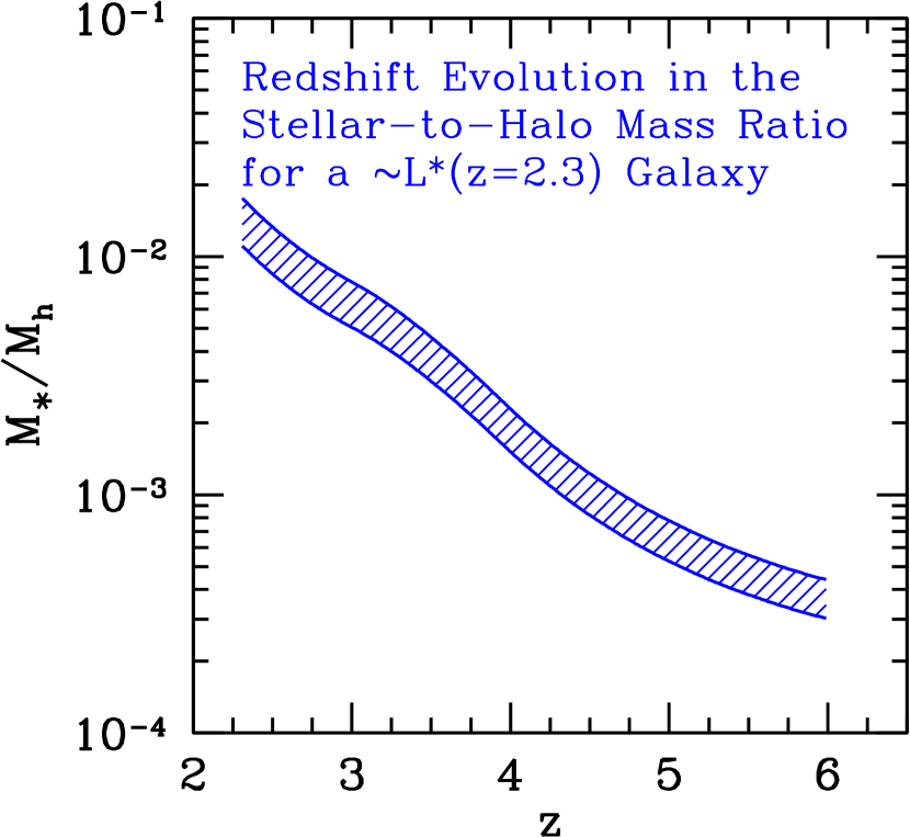
Figure 24.— Stellar-to-halo mass ratio as a function of redshift for a typical star-forming galaxy with a stellar mass at $z=2.3$ of $M_{\ast}^{z=2.3}=1.6\times 10^{10}$ M_⊙. Clustering results are used to estimate the corresponding average and median dark matter halo masses (Trainor & Steidel, in preparation). The stellar masses are evolved backwards in time using the same assumptions as in Figure 21. The median and average halo masses are evolved to higher redshift assuming the baryonic rate accretion formula specified by Equation 12.

8.4. Summary and Implications

In this section, we have discussed the typical star formation histories of high-redshift galaxies based on (a) an analysis of the median specific SFR as a function of stellar mass at $z\sim 2$, combined with (b) the observation that the specific SFR does not evolve strongly with redshift above $z\sim 4$, at least for galaxies for which such measurements have been obtained. These two pieces of evidence lead us to the conclusion that on average the SFRs of $z\gtrsim 2$ galaxies are likely rising monotonically with time. In this case, the “age” of the galaxy is an ill-defined quantity and in principle could be arbitrarily old depending on the normalization of the star formation history. As such, it is possible that a substantial fraction of the UV faint sub-$L^{\ast}$ galaxies at $z\gtrsim 4$ evolve into UV-bright galaxies (i.e., ones that we would spectroscopically confirm) at $z\sim 2$. Studies of the clustering properties of sub-L^∗ galaxies combined with halo abundance matching will undoubtedly help elucidate the probable progenitors of $z\sim 2$ galaxies.

We proceed to examine the evolution in gas masses and gas accretion rates implied by rising star formation histories assuming that the Kennicutt-Schmidt relation holds at high redshift. The results imply that the gas masses will increase with increasing SFR, and that the gas mass fraction will evolve more slowly than in a scenario in which galaxies are forming stars at a constant or declining rate. We find in general that mean cold gas fraction remains quite high at $\gtrsim 60\%$ at $z\gtrsim 4$. A further consequence of the slow evolution of gas mass fraction at $z\gtrsim 4$ is that the average gas phase metallicity may not evolve with time as strongly at $z\gtrsim 4$ relative to that observed at $z\lesssim 2$. This is because newly accreted gas will continually dilute the overall gas-phase metallicity. At face value, the fundamental metallicity relation (FMR) derived in Mannucci et al. (2010) implies an $\approx 0.5$ dex increase in mean oxygen abundance from $z=7$ to 4. However this relation has only been calibrated up to $z\sim 2.5$ and for larger SFRs at higher redshifts, than the SFRs considered here at $z\gtrsim 4$. Direct metallicity measurements for such high-redshift galaxies, while unobtainable at the present time, will prove crucial in connecting the metallicity evolution with that expected from the average increasing star formation rate between $z=7$ and 2.

At these early times, the net gas accretion rate exceeds the SFR by at least a factor of two, where the former is determined by relating the specific SFR to the cold gas mass via the Kennicutt (1998) relation. For the progenitors of typical star-forming galaxies in our $z\sim 2$ sample, the SFR eventually equals the net gas accretion rate around $z\sim 2-3$, at which point the gas fraction decreases below $50\%$. These results are consistent with measurements of the gas mass fractions of high-redshift galaxies, and the fact that such galaxies must be accreting substantial amounts of gas in order to sustain their SFRs.

We proceed to compare the gas accretion rates inferred from the specific SFR—combined with some assumption for the mass-loading factor of outflowing winds—with the accretion rates expected for the dark matter halos that are inferred from clustering to host galaxies in our sample. We find that the two methods of inferring gas accretion rates agree at $z\lesssim 3$, but they become increasingly divergent above $z\gtrsim 4$, such that less than one percent of the baryons accreted by a $\log[M_{\rm h}/{\rm M}_{\odot}]=11.2$ halo at $z\sim 6$ would end up in stars at that epoch. While several possibilities are discussed to explain this discrepancy, the results imply that star formation must have been extremely inefficient at early cosmic times.

9. CONCLUSIONS

We use a large spectroscopic sample of $L^{\ast}$ galaxies at redshifts $1.4\lesssim z\lesssim 3.7$, and a photometrically selected sample of fainter galaxies at the same redshifts, to constrain the average star formation history of typical star-forming galaxies between redshift $z=7$ and $z=2$. Our analysis takes advantage of rest-frame UV spectroscopy, and optical, ground-based near-IR, Hubble Space Telescope WFC3/IR, and Spitzer Space Telescope IRAC and MIPS $24$ $\mu$m imaging, in order to measure the stellar populations and dust obscured star formation of galaxies in our sample. We have taken into account a number of systematic effects in computing these quantities, including the contribution of line emission to the broadband photometry, dynamical time constraints on galaxy ages, and the stellar population dependence of the UV attenuation curve.

With these data, we perform detailed comparisons between SED-inferred SFRs (SFRs[SED]) and those computed by combining deep UV and MIPS $24$ $\mu$m data (SFRs[IR+UV]), for 302 spectroscopically confirmed galaxies at redshifts $1.5\lesssim z\lesssim 2.6$, where the MIPS $24$ $\mu$m observations are sensitive to the dust emission features at rest-frame $8$ $\mu$m; such comparisons allow us to rule out some simple star formation histories. The uncertainties in stellar masses and ages are discussed. We proceed to examine the correlation between SFR[IR+UV] and stellar mass, as well as SFR[SED] and stellar mass for a larger sample of 1959 spectroscopically confirmed galaxies, taking into account several systematic effects including Malmquist bias and differences in the conversion from near-IR luminosity to stellar mass. These results are extended to lower SFRs and stellar masses via a photometrically selected sample of 563 UV faint (${\cal R}>25.5$) galaxies over the same redshifts. This information is used to constrain the average star formation history of high-redshift galaxies, which in turn yields information on the gas mass evolution and gas mass accretion rates for galaxies of different stellar masses.

The main conclusions are:

• SED modeling that assumes exponentially declining star formation histories results in SFRs[SED] that are on average a factor of $5-10\times$ lower than SFRs[IR+UV]. On the other hand, modeling typical star-forming galaxies ($L_{\rm bol}\lesssim 10^{12}$ L_⊙; ages $\lesssim 100$ Myr) with constant or rising star formation histories and a Calzetti et al. (2000) attenuation curve results in SFRs[SED] that are in good agreement with SFRs[IR+UV]. This suggests that most $L^{\ast}$ galaxies at $z\sim 2-3$ did not follow a declining star formation history prior to the epoch at which they are observed. The traditional use of exponentially declining models to describe the star formation histories of high-redshift galaxies is called into question by the analysis presented in this paper.

• Assuming standard modeling assumptions (Calzetti et al. 2000 attenuation curve and no age constraint) results in SFRs[SED] that are systematically larger than SFRs[IR+UV] for galaxies inferred to have younger stellar populations ($\lesssim 100$ Myr). However, by building a coherent picture for the dust attenuation (SMC-like) and dynamical timescale of younger galaxies, we are able to reconcile the SFRs[SED] and SFRs[IR+UV] for such galaxies.

• Rising star formation histories yield stellar masses that are comparable to (and ages that are typically older than) those obtained for a constant star formation history, owing to the slower evolution in $M/L$ ratio for rising histories. More generally, the “age” of a galaxy is an ill-defined quantity for rising histories, as the observed $M/L$ ratio can be obtained by simultaneously varying the age of a galaxy and the normalization of its star formation history.

• The scatter in the $M/L$ ratios of galaxies at a given luminosity decreases at longer wavelengths. Nonetheless, the scatter, which is induced partly by the current star formation, is still relatively large ($0.20$ dex) at wavelengths where the stellar emission peaks ($\gtrsim 1$ $\mu$m). The luminosity dependence of the $M/L$ ratio at $1.1$ $\mu$m is partly a result of sampling a finite range of UV luminosity in a flux limited sample like ours, combined with the effects of dust obscuration. The systematic variation of the stellar mass versus near-IR magnitude relation with UV luminosity can result in biased measurements of the masses of UV-faint galaxies.

• Taking into account IRAC upper limits and the aforementioned UV luminosity dependence of the conversion between near-IR magnitude and stellar mass, we find a strong correlation between UV luminosity and stellar mass, even within the limited dynamic range of our spectroscopic sample. An IRAC stacking of photometrically selected UV faint galaxies to ${\cal R}\sim 27.0$ shows that this trend extends to UV faint galaxies. In particular, $0.1L^{\ast}$ galaxies at $z\sim 2$ have stellar masses that are a factor of $\approx 140\times$ smaller than those of the UV brightest ($\sim 5L^{\ast}$) galaxies in our sample.

• Combining the UV-faint data with our spectroscopic sample, and taking into account systematics in the calculation of stellar masses, we find a close to unity slope of the SFR-$M_{\ast}$ relation over $2.5$ orders of magnitude in stellar mass and $2.8$ orders of magnitude in SFR at $z\sim 2$. This relation implies that the specific SFR (SFR/$M_{\ast}$) is roughly constant for stellar masses $M_{\ast}\gtrsim 5\times 10^{8}$ M_⊙ and SFRs $\gtrsim 2$ M_⊙ yr^-1.

• The constant specific SFR with mass at $z\sim 2$, combined with the fact that this median SFR is similar to that found at $z\gtrsim 4$, implies that the SFRs must be increasing with (and roughly proportional to) the stellar mass. A constant star formation history would imply much larger specific SFRs at slightly higher redshifts, and such objects are not observed at those higher redshifts that are probed within our sample. If galaxies on average have SFRs that increase with cosmic time, then it suggests that the UV-bright galaxies observed at $z\sim 2-3$ had progenitors that would be detected as sub$-L^{\ast}$ galaxies in $z\gtrsim 4$ dropout samples.

• If we assume that the Kennicutt-Schmidt relation Kennicutt (1998) holds at high redshift, then an average rising star formation history implies a gas mass that increases with time and a gas mass fraction that evolves slowly at $z\gtrsim 4$. The specific SFRs at $z\gtrsim 2$ indicate a net cold gas accretion rate that outpaces the SFR at high redshift, until $z\sim 2-3$, when the SFR becomes comparable to the net cold gas accretion rate for typical star-forming galaxies. We have inferred the cold gas inflow rate from the net cold gas accretion rate with some assumption for the mass-loading factor of galactic outflows. The inflow rates derived in this manner diverge increasingly from the total gas inflow rates expected for the dark matter halos that host our galaxies (as inferred from clustering analysis; Trainor & Steidel, in prep.). At face value, the observations imply that less than one percent of the baryons accreted onto halos of mass $M_{\rm h}\simeq 1.6\times 10^{11}$ M_⊙ at $z\sim 6$ end up contributing to star formation at that epoch, thus highlighting the inefficiency of star formation even at early cosmic times when galaxies were growing rapidly.

There are two important points to make. First, taken together, the results of the SFR comparisons (Section 4), the near-unity slope of the SFR-$M^{\ast}$ relation, and the roughly similar specific SFRs at $z\gtrsim 2$, point to a picture in which the average SFRs of high-redshift galaxies increase with cosmic time. This behavior produces naturally the observed rise in the SFR density between $z=7$ and $z=4$ (Papovich et al., 2011). Second, an analysis of the specific SFRs indicate that these rising histories cannot be sustained indefinitely, and once the SFR exceeds the gas accretion rate, we expect the gas mass to decrease leading to an eventual decrease in SFR. However, our analysis underscores the fact that the net cold gas accretion inferred from the specific SFRs is only a small constituent of the total baryons accreted onto halos at $z\gtrsim 2$, and that in general star formation must have been very inefficient at early times.

We conclude by noting several future avenues of investigation to confirm more robustly our findings. We have emphasized a few of the biases (e.g., Malmquist bias and systematics in the conversion between near-IR luminosity and stellar mass) that are important for analyses of the SFR-$M^{\ast}$ (and specific SFR versus $M^{\ast}$) relations. The presence of a Malmquist bias, however, does not preclude the possibility of there being a real evolution in the SFR-$M^{\ast}$ relation at faint luminosities and low stellar masses. Hence, significant progress in evaluating possible evolution can be achieved with deep near-IR photometry (e.g., with Hubble Space Telescope’s WFC3/IR Camera) that in turn enables SED-fitting for individual UV-faint and low mass galaxies at high redshift. As emphasized above, there is a substantial dispersion in the star formation histories of individual galaxies; future deeper studies will enable us to quantify how the dispersion in SFRs may change as a function of $M^{\ast}$, particularly for UV-faint galaxies at $z\gtrsim 3$ which, from clustering studies, may exhibit a more episodic star formation history (Lee et al., 2011b). Further, as recently highlighted in Schaerer & de Barros (2009, 2010), the expected high equivalent width emission lines (e.g., H$\alpha$) of $z\gtrsim 4$ galaxies can result in factors of $2-3\times$ overestimates of their stellar masses from broadband SED fitting. Correcting for the presence of those emission lines may potentially result in a stronger evolution of specific SFR than has been found in other studies of $z\gtrsim 4$ galaxies (Stark et al., 2009; González et al., 2010; Bouwens et al., 2011a), and may partially resolve the discrepancies between current observations and numerical simulations regarding the evolution of specific SFRs at $z\gtrsim 4$ (e.g., Bouché et al. 2010; Dutton et al. 2010; Davé et al. 2011; Weinmann et al. 2011; Krumholz & Dekel 2011; see discussion in Bouwens et al. 2011a). The forthcoming deep near-IR imaging surveys, along with deep imaging and spectroscopic campaigns with the next generation of ground-based (TMT and GMT) and space-based facilities (JWST), promise substantial progress in understanding star formation and the buildup of stellar mass at early cosmic times.

Appendix A Conversion from UV Luminosity to Star Formation Rate

The conversion from UV luminosity to SFR will depend on the star formation history and age of a galaxy. This is illustrated in Figure 25, where we show the ratio of SFR to the $1700$ Å  luminosity as a function of age for different star formation histories. For ages $\lesssim 10$ Myr, the factor needed to convert a UV luminosity to a SFR is larger than the Madau et al. (1998); Kennicutt (1998) values because the ratio of O stars to B stars (both of which contribute significantly to the rest-frame $1700$ Å  luminosity) is larger than the equilibrium ratio reached after the B star main sequence lifetime of $\approx 100$ Myr. For older ages and exponentially declining star formation histories, the UV luminosity does not fall off as quickly with time as the SFR. In these cases, the ratio of O stars to B stars is lower than the case of continuous star formation (i.e., B stars will still contribute significantly to the UV luminosity even after the production rate of O stars declines). As the decay timescale $\tau_{\rm d}$ becomes larger and $t_{\rm age}/\tau_{\rm d}<1$, the conversion factor approaches that of the CSF history. Similarly, exponentially rising star formation histories have a conversion factor similar to, but slightly larger than, those obtained for a CSF history. In the rising histories, the ratio of O and B stars will stabilize to a value larger than in the CSF case since the SFR is continually increasing. The conversion factor for rising histories with larger $\tau_{\rm r}$ approaches the factor for a CSF case. For convenience, we have tabulated the form of the simple polynomial fits that describe the relationship between the ratio of SFR to $1700$ Å  luminosity as a function of age for the different star formation histories, assuming the latest CB11 models with a Salpeter IMF and solar metallicity (Table 6). In this parameterization, the conversion factor between UV luminosity and SFR is $C_{\rm UV}$, where

$$\frac{\rm SFR}{\rm M_{\odot}\,yr^{-1}}=C_{\rm UV}\times\frac{L_{1700}}{\rm erg\,s^{-1}\,Hz^{-1}},$$ (13)

and $C_{\rm UV}$ is approximated with a polynomial function of $\xi\equiv\log(t_{\rm age})$:

$$\log[C_{\rm UV}(\xi)]=\sum_{\rm i=0}^{\rm 5}a_{\rm i}[f(\xi)]^{\rm i}$$ (14)

where $f(\xi)=\xi$ or $1/\xi$, and the coefficients $a_{\rm i}$ are given in Table 6.

In the present context, changes in the conversion between UV luminosity and SFR will not significantly affect the bolometric SFRs for two reasons. First, as discussed in Section 4, the range of ages and star formation histories that are plausible at $z\sim 2$ rule out conversion factors that vary by more than $\approx 20\%$ from the equilibrium value. Secondly, the bolometric SFRs are less sensitive to changes in the UV-SFR conversion factor given that, for most of the galaxies in our sample, a significant fraction of the bolometric luminosity ($\simeq 80\%$) is emergent in the IR and not the UV (Reddy et al., 2006b, 2010). For simplicity, we assume the Kennicutt (1998) relation to convert UV luminosity to SFR, and we discuss in Section 4 how changing the conversion factor between these quantities affects (or does not significantly affect) our results.

Table 6Coefficients of Polynomial Fits to Logarithm of SFR/UV Conversion Factor, $\log[C_{\rm UV}]$

	$\tau$								Age Range
SFH	(Myr)	$f(\xi)$	$a_{0}$	$a_{1}$	$a_{2}$	$a_{3}$	$a_{4}$	$a_{5}$	(Myr)
Constant	$\infty$	$1/\xi$	-27.822	-0.969	2.511	-2.000	0.704	-0.089	$\geq 3$
Declining	10	$\xi$	-26.658	-1.662	0.568	-0.689	0.969	-0.395	3 – 255
	20	$\xi$	-26.433	-3.065	3.808	-3.592	1.936	-0.425	3 – 508
	50	$\xi$	-25.634	-7.271	11.088	-8.624	3.237	-0.471	3 – 1433
	100	$\xi$	-26.309	-3.416	3.665	-2.245	0.716	-0.093	3 – 905
	200	$1/\xi$	-28.906	3.768	-5.127	3.615	-1.176	0.140	3 – 1900
	500	$1/\xi$	-28.008	-0.238	1.404	-1.218	0.449	-0.059	3 – 4000
	1000	$1/\xi$	-27.889	-0.725	2.162	-1.764	0.630	-0.081	3 – 7000
	2000	$1/\xi$	-27.847	-0.888	2.409	-1.939	0.687	-0.088	$\geq 3$
	5000	$1/\xi$	-27.846	-0.855	2.311	-1.843	0.649	-0.082	$\geq 3$
Rising	100	$1/\xi$	-27.877	-0.049	0.390	-0.138	0.013	0.0002	$\geq 3$
	5000	$1/\xi$	-27.826	-0.921	2.401	-1.902	0.667	-0.085	$\geq 3$

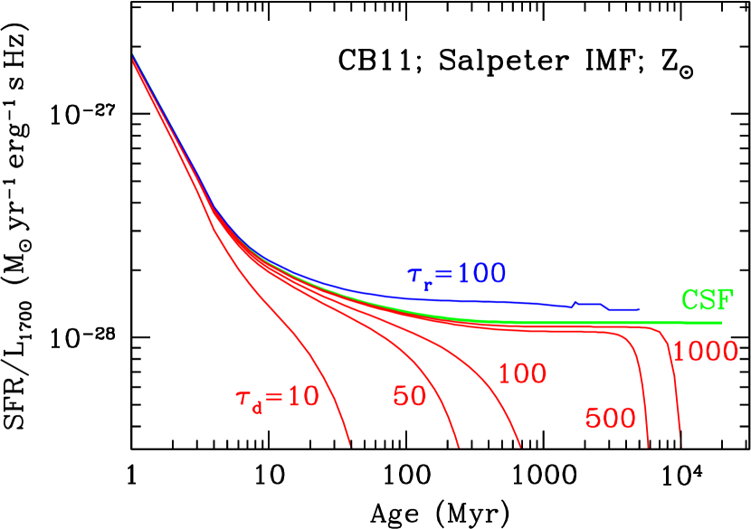
Figure 25.— Ratio of SFR to specific luminosity at 1700 Å  as a function of age for different star formation histories. The red curves show results for exponentially declining star formation histories with $\tau_{\rm d}=10$, $50$, $100$, $500$, and $1000$ Myr. The green curve shows the result for a CSF history. The blue curve shows the result for an exponentially rising star formation history with $\tau_{\rm r}=100$ Myr. Other rising histories with $\tau_{\rm r}>100$ Myr will be bracketed by the CSF and $\tau_{\rm r}=100$ Myr curves.

Appendix B The Effect of Malmquist Bias on the Mean SFR at a Given Stellar Mass

In this section, we explore the effect of Malmquist bias from a flux-limited sample on the mean SFRs in bins of stellar mass. To illustrate this bias, we simulated the effect of imposing a spectroscopic limit on a SFR versus stellar mass trend with an intrinsic slope of unity, and an rms dispersion of $0.38$ dex (based on the dispersion around the best-fit correlation shown in Figure 12). Because our sample is selected based on (unattenuated) UV emission, we first quantified the relationship between bolometric SFR and bolometric luminosity using the 302 galaxies in the MIPS $24$ $\mu$m sample. Reddy et al. (2010) give the relationship between bolometric and UV luminosity for this sample (with a mean redshift of $\langle z\rangle\simeq 2$) as

$$\log[L_{\rm UV}/{\rm L}_{\odot}]=\log[L_{\rm bol}/{\rm L}_{\odot}]-\log[{L_{\rm bol}}^{1/a}10^{-b/a}+1],$$ (15)

where $a=0.69\pm 0.03$ and $b=10.91\pm 0.04$. This relationship is redshift dependent, because the ratio of bolometric to UV luminosity at a given SFR decreases with increasing redshift (Reddy et al., 2006b, 2010). The mean trend between $L_{\rm UV}$ and SFR implies that galaxies with fainter UV luminosities also have on average lower bolometric SFRs (Reddy et al., 2010).

Second, to ensure a realistic weighting of points, we simulated a population of galaxies that has a Schechter (1976) distribution in bolometric SFR, with a characteristic SFR${}^{\ast}=30$ M_⊙ yr^-1 and faint-end slope $\alpha=-1.6$, based on the bolometric luminosity function at $z\sim 2$ (Reddy & Steidel, 2009). An $L_{\rm UV}$ was assigned to each galaxy based on its bolometric SFR and the observed relationship between SFR and $L_{\rm UV}$, as discussed above. Similarly, a stellar mass was assigned to each galaxy based on its SFR and the assumed intrinsic trend between SFR and $M_{\ast}$. In assigning $L_{\rm UV}$ and $M_{\ast}$, we randomly perturbed these values according to the dispersions measured in the SFR-$L_{\rm UV}$ ($\approx 0.5$ dex) and SFR-$M_{\ast}$ ($\approx 0.4$ dex) relations. The final step in the simulation was to remove all galaxies with $L_{\rm UV}\lesssim 10^{10}$ L_⊙, corresponding approximately to the spectroscopic limit at $z\sim 2$. The remaining galaxies are binned according their stellar masses. The average (or median) SFR for each bin is then calculated.

The results of this simple simulation are shown in Figure 26, which suggests that the UV flux limit will result in an artificial trend of increasing specific SFR ($\phi$) at low stellar masses, on an otherwise intrinsically flat relationship between $\phi$ and $M_{\ast}$. For example, in the lowest mass bin with $9.0\leq\log[M_{\ast}/{\rm M}_{\odot}]<9.5$, the recovered specific SFR is $\approx 3-4\times$ larger than the intrinsic value. Based on this simple simulation, and evidence that galaxies fainter than our spectroscopic limit have specific SFRs at $M_{\ast}\simeq 10^{9}$ M_⊙ that are lower than what we would have inferred had we relied on the SED fitting of the spectroscopic sample only (see the next section), we conclude that the true median specific star formation is lower than that measured for the lowest mass galaxies in our sample if these SFRs are also determined from SED fitting (Section 7). It is evident that the magnitude of this bias increases with the intrinsic scatter in the SFR-M_∗ relationship. More generally, these results highlight the importance of factoring in the UV luminosity limit of high-redshift dropout samples when determining mean SFRs (or specific SFRs) in bins of stellar mass. We show in Section 7 and Appendix C how this bias can also affect our determination of the near-IR luminosity dependence of the mass-to-light $M/L_{1.1\mu m}$ ratio. As such, the simulation discussed above does not tell the full story because we cannot directly measure the stellar masses of galaxies; the masses must be inferred from luminosity at a given wavelength (UV or near-IR), and therefore the position of the recovered galaxies along the stellar mass axis in the left panel of Figure 26 (and along both the $\phi$ and $M_{\ast}$ axes in the right panel) may not be accurate. In Appendix E we discuss the combined effects of these biases on determinations of the SFR-$M_{\ast}$ relation.

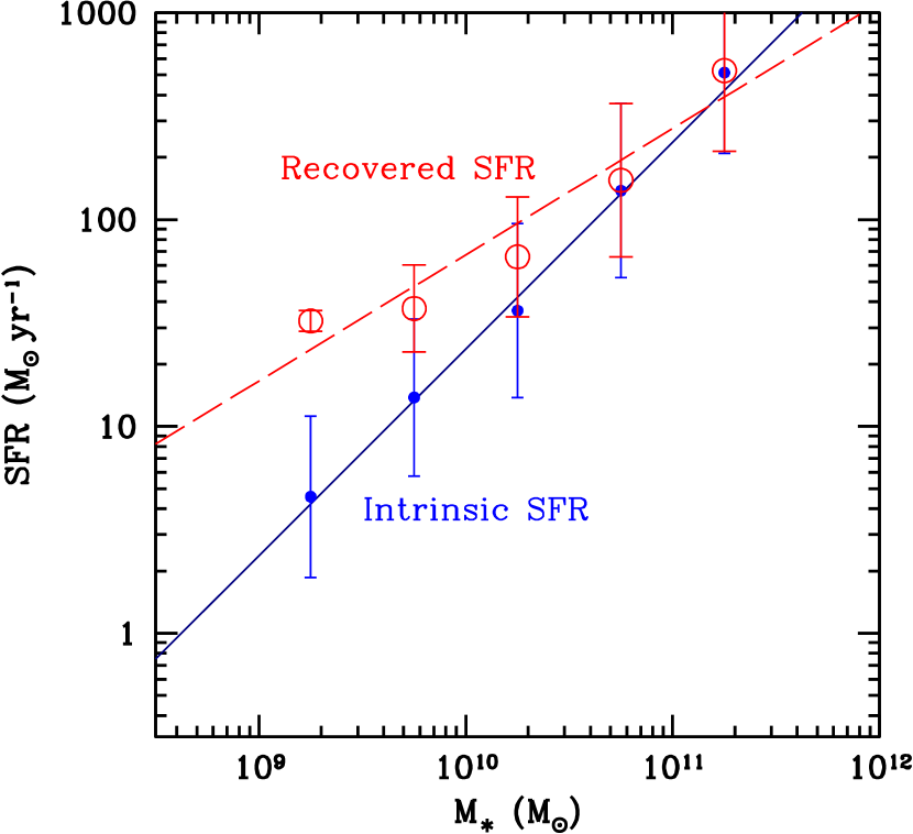
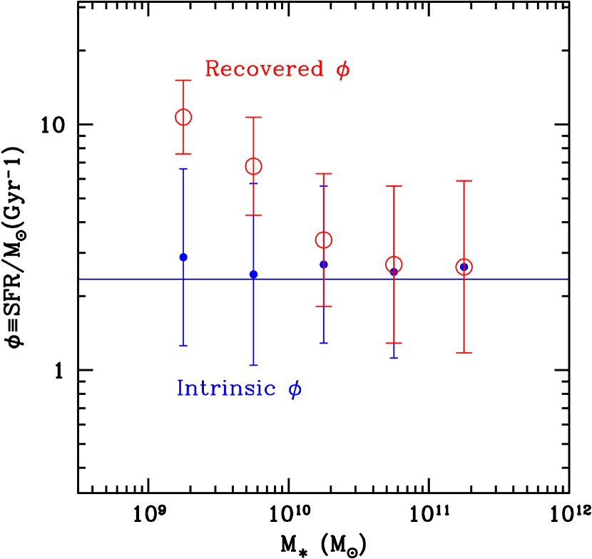
Figure 26.— Effects of Malmquist bias on the measurements of the SFR vs. stellar mass trend, and specific SFR $\phi$. The solid line indicates an assumed intrinsic specific SFR of $\phi\simeq 2.4\times 10^{-9}$ yr^-1. Accounting for the scatter between SFR and stellar mass results in recovered SFR and $\phi$ denoted by the solid blue symbols. The hollow red symbols indicate the measured SFR and $\phi$ when we fold in the scatter between SFR and UV luminosity, and impose a (spectroscopic) limit of $L_{\rm UV}=10^{10}$ L_⊙. Errorbars reflect the dispersion in SFR and $\phi$ in each bin of stellar mass.

Appendix C UV Dependence of the Relationship Between Stellar Mass and Near-IR Magnitude

C.1. Spectroscopic Sample

The Malmquist bias discussed in Appendix B can result in a slope between SFR and stellar mass that is artificially shallow compared to the intrinsic value. Similarly, there is a simple explanation for why this bias manifests itself onto the best-fit relation between stellar mass and near-IR luminosity as determined from a UV selected sample. Specifically, a flux-limited sample, like ours, will tend to miss galaxies with lower SFRs at a fixed (low) stellar mass (Section 6.4 and Appendix B). Therefore, the median near-IR magnitude in a given bin of stellar mass will be biased brighter because at a fixed stellar mass, galaxies with larger SFRs (and hence those that satisfy the UV flux limit) will have larger near-IR luminosities (i.e., current star formation will contribute at near-IR wavelengths).

This effect is demonstrated clearly in Figure 27. In particular, the large scatter in near-IR luminosity (or stellar mass) at a given UV luminosity (see Section 7.2.1), implies that there will be galaxies just below our flux limit that have similar stellar masses as galaxies that lie just above our flux limit. The result is that the median or average near-IR luminosity corresponding to a bin of stellar mass will be lower than what we would have predicted from a UV (bright) selected sample. Conversely, UV faint galaxies have a smaller contribution of current star formation to the near-IR light, and hence a given near-IR magnitude will correspond to a larger stellar mass for such galaxies. The inclusion of UV fainter galaxies results in a slope between $\log M_{\ast}$ and $M_{1.1}$ that is less negative than the one derived for a sample of UV-brighter galaxies (Figure 28. This has important implications for (1) determining the luminosity dependence of the mass-to-light ratio based on a UV/optical selected samples (e.g., Gonzalez et al. 2011; Lee et al. 2011b), and (2) translating the mean stellar mass found for galaxies of a given UV luminosity.

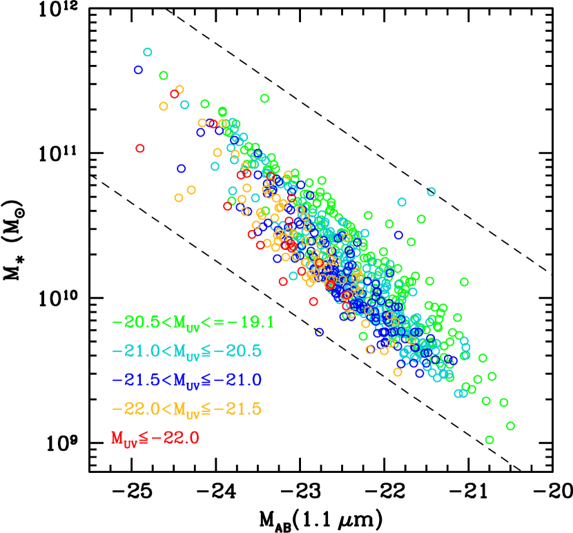
Figure 27.— Same as upper left panel of Figure 13, color coded by the absolute UV magnitude (at $1700$ AA), for galaxies directly detected in the channel 1 IRAC data. There is a clear trend between UV luminosity and the relation between stellar mass and near-IR magnitude, such that at a given stellar mass, UV-luminous galaxies exhibit brighter near-IR magnitudes.

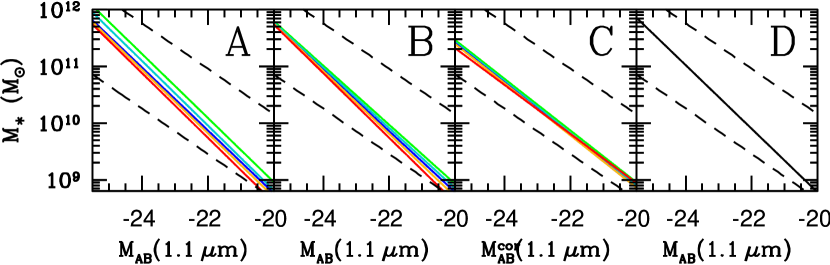
Figure 28.— Panel A: Best-fit linear relations between stellar mass and near-IR magnitude for galaxies in the UV magnitude bins indicated in Figure 27. Panel B: Best-fit linear relations between stellar mass and near-IR magnitude for galaxies brighter than the faint magnitude limit of each of the UV magnitude bins indicated in Figure 27. Panel C: Same as Panel B, where we have corrected the near-IR magnitude for the affects of dust extinction, assuming the best-fit $E(B-V)$ and either the Calzetti et al. (2000) or SMC attenuation curve depending on whether the galaxy is “young” (Section 5). Panel D: Best-fit linear relation between stellar mass and near-IR magnitude (uncorrected for dust) for all galaxies with $M_{1.1}<-22.0$. In all panels, the dotted lines indicate the maximum and minimum mass-to-light ratio found in the sample.

To illustrate these points, the best-fit linear relation between log stellar mass and near-IR magnitude ($\log M_{\ast}-M_{1.1}$) for galaxies in the different UV luminosity bins denoted in Figure 27 are shown in Panel A of Figure 28. Panel B indicates the best-fit relations when we fit for all galaxies above the faint magnitude limits of the bins in UV luminosity. As we add UV faint galaxies, the best-fit slope between stellar mass and near-IR magnitude becomes shallower (less steep). The slope of the $\log M_{\ast}-M_{1.1}$ relation can also be affected by dust, because galaxies with larger stellar mass have on average larger SFRs and hence larger dust obscuration. Hence, the Panel C of Figure 28 shows that correcting the near-IR magnitudes for the effects of dust attenuation results in a slope of the $\log M_{\ast}-M_{1.1}$ relation that is very close to $0.4$, implying a dust-corrected $M/L$ ratio at $1.1$ $\mu$m that is only very weakly dependent on near-IR luminosity.

Finally, Figure 27 suggests that our UV selected galaxies sample approximately the full range of stellar masses down to $M_{1.1}\simeq-22.0$ Therefore, Panel D of Figure 28 indicates the best-fit correlation between near-IR magnitude (uncorrected for dust) and stellar mass for all galaxies in our sample with $M_{1.1}<-22$ The best-fit linear relations and the rms dispersion of the data about these linear fits are tabulated in Table 7. The important point demonstrated in Figures 27 and 28 is that the systematic biases introduced by virtue of having a flux limited sample, combined with the effects of dust attenuation, can easily influence our interpretation of the presence of a luminosity dependence of the $M/L$ ratio.

Table 7Best-Fit Linear Relations Between Stellar Mass and Near-IR ($1.1$ $\mu$m) Magnitude

Panel	$M_{\rm UV}$ or $M_{1.1}$ Range	$\log[M_{\ast}/{\rm M}_{\odot}]=$	RMS
A	$-20.5<M_{\rm UV}\leq-19.1$	$-(0.56\pm 0.02)M_{1.1}-(2.33\pm 0.39)$	0.19
	$-21.0<M_{\rm UV}\leq-20.5$	$-(0.57\pm 0.02)M_{1.1}-(2.58\pm 0.39)$	0.17
	$-21.5<M_{\rm UV}\leq-21.0$	$-(0.55\pm 0.02)M_{1.1}-(2.32\pm 0.46)$	0.16
	$-22.0<M_{\rm UV}\leq-21.5$	$-(0.56\pm 0.03)M_{1.1}-(2.51\pm 0.67)$	0.16
	$M_{\rm UV}\leq 22.0$	$-(0.57\pm 0.07)M_{1.1}-(2.80\pm 1.64)$	0.19
B	$M_{\rm UV}\leq-19.1$	$-(0.52\pm 0.01)M_{1.1}-(1.49\pm 0.24)$	0.20
	$M_{\rm UV}\leq-20.5$	$-(0.53\pm 0.01)M_{1.1}-(1.75\pm 0.26)$	0.18
	$M_{\rm UV}\leq-21.0$	$-(0.54\pm 0.02)M_{1.1}-(1.98\pm 0.35)$	0.17
	$M_{\rm UV}\leq-21.5$	$-(0.55\pm 0.03)M_{1.1}-(2.36\pm 0.62)$	0.17
C	$M_{\rm UV}\leq-19.1$	$-(0.46\pm 0.01)M^{\rm cor}_{1.1}-(0.15\pm 0.23)$	0.22
	$M_{\rm UV}\leq-20.5$	$-(0.46\pm 0.01)M^{\rm cor}_{1.1}-(0.26\pm 0.27)$	0.20
	$M_{\rm UV}\leq-21.0$	$-(0.46\pm 0.02)M^{\rm cor}_{1.1}-(0.37\pm 0.36)$	0.19
	$M_{\rm UV}\leq-21.5$	$-(0.45\pm 0.03)M^{\rm cor}_{1.1}-(0.32\pm 0.64)$	0.20
	$M_{\rm UV}\leq-22.0$	$-(0.43\pm 0.07)M^{\rm cor}_{1.1}-(0.31\pm 1.67)$	0.24
D	$M_{1.1}<-22.0$	$-(0.56\pm 0.09)M_{1.1}-(2.42\pm 1.94)$	0.12

C.2. UV Faint Sample

We have several options for inferring the stellar masses of UV faint galaxies that lie below our spectroscopic limit. One possibility is to simple assume the same relationship between near-IR magnitude and stellar mass as was found for the faintest UV luminosity bin in our spectroscopic sample. A second option is to attempt to fit for the average SED of these UV faint galaxies. This option is beyond the scope of this paper and is not explored further. A third option is to extrapolate UV luminosity dependence of the $\log M_{\ast}-M_{1.1}$ relation to UV faint galaxies. While the marginalized uncertainties in the slope and intercept of the $\log M_{\ast}-M_{1.1,0.9}$ relations for the different UV luminosity bins in the spectroscopic sample suggest very little evolution (Table 7), there is some indication that the relation systematically shifts in normalization towards higher masses at fainter UV-luminosities (Panel A of Figure 28), as would be expected if these UV faint galaxies have a lower contribution of current star formation to the near-IR magnitude (see discussion above and in Section 7.2.1). By extrapolation from the UV-bright bins, the intercepts of the $\log M_{\ast}-M_{1.1,0.9}$ relation are computed as $b=0.14M_{\rm UV}+0.55$. The slope is kept fixed at $\delta\log[M_{\ast}/{\rm M}_{\odot}]/\delta M_{1.1,0.9}=-0.56$ (similar to that found for the more UV luminous bins). Converting the stacked IRAC channel 1 magnitudes listed in Table 5, we find that the median stellar masses obtained in this way are $\log[M_{\ast}/{\rm M}_{\odot}]=9.02$ and $8.71$ for the two UV faint bins at $z\sim 2$. Similarly, we find $\log[M_{\ast}/{\rm M}_{\odot}]=9.19$ and $9.12$ for the two faint bins at $z\sim 3$. The uncertainties in these stellar masses include: (1) measurement uncertainties in the stacked IRAC fluxes, (2) statistical uncertainties in the fit between near-IR magnitude and stellar mass, and (3) systematic uncertainties in the relation used to convert between near-IR magnitude and stellar mass (e.g., arising from the use of other of the other options mentioned above). Combining the errors from these effects in quadrature results in stellar mass uncertainties of $\approx 0.15-0.29$ dex.

Appendix D IRAC Stacking Method

As noted in Section 3, we modeled the stellar populations only for those galaxies that were directly detected at wavelengths longward of rest-frame $4000$ Å  to ensure that robust mass determinations included information from the age-sensitive Balmer and $4000$ Å  breaks. However, a substantial fraction of galaxies in the spectroscopic sample are undetected at these longer wavelengths, particularly those with fainter UV luminosities, as demonstrated in Figure 15. For an unbiased view of the mass distribution, we stacked the IRAC data in bins of UV luminosity.

Our stacking analysis proceeded as follows. Cutouts around each galaxy in our sample were assembled from the IRAC images. We included in the stack any galaxy that (1) does not show evidence of AGN, (2) has a spectroscopic redshift in the range $1.4\leq z<3.7$, (3) has an IRAC exposure time of more than 7200 sec, (4) is not blended with any nearby neighbor, and (5) lies more than $2\farcs 4$ away from any nearby source as identified in higher resolution optical and near-IR data. The cutouts were then median combined, though average combination yielded similar results. Given the field-dependent variation of the IRAC PSF, we constructed a “stacked PSF” made in exactly the same way as the regular stack — i.e., for each galaxy that went into the stack, we also stacked the PSF appropriate for the field in which that galaxy lies. Photometry on the stacked image was measured by fitting the stacked PSF to the stacked IRAC signal. Table 8 summarizes the stacked photometry, converted to absolute magnitudes based on the median redshifts of the objects that went into the stacks.

Table 8Stacked IRAC Magnitudes for Spectroscopic Sample

Redshift Interval	M(1700Å) Range	3.6 $\mu$m	4.5 $\mu$m	5.8 $\mu$m	8.0 $\mu$m
$1.4\leq z<2.7$	-22.5     -22.0	$-23.92\pm 0.13$ (4)	…	…	$-24.06\pm 0.16$ (2)
	-22.0     -21.5	$-22.87\pm 0.21$ (28)	$-22.93\pm 0.19$ (26)	$-23.19\pm 0.20$ (12)	$-22.95\pm 0.20$ (22)
	-21.5     -21.0	$-22.20\pm 0.17$ (72)	$-22.27\pm 0.17$ (48)	$-22.41\pm 0.19$ (31)	$-22.25\pm 0.21$ (55)
	-21.0     -20.5	$-21.95\pm 0.20$ (192)	$-21.85\pm 0.19$ (138)	$-22.14\pm 0.20$ (78)	$-21.78\pm 0.23$ (147)
	-20.5     -20.0	$-21.61\pm 0.19$ (199)	$-21.79\pm 0.20$ (180)	$-21.99\pm 0.21$ (93)	$-21.68\pm 0.22$ (189)
	-20.0     -19.5	$-21.14\pm 0.21$ (113)	$-21.15\pm 0.19$ (79)	$-21.35\pm 0.26$ (39)	$-21.02\pm 0.29$ (93)
	-19.5     -19.0	$-20.85\pm 0.21$ (22)	$-20.96\pm 0.26$ (22)	…	…
$2.7\leq z<3.7$	-23.0     -22.5	$-23.51\pm 0.27$ (2)	…	…	…
	-22.5     -22.0	$-22.45\pm 0.13$ (13)	$-23.18\pm 0.12$ (6)	$-23.06\pm 0.32$ (6)	$-23.54\pm 0.21$ (6)
	-22.0     -21.5	$-22.35\pm 0.12$ (45)	$-22.49\pm 0.13$ (34)	$-22.32\pm 0.25$ (21)	$-22.57\pm 0.16$ (34)
	-21.5     -21.0	$-21.83\pm 0.13$ (104)	$-21.83\pm 0.12$ (78)	$-21.87\pm 0.18$ (52)	$-21.99\pm 0.19$ (79)
	-21.0     -20.5	$-21.37\pm 0.12$ (108)	$-21.49\pm 0.13$ (84)	$-21.48\pm 0.25$ (65)	$-21.13\pm 0.30$ (81)
	-20.5     -20.0	$-20.97\pm 0.16$ (68)	$-21.12\pm 0.12$ (57)	…	…

Appendix E Combined Effect of Biases on the SFR-$M_{\ast}$ Relation

In this section, we discuss the combined affect of the biases discussed in Appendices B and C. To recap, there is Malmquist bias of selecting galaxies with larger star formation rates at a given stellar mass in a flux limited sample. Second, there is a bias introduced by the conversion that one used to convert near-IR luminosity to stellar mass. To investigate jointly these effects, we built upon the simulations discussed in Appendix B. For each galaxy in the simulation, we assigned it a near-IR magnitude $M_{1.1}$ based on its UV magnitude, using the correlation between these two quantities, taking into account upper limits in near-IR magnitude with the EM parametric estimator (Figure 14):

$$M_{1.1}=0.90M_{1700}-3.41$$ (16)

with a dispersion of 1 dex. This near-IR magnitude was then converted to a “measured” stellar mass, $M^{\rm meas}_{\ast}$, using three different options. In the first option, $M^{\rm meas}_{\ast}$ is estimated for each galaxy using the $\log M_{\ast}-M_{1.1}$ relation appropriate for the UV luminosity of that galaxy (Panel A of Figure 28, and Table 7), and assuming that galaxies fainter than $M_{1700}=-19.1$ follow the relation for galaxies with $-20.5<M_{1700}\leq-19.1$ . In the second option, $M^{\rm meas}_{\ast}$ is estimated for each galaxy using the $\log M_{\ast}-M_{1.1}$ relation found for all galaxies in our spectroscopic sample with $M_{1700}\leq-19.1$ (Panel B of Figure 28, and Table 7). In the third option, $M^{\rm meas}_{\ast}$ is estimated for each galaxy using a $\log M_{\ast}-M_{1.1}$ relation with a fixed slope of $\delta\log[M_{\ast}/{\rm M}_{\odot}]/\delta M_{1.1}=-0.56$ and an intercept that evolves with $M_{1700}$ (see Appendix C).

The comparison between the simulated ($M^{\rm sim}_{\ast}$) and measured stellar masses is shown in Panel (a) of Figure 29. For the first two options, there is a tendency to underestimate $M^{\rm sim}_{\ast}$ because we attribute too large a fraction of the near-IR light to star formation rather than stellar mass. With the third option, we obtain a reasonable agreement between $M^{\rm sim}_{\ast}$ and $M^{\rm meas}_{\ast}$. Applying a magnitude cut results in an artificial offset between $M^{\rm meas}_{\ast}$ and $M^{\rm sim}_{\ast}$ because fainter galaxies will be excluded by the magnitude limit, leaving only brighter (and more massive simulated) galaxies in the bins of $M^{\rm meas}_{\ast}$. The middle row shows the recovered SFR-$M_{\ast}$ relation, where galaxies are binned by $M^{\rm meas}_{\ast}$. Because options 1 and 2 result in an underestimation of stellar mass, there is tendency to predict a shallower slope of the SFR-$M_{\ast}$ relation. Introducing a ${\cal R}<27.0$ limit then causes us to overestimate the median SFR in bins of $M^{\rm meas}_{\ast}$, due to Malmquist bias (Appendix B). Finally, the bottom row shows the results when binning by SFR, instead of $M^{\rm meas}_{\ast}$. In this case, as expected, the Malmquist bias is less noticeable, because at a given low SFR (or faint UV luminosity) we can probe the full range of stellar mass, or at least quantify the average stellar mass using stacking analyses (Figure 14 and Appendix D). The results from the simulations underscore how the obvious Malmquist bias and the subtler bias arising from the conversion between near-IR light and stellar mass can affect our interpretation of the SFR-$M_{\ast}$ relation. In practice, estimating the SFR-$M_{\ast}$ relation in bins of SFR may yield more accurate results that are largely immune to the effects of Malmquist bias, though one will still have to account for systematics in the conversion between near-IR light and stellar mass, particularly if SED-fitting for all the objects in a sample is not an option. In our case, for the UV faint samples, we determined median stellar masses in bins of UV luminosity, which roughly translates into bins of SFR, so our estimates should be largely unaffected by the Malmquist bias discussed above.

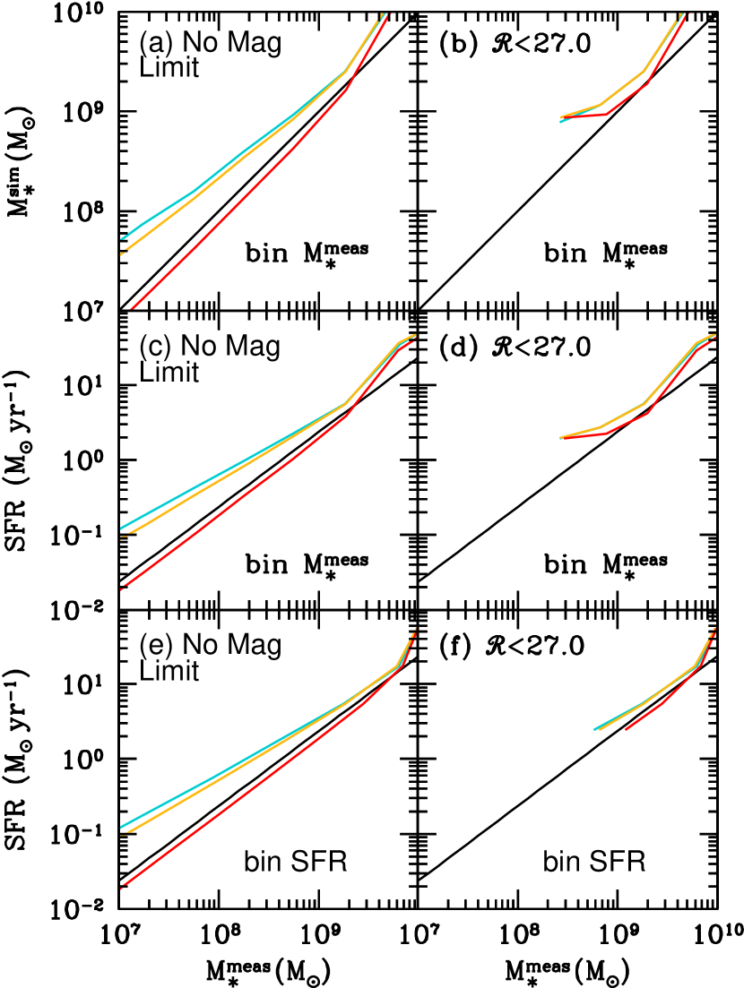
Figure 29.— Comparison between simulated (black lines) and measured stellar mass ($M^{\rm meas}_{\ast}$), binned by the latter, for galaxies in the full simulated sample (top row, panel a) and those brighter than ${\cal R}=27.0$ (top row, panel b). The cyan, orange, and red lines assume options one, two, and three described in the text for converting near-IR magnitude to stellar mass. The middle row indicates the same for the median input SFR in bins of $M^{\rm meas}_{\ast}$. The bottom row indicates the same, except binned in terms of SFR.

References

- Adelberger et al. (1998) Adelberger, K. L., Steidel, C. C., Giavalisco, M., et al. 1998, ApJ, 505, 18
- Adelberger et al. (2004) Adelberger, K. L., Steidel, C. C., Shapley, A. E., et al. 2004, ApJ, 607, 226
- Bell & de Jong (2000) Bell, E. F. & de Jong, R. S. 2000, MNRAS, 312, 497
- Bertin & Arnouts (1996) Bertin, E. & Arnouts, S. 1996, A&AS, 117, 393
- Bouché et al. (2010) Bouché, N., Dekel, A., Genzel, R., et al. 2010, ApJ, 718, 1001
- Bouwens et al. (2009) Bouwens, R. J., Illingworth, G. D., Franx, M., et al. 2009, ApJ, 705, 936
- Bouwens et al. (2011a) Bouwens, R. J., Illingworth, G. D., Oesch, P. A., et al. 2011a, ArXiv e-prints
- Bouwens et al. (2011b) Bouwens, R. J., Illingworth, G. D., Oesch, P. A., et al. 2011b, ApJ, 737, 90
- Brinchmann et al. (2004) Brinchmann, J., Charlot, S., White, S. D. M., et al. 2004, MNRAS, 351, 1151
- Bruzual & Charlot (2003) Bruzual, G. & Charlot, S. 2003, MNRAS, 344, 1000
- Calzetti et al. (2000) Calzetti, D., Armus, L., Bohlin, R. C., et al. 2000, ApJ, 533, 682
- Conroy et al. (2008) Conroy, C., Shapley, A. E., Tinker, J. L., Santos, M. R., & Lemson, G. 2008, ApJ, 679, 1192
- Daddi et al. (2010) Daddi, E., Bournaud, F., Walter, F., et al. 2010, ApJ, 713, 686
- Daddi et al. (2007) Daddi, E., Dickinson, M., Morrison, G., et al. 2007, ApJ, 670, 156
- Davé et al. (2011) Davé, R., Oppenheimer, B. D., & Finlator, K. 2011, MNRAS, 415, 11
- Dekel et al. (2009) Dekel, A., Birnboim, Y., Engel, G., et al. 2009, Nature, 457, 451
- Dutton et al. (2010) Dutton, A. A., van den Bosch, F. C., & Dekel, A. 2010, MNRAS, 405, 1690
- Erb (2008) Erb, D. K. 2008, ApJ, 674, 151
- Erb et al. (2006a) Erb, D. K., Steidel, C. C., Shapley, A. E., et al. 2006a, ApJ, 647, 128
- Erb et al. (2006b) —. 2006b, ApJ, 646, 107
- Faucher-Giguère et al. (2011) Faucher-Giguère, C.-A., Kereš, D., & Ma, C.-P. 2011, MNRAS, 1399
- Ferguson et al. (2004) Ferguson, H. C., Dickinson, M., Giavalisco, M., et al. 2004, ApJ, 600, L107
- Finlator & Davé (2008) Finlator, K. & Davé, R. 2008, MNRAS, 385, 2181
- Finlator et al. (2011) Finlator, K., Oppenheimer, B. D., & Davé, R. 2011, MNRAS, 410, 1703
- Genzel et al. (2010) Genzel, R., Tacconi, L. J., Gracia-Carpio, J., et al. 2010, MNRAS, 407, 2091
- Goldader et al. (2002) Goldader, J. D., Meurer, G., Heckman, T. M., et al. 2002, ApJ, 568, 651
- Gonzalez et al. (2011) Gonzalez, V., Bouwens, R., Labbe, I., et al. 2011, ArXiv e-prints
- González et al. (2010) González, V., Labbé, I., Bouwens, R. J., et al. 2010, ApJ, 713, 115
- Gordon et al. (2001) Gordon, K. D., Misselt, K. A., Witt, A. N., & Clayton, G. C. 2001, ApJ, 551, 269
- Isobe et al. (1986) Isobe, T., Feigelson, E. D., & Nelson, P. I. 1986, ApJ, 306, 490
- Kennicutt (1998) Kennicutt, R. C. 1998, ARA&A, 36, 189
- Koekemoer et al. (2002) Koekemoer, A. M., Fruchter, A. S., Hook, R. N., & Hack, W. 2002, in The 2002 HST Calibration Workshop : Hubble after the Installation of the ACS and the NICMOS Cooling System, ed. S. Arribas, A. Koekemoer, & B. Whitmore, 337–+
- Komatsu et al. (2009) Komatsu, E., Dunkley, J., Nolta, M. R., et al. 2009, ApJS, 180, 330
- Kriek et al. (2010) Kriek, M., Labbé, I., Conroy, C., et al. 2010, ApJ, 722, L64
- Krumholz & Dekel (2011) Krumholz, M. R. & Dekel, A. 2011, ArXiv e-prints
- Law et al. (2009) Law, D. R., Steidel, C. C., Erb, D. K., et al. 2009, ApJ, 697, 2057
- Law et al. (2012) Law, D. R., Steidel, C. C., Shapley, A. E., et al. 2012, ApJ, 745, 85
- Lee et al. (2011a) Lee, K.-S., Dey, A., Reddy, N., et al. 2011a, ApJ, 733, 99
- Lee et al. (2011b) Lee, K.-S., Ferguson, H. C., Wiklind, T., et al. 2011b, ArXiv e-prints
- Lee et al. (2009) Lee, K.-S., Giavalisco, M., Conroy, C., et al. 2009, ApJ, 695, 368
- Madau (1995) Madau, P. 1995, ApJ, 441, 18
- Madau et al. (1998) Madau, P., Pozzetti, L., & Dickinson, M. 1998, ApJ, 498, 106
- Magdis et al. (2010) Magdis, G. E., Elbaz, D., Daddi, E., et al. 2010, ApJ, 714, 1740
- Magnelli et al. (2011) Magnelli, B., Elbaz, D., Chary, R. R., et al. 2011, A&A, 528, A35+
- Makovoz & Marleau (2005) Makovoz, D. & Marleau, F. R. 2005, astro-ph/0507007
- Mannucci et al. (2010) Mannucci, F., Cresci, G., Maiolino, R., Marconi, A., & Gnerucci, A. 2010, MNRAS, 408, 2115
- Maraston et al. (2006) Maraston, C., Daddi, E., Renzini, A., et al. 2006, ApJ, 652, 85
- Maraston et al. (2010) Maraston, C., Pforr, J., Renzini, A., et al. 2010, MNRAS, 407, 830
- Marchesini et al. (2009) Marchesini, D., van Dokkum, P. G., Förster Schreiber, N. M., et al. 2009, ApJ, 701, 1765
- Marigo & Girardi (2007) Marigo, P. & Girardi, L. 2007, A&A, 469, 239
- Melbourne et al. (2012) Melbourne, J., Williams, B. F., Dalcanton, J. J., et al. 2012, ApJ, 748, 47
- Meurer et al. (1999) Meurer, G. R., Heckman, T. M., & Calzetti, D. 1999, ApJ, 521, 64
- Misselt et al. (2001) Misselt, K. A., Gordon, K. D., Clayton, G. C., & Wolff, M. J. 2001, ApJ, 551, 277
- Moster et al. (2010) Moster, B. P., Somerville, R. S., Maulbetsch, C., et al. 2010, ApJ, 710, 903
- Muzzin et al. (2009) Muzzin, A., Marchesini, D., van Dokkum, P. G., et al. 2009, ApJ, 701, 1839
- Nagamine et al. (2000) Nagamine, K., Cen, R., & Ostriker, J. P. 2000, ApJ, 541, 25
- Nandra et al. (2002) Nandra, K., Mushotzky, R. F., Arnaud, K., et al. 2002, ApJ, 576, 625
- Noeske et al. (2007) Noeske, K. G., Weiner, B. J., Faber, S. M., et al. 2007, ApJ, 660, L43
- Noll et al. (2009) Noll, S., Burgarella, D., Giovannoli, E., et al. 2009, A&A, 507, 1793
- Oesch et al. (2010) Oesch, P. A., Bouwens, R. J., Carollo, C. M., et al. 2010, ApJ, 709, L21
- Oke et al. (1995) Oke, J. B., Cohen, J. G., Carr, M., et al. 1995, PASP, 107, 375
- Oppenheimer & Davé (2006) Oppenheimer, B. D. & Davé, R. 2006, MNRAS, 373, 1265
- Oppenheimer & Davé (2008) —. 2008, MNRAS, 642
- Oppenheimer et al. (2011) Oppenheimer, B. D., Davé, R., Katz, N., Kollmeier, J. A., & Weinberg, D. H. 2011, MNRAS, 2017
- Pannella et al. (2009) Pannella, M., Carilli, C. L., Daddi, E., et al. 2009, ApJ, 698, L116
- Papovich et al. (2001) Papovich, C., Dickinson, M., & Ferguson, H. C. 2001, ApJ, 559, 620
- Papovich et al. (2011) Papovich, C., Finkelstein, S. L., Ferguson, H. C., Lotz, J. M., & Giavalisco, M. 2011, MNRAS, 412, 1123
- Papovich et al. (2006) Papovich, C., Moustakas, L. A., Dickinson, M., et al. 2006, ApJ, 640, 92
- Pettini et al. (2002) Pettini, M., Rix, S. A., Steidel, C. C., et al. 2002, ApJ, 569, 742
- Quider et al. (2009) Quider, A. M., Pettini, M., Shapley, A. E., & Steidel, C. C. 2009, MNRAS, 398, 1263
- Reddy et al. (2012) Reddy, N., Dickinson, M., Elbaz, et al. 2012, ApJ, 744, 154
- Reddy et al. (2010) Reddy, N. A., Erb, D. K., Pettini, M., Steidel, C. C., & Shapley, A. E. 2010, ApJ, 712, 1070
- Reddy & Steidel (2004) Reddy, N. A. & Steidel, C. C. 2004, ApJ, 603, L13
- Reddy & Steidel (2009) —. 2009, ApJ, 692, 778
- Reddy et al. (2006a) Reddy, N. A., Steidel, C. C., Erb, D. K., Shapley, A. E., & Pettini, M. 2006a, ApJ, 653, 1004
- Reddy et al. (2006b) Reddy, N. A., Steidel, C. C., Fadda, D., et al. 2006b, ApJ, 644, 792
- Reddy et al. (2008) Reddy, N. A., Steidel, C. C., Pettini, M., et al. 2008, ApJS, 175, 48
- Renzini (2009) Renzini, A. 2009, MNRAS, 398, L58
- Riechers et al. (2010) Riechers, D. A., Carilli, C. L., Walter, F., & Momjian, E. 2010, ApJ, 724, L153
- Salpeter (1955) Salpeter, E. E. 1955, ApJ, 121, 161
- Sawicki (2011) Sawicki, M. 2011, ArXiv e-prints
- Sawicki & Yee (1998) Sawicki, M. & Yee, H. K. C. 1998, AJ, 115, 1329
- Schaerer & de Barros (2009) Schaerer, D. & de Barros, S. 2009, A&A, 502, 423
- Schaerer & de Barros (2010) —. 2010, A&A, 515, A73
- Schechter (1976) Schechter, P. 1976, ApJ, 203, 297
- Schmidt (1959) Schmidt, M. 1959, ApJ, 129, 243
- Seibert et al. (2002) Seibert, M., Heckman, T. M., & Meurer, G. R. 2002, AJ, 124, 46
- Shapley et al. (2001) Shapley, A. E., Steidel, C. C., Adelberger, K. L., et al. 2001, ApJ, 562, 95
- Shapley et al. (2005) Shapley, A. E., Steidel, C. C., Erb, D. K., et al. 2005, ApJ, 626, 698
- Shapley et al. (2003) Shapley, A. E., Steidel, C. C., Pettini, M., & Adelberger, K. L. 2003, ApJ, 588, 65
- Stark et al. (2009) Stark, D. P., Ellis, R. S., Bunker, A., et al. 2009, ApJ, 697, 1493
- Steidel et al. (2003) Steidel, C. C., Adelberger, K. L., Shapley, A. E., et al. 2003, ApJ, 592, 728
- Steidel et al. (2004) Steidel, C. C., Shapley, A. E., Pettini, M., et al. 2004, ApJ, 604, 534
- Tacconi et al. (2010) Tacconi, L. J., Genzel, R., Neri, R., et al. 2010, Nature, 463, 781
- Tinsley (1980) Tinsley, B. M. 1980, Fund. Cosmic Phys., 5, 287
- van der Wel et al. (2011) van der Wel, A., Straughn, A. N., Rix, H.-W., et al. 2011, ApJ, 742, 111
- van Dokkum et al. (2006) van Dokkum, P. G., Quadri, R., Marchesini, D., et al. 2006, ApJ, 638, L59
- Weinmann et al. (2011) Weinmann, S. M., Neistein, E., & Dekel, A. 2011, MNRAS, 1463
- Williams et al. (2010) Williams, B. F., Dalcanton, J. J., Stilp, A., et al. 2010, ApJ, 709, 135
- Wuyts et al. (2011) Wuyts, S., Forster Schreiber, N. M., Lutz, D., et al. 2011, ArXiv e-prints