Entanglement amplification of fermionic systems in an accelerated frame

Abstract

In this article we present an analysis to derive physical results in the entanglement amplification of fermonic systems in the relativistic regime, that is, beyond the single-mode approximation. This leads a recent work in [M. Montero and E. Martín-Martínez, JEHP 07 (2011) 006] to a physical result, and solidifies that phenomenon of entanglement amplification can actually happen in the relativistic regime.

I Introduction

Entanglement, that is, correlations existing in multipartite quantum systems, is an essential feature to describe information processing of physical systems in the most fundamental level of physics. It is known that, none of correlation measures which have been employed to describe correlations of classical systems suffices to describe entanglement. Then, a number of measures to quantify entanglement of quantum systems in the non-relativistic regime have been developed, for instance, the criteria based on the partial transpose has been one of major tools to not only detect but also quantify entangled states. The measure has also been used to describe evolution of entanglement in time, under different settings of circumstances of given systems.

It is then of fundamental interest, also natural, to extend the analysis to the relativistic regime, that is, entanglement of relativistic quantum systems. In particular, the case that one of two parties sharing entangled states moves in a uniform acceleration has been considered ref:alsing1 ref:ball ref:fuentes . Interestingly, it turns out that entanglement behaves differently according to physical systems, whether given systems are bosonic or fermionic. One can contrast that, in the relativistic regime, entanglement of bosonic systems disappears in the limit of infinite acceleration, while entanglement of fermonic systems shows a convergent behavior ref:fuentes ref:alsing2 . Among others, this is one of the most remarkable features of quantum systems, that distinguish physical systems in terms of entanglement behavior. Moreover, in the recent, a counterintuitive phenomenon in entanglement of relativistic quantum systems has been shown in Ref. ref:montero1 that entanglement can be actually amplified when one party is moving in a uniform acceleration. After these qualitative results on entanglement of relativistic quantum systems have been derived, the constraint to have physical results should be taken into account, i.e. that detectors in relativistic quantum systems is consistent to the behavior of entanglement in the relativistic regime. In fact, this has been made, e.g. in the case of entanglement behavior of fermonic systems in the infinite acceleration ref:chang .

In this paper, we make an analysis to derive physical results in the entanglement amplification of fermonic systems in the relativistic regime. We apply methods shown in Refs. ref:montero2 ref:montero3 ref:chang and provide physical results that entanglement of fermionic systems can be amplified in an accelerated frame. Our result not only makes a proper analysis itself, but also solidifies the result that phenomenon of entanglement amplification can actually happen (within the employed measure).

The present article is organized as follows. In Sec. II, we will give a brief description for fermionic system in an accelerated frame. In Sec. III, we investigate the entanglement amplification of pure and mixed quantum states in fermionic system. In Sec. IV, we conclude and discuss our result.

II Accelerated Frame

The accelerated frame can be described by the Rindler coordinate $(\tau,\varsigma,y,z)$ instead of Minkowski coordinate $(t,x,y,z)$. In right wedge of it(called region $I$), it can be described by $\displaystyle ct=\varsigma\sinh(\frac{a\tau}{c}),x=\varsigma\cosh(\frac{a\tau}{c})$ and in left one of it(region $II$) the coordinate is given by $ct=-\varsigma\sinh(\frac{a\tau}{c}),x=-\varsigma\cosh(\frac{a\tau}{c})$, where $a$ denotes the fixed acceleration of the frame and $c$ is the velocity of light. For a fixed $\varsigma$, the coordinate displays hyperbolic trajectories in space-time.

A field in Minkowski and Rindler space-time can be expressed as $\displaystyle\phi=N_{M}\sum_{i}(a_{i,M}v^{+}_{i,M}+b^{{\dagger}}_{i,M}v^{-}_{i,M})=N_{R}\sum_{j}(a_{j,I}v^{+}_{j,I}+b^{{\dagger}}_{j,I}v^{-}_{j,I}+a_{j,II}v^{+}_{j,II}+b^{{\dagger}}_{j,II}v^{-}_{j,II})$. Here $N_{M}$ and $N_{R}$ are the normalization constants. $v^{\pm}_{i,M}$ refers to the positive and negative energy solutions of the Dirac equation in Minkowski space-time, which can be obtained with respect to the Killing vector field in Minkowski space-time. $v^{\pm}_{i,I}$ and $v^{\pm}_{i,II}$ are the positive and negative energy solutions of the Dirac equation in Rindler spacetime, with respect to the Killing vector field in region $I$ and $II$. Also $a^{{\dagger}}_{i,\lambda}(a_{i,\lambda})$ and $b^{{\dagger}}_{i,\lambda}(b_{i,\lambda})$ are the creation(annihilation) operators, satisfying the anti-commutation relations, for the positive and negative energy solutions(particle and antiparticle), where $\lambda$ denotes $M,I,II$. A combination of Minkowski mode, called Unruh mode, can be transformed into monochromatic Rindler mode and can annihilate the same Minkowski vacuum: $\displaystyle A_{i,R/L}\equiv\cos\gamma_{i}a_{i,I/II}-\sin\gamma_{i}b^{{\dagger}}_{i,II/I},$ where $\cos\gamma_{i}=(e^{\frac{-2\pi\Omega c}{a}}+1)^{-1/2}$. More generally, we have $\displaystyle a^{{\dagger}}_{i,U}=q_{L}(A^{{\dagger}}_{\Omega,L}\otimes I_{R})+q_{R}(I_{L}\otimes A^{{\dagger}}_{\Omega,R})$ beyond the single mode approximation. Using this relation, in case of a Grassmann scalar, the Unruh vacuum and the one-particle state are given by

$$|0_{\Omega}\rangle_{U} = \cos^{2}\gamma_{\Omega}|0000\rangle_{\Omega}-\sin\gamma_{\Omega}\cos\gamma_{\Omega}|0011\rangle_{\Omega}$$

$$+ \sin\gamma_{\Omega}\cos\gamma_{\Omega}|1100\rangle_{\Omega}-\sin^{2}\gamma_{\Omega}|1111\rangle_{\Omega}$$

$$|1_{\Omega}\rangle^{+}_{U} = q_{R}(\cos\gamma_{\Omega}|1000\rangle_{\Omega}-\sin\gamma_{\Omega}|1011\rangle_{\Omega})$$ (1)

$$+ q_{L}(\sin\gamma_{\Omega}|1101\rangle_{\Omega}+\cos\gamma_{\Omega}|0001\rangle_{\Omega}$$

Here we consider $q_{R}$ and $q_{L}$ as a real number and use the notation $|pqmn\rangle_{\Omega}\equiv|p_{\Omega}\rangle^{+}_{I}|q_{\Omega}\rangle^{-}_{II}|m_{\Omega}\rangle^{-}_{I}|n_{\Omega}\rangle^{+}_{II}$. Actually there is another possibility of one particle state such as

$$|1_{\Omega}\rangle^{-}_{U} = q_{L}(\cos\gamma_{\Omega}|0100\rangle_{\Omega}-\sin\gamma_{\Omega}|0111\rangle_{\Omega})$$ (2)

$$+ q_{R}(\sin\gamma_{\Omega}|1110\rangle_{\Omega}+\cos\gamma_{\Omega}|0010\rangle_{\Omega}$$

From now on, for simplicity, the index $\Omega$ will be omitted. The single-mode approximation corresponds to the case of $q_{R}=1$. Recently it was shown that the physical ordering of the fermionic system should be rearranged by the sequence of particle and antiparticle in the separated regionref:montero2 ref:montero3 ref:chang . So in this report, we will use the physical structure for fermionic system.

III Entanglement amplification of quantum states in fermionic system

III.1 2 party pure entangled states

At first let us consider pure entanglement between Alice and Bob. Two parties share a pure entangled state in fermionic system and Bob travels with a uniform acceleration. Then, the state shared is described as

$$|\Phi^{+}(\alpha)\rangle=\cos\alpha|0\rangle_{M}|0\rangle_{U}+\sin\alpha|1\rangle_{M}|1^{+}\rangle_{U}.$$ (3)

Suppose that Bob’s detector cannot distinguish between the particle and the antiparticle. As it is explained, two regions $I$ and $II$ are causally disconnected and thus Bob does not have assess to both. Hence, the state between Alice and Bob can be found by tracing either regions. The state of Alice and Bob when Bob is in region $I$ is described as,

$$\rho_{AB_{\mathrm{I}}}^{\Phi^{+}} = \cos^{2}\alpha\cos^{4}\gamma|000\rangle\langle 000|$$

$$+ \frac{q_{R}}{2}\sin 2\alpha\cos^{3}\gamma(|000\rangle\langle 110|+|110\rangle\langle 000|)$$

$$+ q_{L}^{2}\sin^{2}\alpha\cos^{2}\gamma|100\rangle\langle 100|$$

$$+ \frac{1}{2}(1-(1-2q_{L}^{2})\cos 2\gamma)\sin^{2}\alpha|110\rangle\langle 110|$$

$$- \frac{q_{L}}{2}\sin 2\alpha\cos^{2}\gamma\sin\gamma(|001\rangle\langle 100|+|100\rangle\langle 001|)$$

$$- \frac{q_{R}q_{L}}{2}\sin^{2}\alpha\sin 2\gamma(|100\rangle\langle 111|+|111\rangle\langle 100|)$$

$$+ \frac{1}{4}\cos^{2}\alpha\sin^{2}2\gamma(|001\rangle\langle 001|+|010\rangle\langle 010|)$$

$$+ \frac{q_{R}}{2}\sin 2\alpha\cos\gamma\sin^{2}\gamma(|001\rangle\langle 111|+|111\rangle\langle 001|)$$

$$+ q_{R}^{2}\sin^{2}\alpha\sin^{2}\gamma|111\rangle\langle 111|$$

$$+ \frac{q_{L}}{2}\sin 2\alpha\sin^{3}\gamma(|011\rangle\langle 110|+|110\rangle\langle 011|)$$

$$+ \cos^{2}\alpha\sin^{4}\gamma|011\rangle\langle 011|.$$

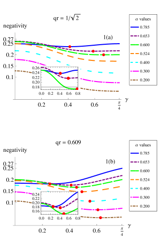
Figure 1: (Color online) Negativity of quantum state $\rho_{AB_{\mathrm{I}}}^{\Phi^{+}}$. Part (a) and (b) show the cases of $q_{R}=\frac{1}{\sqrt{2}}$ and $q_{R}=0.609$ respectively. The dot-point on the line denotes the point of variation of the curve. The small box inside the figure displays the negativity of quantum states with $\alpha=0.785$,$\alpha=0.653$ and $\alpha=0.600$ for $\rho_{AB_{\mathrm{I}}}^{\Phi_{+}}$. Some quantum states reveals clearly the entanglement amplification as acceleration increases. Here $\gamma=\frac{\pi}{4}$ denotes the infinite acceleration.

The entanglement of quantum state is measured by negativity, which evaluates the sum of negative eigenvalues of the partial transposed density matrix. The entanglement behavior at $q_{R}=\frac{1}{\sqrt{2}}$ is depicted in Fig. 1(a). In fact similar analysis was reported in ref:montero2 and ref:montero4 . The entanglement of the quantum state is decreased to the dot-point on the line. However after that point the entanglement of the state begins to increase, as Bob moves in more accelerated frame. It means the entanglement amplification of the quantum state in terms of acceleration. It is very surprising phenomena, since it is commonly believed that the entanglement may not be generated by acceleration. Fig.1 shows that the entanglement of some quantum states in fermionic system violates the common belief. As seen in Fig. 1, lesser entangled the initial state is,to more right position the point of variation moves. For the state $\Phi^{+}(\alpha)$ the increase of entanglement happens up to $\alpha=0.523599$ when $q_{R}=\frac{1}{\sqrt{2}}$. That is, the amplification of entanglement can be clearly seen between $\frac{\pi}{4}\geq\alpha\geq 0.523599$, when $q_{R}=\frac{1}{\sqrt{2}}$. The entanglement amplification at $q_{R}=0.609$ can be found in Fig. 1(b). In this case some quantum states in the accelerated frame reveals more entanglement than that in an inertial one.

We next consider the entanglement between Alice and Bob, when they share the following state,

$$|\Phi^{-}(\alpha)\rangle=\cos\alpha|0\rangle_{M}|0\rangle_{U}+\sin\alpha|1\rangle_{M}|1^{-}\rangle_{U}.$$ (4)

As it is explained previously, Bob has inaccessible part due to his acceleration. The state of Alice and Bob after tracing the region $II$ can be found. Actually as far as entanglement is concerned, the entanglement behavior of $\Phi^{+}(\alpha)$ seems to be equivalent to that of $\Phi^{-}(\alpha)$, which was discussed in ref:montero5 .
We now consider pure entangled states such as Eq. (5), when Bob is traveling with a uniform acceleration, as follows:

$$|\Phi^{*}(\alpha)\rangle=\cos\alpha|0\rangle_{M}|1^{+}\rangle_{U}+\sin\alpha|1\rangle_{M}|0\rangle_{U}.$$ (5)

As it is done before, the state that Alice and Bob share can be obtained beyond the single-mode approximation. The state when Bob is in region $I$ is obtained by tracing the other region,

$$\rho_{AB_{\mathrm{I}}}^{\Phi^{*}} = q_{L}^{2}\cos^{2}\alpha\cos^{2}\gamma|000\rangle\langle 000|$$

$$+ \frac{1}{2}(1-(1-2q_{L}^{2})\cos 2\gamma)\cos^{2}\alpha|010\rangle\langle 010|$$

$$+ \frac{q_{R}}{2}\cos^{3}\gamma\sin 2\alpha|010\rangle\langle 100|+|100\rangle\langle 010|)$$

$$+ \cos^{4}\gamma\sin^{2}\alpha|100\rangle\langle 100|$$

$$- \frac{q_{R}q_{L}}{2}\sin^{2}\alpha\sin 2\gamma(|000\rangle\langle 011|+|011\rangle\langle 000|)$$

$$- \frac{q_{L}}{2}\sin 2\alpha\cos^{2}\gamma\sin\gamma(|000\rangle\langle 101|+|101\rangle\langle 000|)$$

$$+ q_{R}^{2}\cos^{2}\alpha\sin^{2}\gamma|011\rangle\langle 011|$$

$$+ \frac{q_{R}}{2}\sin 2\alpha\cos\gamma\sin^{2}\gamma(|011\rangle\langle 101|+|101\rangle\langle 011|)$$

$$+ \frac{1}{4}\sin^{2}\alpha\sin^{2}2\gamma(|101\rangle\langle 101|+|110\rangle\langle 110|)$$

$$+ \frac{q_{L}}{2}\sin^{3}\gamma\sin 2\alpha(|010\rangle\langle 111|+|111\rangle\langle 010|)$$

$$+ \sin^{2}\alpha\sin^{4}\gamma|111\rangle\langle 111|.$$

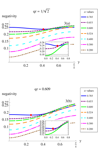
Figure 2: (Color online) Negativity of quantum state $\rho_{AB_{\mathrm{I}}}^{\Phi^{*}}$. Part (a) and (b) show the cases of $q_{R}=\frac{1}{\sqrt{2}}$ and $q_{R}=0.609$ respectively. The dot-point on the line denotes the point of variation of the curve. The small box inside the figure displays the negativity of quantum states with $\alpha=0.785$,$\alpha=0.653$ and $\alpha=0.600$ for $\rho_{AB_{\mathrm{I}}}^{\Phi^{*}}$. Some quantum states reveal clearly the entanglement amplification as acceleration increases. Here $\gamma=\frac{\pi}{4}$ denotes the infinite acceleration.

The entanglement behavior for the quantum state $\Phi^{*}(\alpha)$ at $q_{R}=\frac{1}{\sqrt{2}}$ can be seen in Fig. 2(a). We observe the point of variation as well as the amplification of entanglement, for certain quantum states. However, its entanglement behaves differently from that of state $\Phi^{+}(\alpha)$. The main difference is that the entanglement for some range of $\alpha$ does not decrease rather increases as Bob’s acceleration is getting larger. For example, the quantum state with $\alpha=0.653$ at $q_{R}=\frac{1}{\sqrt{2}}$, can get the maximal entanglement at the infinite acceleration. That is, the entanglement of the quantum state with specific $q_{R}$ and $\alpha$ has the largest value at the infinite acceleration. It seems to be a strange property, since the acceleration is believed to reduce the entanglement of the quantum state. At $q_{R}=0.609$, the behavior of entanglement can be found in Fig. 2(b).

III.b 2 party mixed entangled state

Up to now, we have considered entanglement of pure states in fermionic system when one of parties is traveling with a uniform acceleration. We have observed that there is an amplification of entanglement when a partner sharing a pure quantum state moves in accelerated frame. In this subsection, we consider a more complicate scenario when two parties share a mixed state. It is aimed to find how the entanglement behavior depends on the mixedness property, and also if its amplification is related to the mixedness. In particular, the case when a white noise is added to a maximally entangled states, so-called Werner state, is to be considered. The mixedness of Werner states is parameterized by a single parameter. So we suppose that two parties Alice and Bob prepare Werner states in inertial frames, and then Bob moves in the uniformly accelerated frame. That is, the initial state of Alice and Bob can be expressed as follows,

$$\rho_{W}=F|\Phi_{+}(\alpha=\pi/4)\rangle\langle\Phi_{+}(\alpha=\pi/4)|+\frac{1-F}{4}\mathbb{I},$$ (6)

where the maximally entangled state is taken from Eq. (3) when $\alpha=\pi/4$.

Suppose that Bob moves in an accelerated frame. Beyond the single-mode approximation, the state that Alice and Bob share in Bob’s region $I$ is obtained by tracing the region $II$, as follows,

$$\rho_{AB_{\mathrm{I}}}^{W} = \frac{1}{2}Fq_{R}\cos^{3}\gamma(|000\rangle\langle 110|+|110\rangle\langle 000|)+\frac{1}{8}\cos^{2}\gamma(3-2q_{R}^{2}+F(1-2q_{R}^{2})+(1-F)\cos 2\gamma)|100\rangle\langle 100|$$

$$+ \frac{1}{8}\cos^{2}\gamma(3-2q_{R}^{2}-F(1-2q_{R}^{2})+(1+F)\cos 2\gamma)|000\rangle\langle 000|-\frac{Fq_{L}}{2}\cos^{2}\gamma\sin\gamma(|001\rangle\langle 100|+|100\rangle\langle 001|)$$

$$+ \frac{Fq_{R}}{2}\cos\gamma\sin^{2}\gamma(|001\rangle\langle 111|+|111\rangle\langle 001|)+\frac{Fq_{L}}{2}\sin^{3}\gamma(|011\rangle\langle 110|+|110\rangle\langle 011|)$$

$$+ \frac{1}{4}\sin^{2}\gamma((1+F)q_{R}^{2}+(1-F)\sin^{2}\gamma)|111\rangle\langle 111|+\frac{1}{4}\sin^{2}\gamma((1-F)q_{R}^{2}+(1+F)\sin^{2}\gamma)|011\rangle\langle 011|$$

$$- \frac{1}{8}(1-F)q_{L}q_{R}\sin 2\gamma(|000\rangle\langle 011|+|011\rangle\langle 000|)-\frac{1}{8}(1+F)q_{L}q_{R}\sin 2\gamma(|100\rangle\langle 111|+|111\rangle\langle 100|)$$

$$+ \frac{1}{16}(1-F)\sin^{2}2\gamma|101\rangle\langle 101|+\frac{1}{16}(1+F)\sin^{2}2\gamma|001\rangle\langle 001|+\frac{1}{16}(2(1+F)-2(1+F)(1-2q_{R}^{2})\cos 2\gamma$$

$$+(1-F)\sin^{2}2\gamma)|110\rangle\langle 110|+\frac{1}{16}(2(1-F)-2(1-F)(1-2q_{R}^{2})\cos 2\gamma+(1+F)\sin^{2}2\gamma)|010\rangle\langle 010|$$

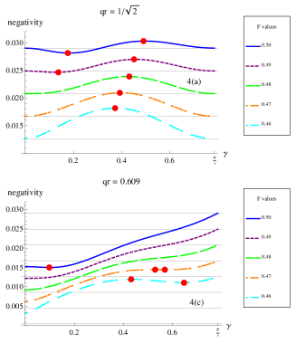
Figure 3: (Color online) Negativity of quantum state $\rho_{AB_{\mathrm{I}}}^{W}$. Part (a) and (b) show the cases of $q_{R}=\frac{1}{\sqrt{2}}$ and $q_{R}=0.609$ respectively. The dot-point on the line denotes the point of variation of the curve. Some quantum states display two dot-points, implying that there are two regions for entanglement behavior. Part (a) and (b) show clearly the entanglement amplification as acceleration increases. Here $\gamma=\frac{\pi}{4}$ denotes the infinite acceleration.

The negativity in Fig.3 depicts the entanglement amplification for some Werner states. It implies that when the mixed states are considered, their entanglement for certain mixed states shows the amplification behavior. Specially the point of variation can be found two times for the Werner state with $F=0.50$ at $q_{R}=\frac{1}{\sqrt{2}}$. In fact it happens in the Wener state of $F=0.50$ at $q_{R}=\frac{1}{\sqrt{2}}$ or $F=0.49$ at $q_{R}=\frac{1}{\sqrt{2}}$ or $F=0.47$ at $q_{R}=0.609$ or $F=0.46$ at $q_{R}=0.609$. It means that there are two regions of entanglement amplification for the states, which seems to be a peculiar property of mixed states.
We now consider the mixed entangled states such as Eq. (7), when Bob is traveling with a uniform acceleration, as follows:

$$\rho_{WL} = F|\Phi_{+}(\alpha=\pi/4)\rangle\langle\Phi_{+}(\alpha=\pi/4)|$$ (7)

$$+ \frac{1-F}{2}(|01\rangle\langle 01|+|10\rangle\langle 10|),$$

where the maximally entangled state is taken from Eq. (3) when $\alpha=\pi/4$. As it is done before, the state that Alice and Bob share can be obtained beyond the single-mode approximation. The state when Bob is in region $I$ is obtained by tracing the other region,

$$\rho_{AB_{\mathrm{I}}}^{WL}=\frac{1}{2}Fq_{R}\cos^{3}\gamma(|000\rangle\langle 110|+|110\rangle\langle 000|)$$

$$+ \frac{1}{2}\cos\gamma^{2}(F(q_{L}^{2})+(1-F)\cos\gamma^{2})|100\rangle\langle 100|$$

$$+ \frac{1}{2}\cos\gamma^{2}((1-F)(q_{L}^{2})+F\cos\gamma^{2})|000\rangle\langle 000|$$

$$+ \frac{1}{16}(1+3F-4F(1-2q_{R}^{2})\cos 2\gamma-(1-F)\cos 4\gamma)|110\rangle\langle 110|$$

$$- \frac{1}{2}Fq_{L}\cos\gamma^{2}\sin\gamma(|001\rangle\langle 100|+|100\rangle\langle 001|)$$

$$+ \frac{1}{2}Fq_{R}\cos\gamma\sin\gamma^{2}(|001\rangle\langle 111|+|111\rangle\langle 001|)$$

$$+ \frac{1}{2}Fq_{L}\sin\gamma^{3}(|011\rangle\langle 110|+|110\rangle\langle 011|)$$

$$+ \frac{1}{2}\sin\gamma^{2}((1-F)q_{R}^{2}+F\sin\gamma^{2})|011\rangle\langle 011|$$

$$+ \frac{1}{2}(Fq_{R}^{2}\sin\gamma^{2}+(1-F)\sin\gamma^{4})|111\rangle\langle 111|$$

$$- \frac{1}{4}(1-F)q_{R}q_{L}\sin 2\gamma(|000\rangle\langle 011|+|011\rangle\langle 000|)$$

$$- \frac{1}{4}Fq_{R}q_{L}\sin 2\gamma(|100\rangle\langle 111|+|111\rangle\langle 100|)$$

$$+ \frac{1}{8}(1-F)\sin 2\gamma^{2}|101\rangle\langle 101|$$

$$+ \frac{1}{8}F\sin 2\gamma^{2}|001\rangle\langle 001|$$

$$+ \frac{1}{8}(2(1-F)(1-(1-2q_{R}^{2})\cos 2\gamma)+F\sin 2\gamma^{2})|010\rangle\langle 010|$$

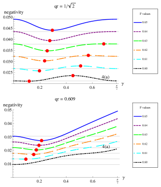
Figure 4: (Color online) Negativity of quantum state $\rho_{AB_{\mathrm{I}}}^{WL}$. Part (a) and (b) show the cases of $q_{R}=\frac{1}{\sqrt{2}}$ and $q_{R}=0.609$ respectively. The dot-point on the line denotes the point of variation of the curve. Some quantum states show clearly the entanglement amplification as acceleration increases. Here $\gamma=\frac{\pi}{4}$ denotes the infinite acceleration.

The negativity in Fig.4 shows the entanglement amplification for some mixed quantum states of Eq. (7). It implies that when the mixed states are considered, their entanglement for certain mixed states shows the amplification behavior. Specially the point of variation can be found two times for $\rho_{WL}$ with $F=0.63$ at $q_{R}=\frac{1}{\sqrt{2}}$. In fact it happens in $\rho_{WL}$ of $F=0.63$ at $q_{R}=\frac{1}{\sqrt{2}}$ or $F=0.62$ at $q_{R}=\frac{1}{\sqrt{2}}$ or $F=0.61$ at $q_{R}=\frac{1}{\sqrt{2}}$ or $F=0.60$ at $q_{R}=\frac{1}{\sqrt{2}}$.

IV. Discussion and Conclusion

We have investigated the amplification of entanglement of quantum states in fermionic system when a party sharing entangled quantum state travels in uniformly accelerated frame. Even though it has been widely believed that the acceleration may spoil the entanglement of the system, we showed that there can be the amplification of entanglement for some quantum states regardless of pure or mixed one. Also it is a surprise that some mixed states reveal two points of variation in the line of negativity. It seems to be worthwhile to investigate why there are more than one region of amplification of entanglement for some mixed states.

References

• (1) P.M. Alsing and G.J. Milburn, Phys.Rev.Lett. $\mathbf{91}$, 180404 (2003).
• (2) J.L. Ball,I. Fuentes-Schuller, and F.P. Schuller, Phys.Lett.A 359, 550 (2006).
• (3) I. Fuentes-Schuller and R.B.Mann, Phys.Rev.Lett. $\mathbf{95}$, 120404 (2005); Q.Pan and J.Jing, Phys.Rev.D $\mathbf{78}$, 065015 (2008); E. Mart$\acute{i}$n-Mart$\acute{i}$nes and J. Le$\acute{o}$n, Phys.Rev.A $\mathbf{80}$ 042318 (2010); E. Mart$\acute{i}$n-Mart$\acute{i}$nes and J. Le$\acute{o}$n, Phys.Rev.A $\mathbf{81}$ 032320 (2010).
• (4) P.M. Alsing,I. Fuentes-Schuller, R.B.Mann and T.E.Tessier, Phys.Rev.A $\mathbf{74}$, 032326 (2006).
• (5) M. Montero and E. Martín-Martínez,JEHP 07 (2011) 006.
• (6) M. Montero and E. Martín-Martínez, Phys. Rev. A $\mathbf{83}$ 062323 (2011).
• (7) M. Montero and E. Martín-Martínez, Phys. Rev. A $\mathbf{85}$, 024301 (2012).
• (8) M. Montero and E. Martín-Martínez, talk by Miguel Montero at the International Workshop in Relativistic Quantum Information North, Madrid, September 6th-8th 2011.
• (9) M. Montero and E. Martín-Martínez, Phys. Rev. A $\mathbf{84}$,012337(2011).
• (10) J.Chang and Y.Kwon, Phys.Rev. A $\mathbf{85}$, 032302 (2012).