A unifying picture of helical and azimuthal MRI, and the universal significance of the Liu limit

Abstract

The magnetorotational instability (MRI) plays a key role for cosmic structure formation by triggering turbulence in the rotating flows of accretion disks that would be otherwise hydrodynamically stable. In the limit of small magnetic Prandtl number, the helical and the azimuthal version of MRI are known to be governed by a quite different scaling behaviour than the standard MRI with a vertical applied magnetic field. Using the short-wavelength approximation for an incompressible, resistive, and viscous rotating fluid we present a unified description of helical and azimuthal MRI, and we identify the universal character of the Liu limit $2(1-\sqrt{2})\sim-0.8284$ for the critical Rossby number. From this universal behaviour we are also lead to the prediction of higher azimuthal wavenumber for rather small ratios of azimuthal to axial applied fields.

1 Introduction

The magnetorotational instability (MRI) is widely accepted as the main source of turbulence and outward angular momentum transport that is needed for the matter in accretion disks to spiral inwards onto the central proto-star or black hole, Balbus & Hawley (1991). While the early work on MRI was mainly concerned with ideal magnetohydrodynamics, the last years have seen an increasing interest in the influence of viscosity and electrical resistivity on the MRI, Pessah & Chan (2008). A particular role is thought to be played by the magnetic Prandtl number (${\rm Pm}$) which measures the ratio of viscosity to resistivity. For accretion disks around black holes (BH), Balbus & Henri (2008) had discussed the transition from large values of ${\rm Pm}$, in the vicinity of the BH, to small values in the outer part of the disk, with ${\rm Pm}$ reaching unity for approximately 100 Schwarzschild radii (depending on several parameters, among them the mass of the BH). By invoking a thermal runaway process at the unstable interface between regions with ${\rm Pm}>1$ and ${\rm Pm}<1$, the authors associated this boundary with the existence of high and low X-ray states, see Remillard & McClintock (2006).

In recent years, a vivid discussion (Lesur & Longaretti (2007); Fromang et al. (2007); Käpylä & Korpi (2011); Oishi & Mac Low (2011)) was devoted to the possible decline of the angular momentum transport rate with decreasing ${\rm Pm}$, and to the intricate roles that are played here by the magnetic Reynolds number, the detailed boundary conditions, and the stratification of the disk.

Besides this relevance to the outer part of accretion disks, to protoplanetary disks (Turner & Sano (2008)), and possibly even to planetary cores (Petitdemange et al. (2008)), the limit of low ${\rm Pm}$ has acquired some additional interest in connection with the recent liquid metal experiments devoted to the study of MRI (Sisan et al. (2004); Stefani et al. (2006); Nornberg et al. (2010)). While for the standard version of MRI (SMRI), characterized by only a vertical field being applied, the low ${\rm Pm}$ limit is rather smooth and unspectacular (Pessah & Chan (2008)), the addition of an azimuthal field leads to dramatic effects as revealed for the first time by Hollerbach & Rüdiger (2005). The arising helical MRI (HMRI), as we call it now, was shown to work also in the inductionless limit since it is governed by the Reynolds and Hartmann number, quite in contrast to SMRI which is governed by the magnetic Reynolds number and the Lundquist number. However, as it was early shown by Liu et al. (2006), the functioning of HMRI is limited to comparably steep rotation profiles with Rossby numbers ${\rm Ro}<{\rm Ro}_{Liu}=2(1-\sqrt{2})\sim-0.8284$ (which we henceforth will call the “Liu limit”), and does therefore not extend to the astrophysically important Kepler profiles characterized by ${\rm Ro}=-0.75$. This essential limitation of the HMRI, together with a variety of further parameter dependencies, was confirmed in the PROMISE experiment by Stefani et al. (2006, 2007, 2009). The intricate, though continuous, transition between SMRI and HMRI which involves a spectral exceptional point at which the inertial wave branch coalesces with the branch of the slow magnetocoriolis wave, was clarified only recently by Kirillov & Stefani (2010, 2011).

Another surprise in the limit of low $\rm Pm$ was, for the case of a purely or strongly dominant azimuthal magnetic field, the numerical prediction of a non-axisymmetric version of MRI, working apparently in a similar parameter region as HMRI (Hollerbach et al. (2010)). Although the occurrence of MRI case under the influence of a purely azimuthal magnetic field had been studied much earlier, see Hawley, Gammie and Balbus (1995); Ogilvie & Pringle (1996); Terquem & Papaloizou (1997), the crucial effect arose again for the particular combination of low $\rm Pm$ and slightly steeper than Keplerian shear profiles. It has to be noticed that this azimuthal MRI (AMRI), as we call it now, works for azimuthal magnetic fields that are current-free in the considered fluid, quite in contrast to the Tayler instability (Tayler (1973); Seilmayer et al. (2012)) that is a pinch-type instability in a current-carrying conducting medium.

The aim of this paper is to better understand why the scaling behaviour of HMRI and AMRI, and their restriction to rather steep rotation profiles, is so similar. In order to clarify this point we restrict our work completely to the short wavelength approximation (Friedlander & Lipton-Lifschitz (2003); Hattori & Fukumoto (2003)), keeping in mind that some of our conclusions will need further confirmation in more realistic simulations.

2 Short wavelength analysis of viscous, resistive MRI for arbitrary azimuthal wavenumbers

We start from the equations of incompressible, viscous and resistive magnetohydrodynamics, comprising the Navier-Stokes equation for the velocity field $\bf u$ and the induction equation for the magnetic field $\bf B$,

$$\frac{\partial{\bf u}}{\partial t}+{\bf u}\cdot\nabla{\bf u} = \frac{{\bf B}\cdot\nabla{\bf B}}{\mu_{0}\rho}-\frac{\nabla P}{\rho}+\nu\nabla^{2}{\bf u}$$ (1)

$$\frac{\partial{\bf B}}{\partial t} = {\bf B}\cdot\nabla{\bf u}-{\bf u}\cdot\nabla{\bf B}+\eta\nabla^{2}{\bf B},$$ (2)

where $P=p+\frac{{\bf B}^{2}}{2\mu_{0}}$ is the total pressure, $\rho=const$ the density, $\nu=const$ the kinematic viscosity, $\eta=(\mu_{0}\sigma)^{-1}$ the magnetic diffusivity, $\sigma$ the conductivity of the fluid, and $\mu_{0}$ the magnetic permeability of free space. Additionally, the mass continuity equation for incompressible flows and the divergence-free condition for the magnetic induction are used:

$$\nabla\cdot{\bf u}=0,\quad\nabla\cdot{\bf B}=0.$$ (3)

In the following we consider a rotational flow in the gap between the radii $R_{1}$ and $R_{2}>R_{1}$, with an imposed magnetic field sustained by currents external to the fluid (hence we disregard any version of the Tayler instability and its combination with MRI). Introducing the cylindrical coordinates $(R,\phi,z)$ we consider the stability of a magnetized Taylor-Couette (TC) flow, i.e. a steady-state background flow with the angular velocity profile $\Omega(R)$ in a (generally helical) background magnetic field,

$${\bf u}_{0}(R)=R\,\Omega(R)\,{\bf e}_{\phi},\quad p=p_{0}(R),\quad{\bf B}_{0}(R)=B_{\phi}^{0}(R){\bf e}_{\phi}+B_{z}^{0}{\bf e}_{z},$$ (4)

with the azimuthal field component

$$B_{\phi}^{0}(R)=\frac{\mu_{0}I}{2\pi R},$$ (5)

supposed to be produced by an axial current $I$.

The angular velocity profile of the background TC flow is known to have the form

$$\Omega(R)=a+\frac{b}{R^{2}},$$ (6)

where $a$ and $b$ are defined as

$$a=\frac{\mu_{\Omega}-\hat{\eta}^{2}}{1-\hat{\eta}^{2}}\Omega_{1},\quad b=\frac{1-\mu_{\Omega}}{1-\hat{\eta}^{2}}R_{1}^{2}\Omega_{1}$$ (7)

with the definitions

$$\hat{\eta}=\frac{R_{1}}{R_{2}},\quad\mu_{\Omega}=\frac{\Omega_{2}}{\Omega_{1}}.$$ (8)

Introducing, as a measure of the steepness of the rotation profile, the Rossby number $({\rm Ro})$,

$${\rm Ro}=\frac{R}{2\Omega}\frac{\partial\Omega}{\partial R}$$ (9)

we find

$$a=\Omega(1+{\rm Ro}),\quad b=-\Omega R^{2}{\rm Ro}.$$ (10)

To study flow and magnetic field perturbations on the background of the magnetized TC flow we linearize the Navier-Stokes and induction equation in the vicinity of the stationary solution by assuming ${\bf u}={\bf u}_{0}+{\bf u}^{\prime}$, $p=p_{0}+p^{\prime}$, and ${\bf B}={\bf B}_{0}+{\bf B}^{\prime}$ and leaving only terms of first order with respect to the primed quantities.

Then, by using a short-wavelength approximation (the details of the derivation will be published elsewhere) in the frame of the geometrical optics approach (see e.g. Landman & Saffman (1987); Dobrokhotov & Shafarevich (1992); Friedlander & Lipton-Lifschitz (2003); Hattori & Fukumoto (2003); Lebowitz & Zweibel (2004); Mizerski & Bajer (2009)) we end up with a system of 4 coupled equations for the perturbations of arbitrary azimuthal dependency which generalize the corresponding equations derived in Kirillov & Stefani (2010). From those 4 coupled equations, we can deduce the dispersion relation

$$p(\gamma):=\det(H-\gamma E)=0$$ (11)

generated by the matrix

$$H=\left(\begin{array}[]{cccc}-im\Omega-\omega_{\nu}&2\alpha^{2}\Omega&i\frac{m\omega_{A_{\phi}}+{\omega_{A}}}{\sqrt{\rho\mu_{0}}}&-\frac{2\omega_{A_{\phi}}\alpha^{2}}{\sqrt{\rho\mu_{0}}}\\ -2\Omega(1+{\rm Ro})&-im\Omega-\omega_{\nu}&0&i\frac{m\omega_{A_{\phi}}+{\omega_{A}}}{\sqrt{\rho\mu_{0}}}\\ i(m\omega_{A_{\phi}}+{\omega_{A}})\sqrt{\rho\mu_{0}}&0&-im\Omega-\omega_{\eta}&0\\ 2{\omega_{A_{\phi}}}{\sqrt{\rho\mu_{0}}}&i(m\omega_{A_{\phi}}+{\omega_{A}})\sqrt{\rho\mu_{0}}&2\Omega{\rm Ro}&-im\Omega-\omega_{\eta}\\ \end{array}\right)$$ (16)

where we have used the following definitions for the viscous, resistive, and the two Alfvén frequencies corresponding to the vertical and the azimuthal magnetic field:

$$\omega_{\nu} = \nu|{\bf k}|^{2}$$ (17)

$$\omega_{\eta} = \eta|{\bf k}|^{2}$$ (18)

$$\omega_{A}^{2} = \frac{k_{z}^{2}{B_{z}^{0}}^{2}}{\rho\mu_{0}}$$ (19)

$$\omega_{A_{\phi}}^{2} = \frac{(B_{\phi}^{0})^{2}}{\rho\mu_{0}R^{2}}.$$ (20)

Note that $|{\bf k}|^{2}=k^{2}_{R}+k^{2}_{z}$, and $\alpha=k_{z}/|{\bf k}|$, where $k_{R}$, $m$, and $k_{z}$ are the radial, azimuthal, and axial wavenumbers of the perturbation. In the absence of the magnetic field, the dispersion relation determined by the matrix $H$ reduces to that derived already by Krueger et al. (1966) for the non-axisymmetric perturbations of the hydrodynamical Couette-Taylor flow. Choosing, additionally, $m=0$, we reproduce the result of Eckhardt & Yao (1995). In the presence of the magnetic fields and $m=0$, we arrive at the dispersion relation derived by Kirillov & Stefani (2010).

The dispersion relation (11) generated by the matrix (16) can be rewritten completely in terms of dimensionless numbers, i.e. Rossby number $({\rm Ro})$, magnetic Prandtl number $({\rm Pm})$, ratio of the two Alfvén frequencies $(\beta)$, Hartmann number $({\rm Ha})$, Reynolds number $({\rm Re})$ and a re-scaled azimuthal wavenumber $n$:

$${\rm Pm} = \frac{\nu}{\eta}=\frac{\omega_{\nu}}{\omega_{\eta}}$$ (21)

$$\beta = \alpha\frac{\omega_{A_{\phi}}}{\omega_{A}}$$ (22)

$${\rm Re} = \alpha\frac{\Omega}{\omega_{\nu}}$$ (23)

$${{\rm Ha}} = \alpha\frac{B_{z}^{0}}{k\sqrt{\mu_{0}\rho\nu\eta}}$$ (24)

$$n = \frac{m}{\alpha}.$$ (25)

After re-scaling the spectral parameter as $\gamma=\lambda\sqrt{\omega_{\nu}\omega_{\eta}}$ we end up with the complex polynomial dispersion relation

$$p(\lambda)=a_{0}\lambda^{4}+(a_{1}+ib_{1})\lambda^{3}+(a_{2}+ib_{2})\lambda^{2}+(a_{3}+ib_{3})\lambda+a_{4}+ib_{4}=0$$ (26)

with the coefficients:

$$a_{0} = 1$$

$$a_{1} = 2\left(\sqrt{\rm Pm}+\frac{1}{\sqrt{\rm Pm}}\right)$$

$$b_{1} = 4n{\rm Re}\sqrt{\rm Pm},$$

$$a_{2} = 2(\beta^{2}{\rm Ha}^{2}-3{\rm Re}^{2}{\rm Pm})n^{2}+4\beta{\rm Ha}^{2}n+2(1+(1+2\beta^{2}){\rm Ha}^{2})+4{\rm Re}^{2}(1+{\rm Ro}){\rm Pm}+\frac{a_{1}^{2}}{4}$$

$$b_{2} = 6n{\rm Re}(1+{\rm Pm})$$

$$a_{3} = a_{1}(\beta^{2}{\rm Ha}^{2}-3{\rm Re}^{2}{\rm Pm})n^{2}+2a_{1}\beta{\rm Ha}^{2}n+a_{1}(1+(1+2\beta^{2}){\rm Ha}^{2})+8{\rm Re}^{2}(1+{\rm Ro})\sqrt{\rm Pm}$$

$$b_{3} = 4n^{3}\sqrt{\rm Pm}{\rm Re}(\beta^{2}{\rm Ha}^{2}-{\rm Re}^{2}{\rm Pm})$$

$$+ 2n{\rm Re}(4{\rm Pm}^{2}{\rm Re}^{2}(1+{\rm Ro})+(1+{\rm Pm})^{2}+2{\rm Pm}(1+{\rm Ha}^{2}))/\sqrt{\rm Pm}$$

$$- 8(1-n^{2})\beta{\rm Ha}^{2}{\rm Re}\sqrt{\rm Pm}$$

$$a_{4} = ((\beta^{2}{\rm Ha}^{2}-{\rm Re}^{2}{\rm Pm})n^{2}+2{\rm Ha}^{2}\beta n+{\rm Ha}^{2}+2{\rm Pm}{\rm Re}^{2})^{2}$$

$$+ 2(2{\rm Re}^{2}{\rm Pm}{\rm Ro}+1)(({\rm Ha}^{2}\beta^{2}-{\rm Re}^{2}{\rm Pm})n^{2}+2{\rm Ha}^{2}\beta n+{\rm Ha}^{2})-(1+{\rm Pm})^{2}{\rm Re}^{2}n^{2}$$

$$+ 4{\rm Re}^{2}(1+{\rm Ro})-({\rm Ha}^{2}+2{\rm Pm}{\rm Re}^{2})^{2}+{\rm Ha}^{4}+1+4\beta^{2}{\rm Ha}^{2}$$

$$b_{4} = 2{\rm Re}(1+{\rm Pm})(\beta^{2}{\rm Ha}^{2}-{\rm Re}^{2}{\rm Pm})n^{3}+4{\rm Re}{\rm Ha}^{2}\beta(1+{\rm Pm})n^{2}$$ (27)

$$+ 2{\rm Re}(2(1+{\rm Ro})(2{\rm Re}^{2}{\rm Pm}-\beta^{2}{\rm Ha}^{2}(1-{\rm Pm}))+(1+{\rm Ha}^{2})(1+{\rm Pm}))n$$

$$- 4\beta{\rm Ha}^{2}{\rm Re}(2+(1-{\rm Pm}){\rm Ro}).$$

Note again that this complex algebraic equation of 4th order is valid for perturbations of arbitrary azimuthal wavenumber in magnetized incompressible, viscous, resistive rotating fluids exposed to current free axial and azimuthal magnetic fields. When $n=0$ it reduces to the dispersion relation of HMRI derived by Kirillov & Stefani (2010).

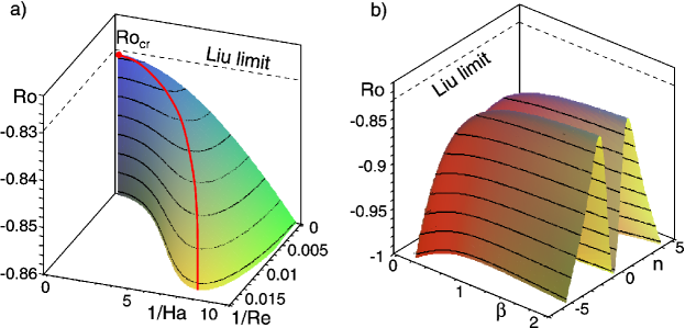
Figure 1: Inductionless limit ${\rm Pm}\rightarrow 0$: (a) At the given $n=\sqrt{2}-1/20$ and $\beta=20$ the threshold of MRI in the $({\rm Re^{-1}},{\rm Ha^{-1}},{\rm Ro})$ space with the maximum at the singular (red) point $(0,0,{\rm Ro}_{cr}=2-2\sqrt{2})$. The red line leading to the maximum projects into a curve approximated in the vicinity of the origin by the scaling law (29). (b) The threshold of MRI in the $(\beta,n,{\rm Ro})$ space with ${\rm Ha}=6$ and $\rm Re$ determined by the scaling law (29) reaches its upper bound at $\beta\rightarrow\infty$ (AMRI), which is still below the Liu limit ${\rm Ro}_{Liu}=2-2\sqrt{2}$.

3 Inductionless limit

Proceeding quite similar as in Kirillov & Stefani (2010), we apply the Bilharz criterion (Bilharz (1944)) to the complex polynomial (26) and derive the maximum Rossby number, at which flows are prone to MRI, as a function of the remaining dimensionless numbers. In the following, we concentrate on the inductionless limit, i.e. we take the limit $\rm Pm\rightarrow 0$.

After verifying the facts that the inductionless threshold value of $\rm Ro$ increases monotonically with ${\rm Re}$ so that we can take the limit ${\rm Re}\rightarrow\infty$, and that in this limit the threshold value of $\rm Ro$ increases monotonically with ${\rm Ha}$, Fig. 1(a), so that we can take the limit ${\rm Ha}\rightarrow\infty$, we obtain the following explicit expression for this maximized (with respect to $\rm Ha$ and $\rm Re$) critical Rossby number at the threshold of MRI in the inductionless limit:

$${\rm Ro}_{cr}(\beta,n) = \frac{4\beta^{4}+(\beta n+1)^{4}-(2\beta^{2}+(\beta n+1)^{2})\sqrt{4\beta^{4}+(\beta n+1)^{4}}}{2\beta^{2}(\beta n+1)^{2}}.$$ (28)

The maximum value of the Rossby number, ${\rm Ro}_{cr}$, is shown as a red dot in Fig. 1(a). When $n=0$, Eq. (28) reduces to the threshold of HMRI in the inductionless limit found in Kirillov & Stefani (2011). Given $n$ and $\beta$, the critical Rossby number calculated with finite values of $\rm Re$ and $\rm Ha$, is always below the majorating value, ${\rm Ro}_{cr}(\beta,n)$, determined by Eq. (28), see Fig. 1(b). With the increase of Ha and $\rm Re$ constrained by the scaling law

$${\rm Re}=2(1+\sqrt{2})\beta^{3}{\rm Ha}^{3},$$ (29)

the threshold shown in Fig. 1(b) tends to the majorating surface ${\rm Ro}_{cr}(\beta,n)$ shown in Fig. 2(a).

The remarkably simple dependence (28) of ${\rm Ro}_{cr}$, only on the ratio $\beta$ of azimuthal to axial field and on the rescaled azimuthal wavenumber $n$, relies on the appropriate choice of the dimensionless parameters, in particular on “hiding” the wavenumber ratio $\alpha$ in them. Assume we have fixed the sign of $\beta$, the functional dependence of the maximum critical Rossby number (28) on $\beta$ and $n$ has a two-saddle line structure as shown in Fig. 2(a).

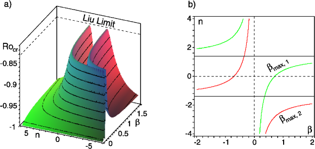
Figure 2: (a) The critical Rossby number maximized with respect to $\rm Ha$ and $\rm Re$, given by Eq. (28), in dependence on $\beta$ and $n$. (b) The lines (green) $\beta_{max,1}$ and (red) $\beta_{max,2}$ at which the function ${\rm Ro}_{cr}(\beta,n)$ attains its maximal value ${\rm Ro}_{Liu}=2-2\sqrt{2}$.

Now, the most important result of this paper is that both saddle lines have the same height everywhere, namely the Liu limit ${\rm Ro}_{Liu}=2(1-\sqrt{2})$, independent on the particular combination of $\beta$ and $n$. From Eq. (28) it can be proved that these saddle lines, with ${\rm Ro}_{Liu}=2-2\sqrt{2}$, are governed by the two equations

$$\beta_{max,1}(n) = \frac{1}{\sqrt{2}-n},\quad{\rm Ro}_{cr}(\beta_{max,1})=2-2\sqrt{2}$$

$$\beta_{max,2}(n) = \frac{-1}{\sqrt{2}+n},\quad{\rm Ro}_{cr}(\beta_{max,2})=2-2\sqrt{2}.$$ (30)

In Fig. 2(b) the curves $\beta_{max,1}(n)$ and $\beta_{max,2}(n)$ are shown in green and red colors, respectively. Note that according to the first of Eqs. (3), $n=0$ (HMRI) corresponds to $\beta=1/\sqrt{2}$ which being substituted into Eq. (29), yields the following scaling law for the optimum combination of $\rm Re$ and $\rm Ha$ in HMRI (Kirillov & Stefani (2010))

$${\rm Re}=\frac{2+\sqrt{2}}{2}{\rm Ha}^{3}.$$ (31)

Therefore, even in the case of non-axisymmetric perturbations, the maximum possible value of the Rossby number prone to the magnetorotational instability caused by the helical magnetic field in the inductionless limit is still ${\rm Ro}_{Liu}=2-2\sqrt{2}$, exactly as in the case of HMRI which is an instability with respect to the axisymmetric perturbations $(n=0)$. The relations (3) between $\beta$ and $n$ that correspond to the Liu limit give a sort of the resonance conditions between the components of the wavevector of the three-dimensional perturbation and the components of the helical magnetic field.

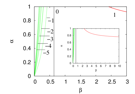
Figure 3: Range of $\alpha$ for the different $m$ modes, in dependence on $\beta$.

On the basis of the equations (3) connecting $\beta$ and the rescaled azimuthal wavenumber $n$, we can ask now for the structure of the solution in terms of the original, “physical” azimuthal wavenumber $m$. From the definition $\alpha=k_{z}/|{\bf k}|$ we see immediately that $\alpha$ can take on only values between -1 and +1. The solution structure can thus be visualized as in Fig. 3. For example, from the first of the Eqs. (3) we see that for large values of $\beta$ (AMRI), the only possible integer solution is the $m=1$ mode, whose corresponding wavenumber ratio converges than to $\alpha=1/\sqrt{2}$, see also Fig. 2(b). There is a lower limit of $\beta=1+\sqrt{2}\sim 2.41$ for this $m=1$ mode. Lowering $\beta$ further, we find next the $m=0$ mode (HMRI) to dominate at the Liu limit, restricted only to $\beta=1/\sqrt{2}$, Kirillov & Stefani (2010). Interestingly, decreasing $\beta>0$ even further to zero we find a sequence of higher azimuthal modes with the sign of $m$ that is opposite to the sign of $\beta$, which indicates a kind of resonance phenomenon.

Since $\alpha$ enters also the definition of $\beta$ it might be instructive to illustrate the mode structure also in dependence on $\beta/\alpha=\omega_{A_{\phi}}/\omega_{A}$. From Eqs. (3) we derive

$$\alpha=\pm\frac{\sqrt{2}}{2}\left(m+\frac{\omega_{A}}{\omega_{A_{\phi}}}\right),$$ (32)

where the positive sign corresponds to the first of Eqs. (3) and the negative sign to the second one. This means that with a given azimuthal wavenumber $m$, two axial wavenumbers, $k_{z}$, are associated following from Eq. (32) that differ by sign only. Such combinations of wavenumbers are the most destabilizing in the sense that the magnetized Taylor-Couette flow is unstable at the highest possible Rossby number.

In Fig. 4 we plot the positive branch of Eq. (32) because the negative one is simply its reflection about the horizontal coordinate axis. We see now the HMRI mode ($m=0$) to start at $\omega_{A_{\phi}}/\omega_{A}=1/\sqrt{2}$ and to remain for arbitrary large values of $\beta/\alpha$, although with an ever decreasing wavenumber ratio, which would correspond to ever increasing wavelengths in $z$ direction. Again it is only the AMRI modes ($m=\pm 1$) that, for large $\beta/\alpha$, maintain a physically sensible wavenumbers $\alpha=\pm 1/\sqrt{2}$. The higher modes with $m\leq-2$ are obtained for smaller values of $\beta/\alpha$.

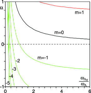
Figure 4: Range of $\alpha$ for the different $m$ modes, in dependence on $\beta/\alpha$: (red line) $m=1$, (black line) $m=0$, (green lines) $m=-1,-2,-3,-4,-5$.

Hence, when the azimuthal magnetic field is directed along the basic flow that rotates counter-clockwise with respect to $z$-axis, among the modes that are MRI-unstable at the Liu limit there are only two (AMRI) that co-rotate with the flow $(m=1)$ and simultaneously propagate either along the positive or negative $z$-direction. These modes are dominant when $\omega_{A_{\phi}}/\omega_{A}>1+\sqrt{2}$, see the red curve in Fig. 4. At moderate ratios $\omega_{A_{\phi}}/\omega_{A}$, the Liu limit is at the axisymmetric HMRI mode. When $\omega_{A_{\phi}}/\omega_{A}\rightarrow 0$, infinitely many modes with $m\leq-1$ that propagate either in the negative or positive $z$-direction and counter-rotate with respect to the basic flow can cause instability at the Liu limit. Note, however, that at finite $\rm Re$ and $\rm Ha$ the highest modes will be inhibited, see Fig. 1(b).

4 Conclusion

Using a short-wavelength approach, we have presented a unifying picture of the inductionless forms of MRI. We have identified a continuous function of the maximum critical Rossby number that incorporates both types of instability. We were lead to the conclusion that in the limit of small ratios of azimuthal to axial field there should be inductionless MRI versions with higher $m$ modes, counter-rotating with respect to the basic flow, although this needs further confirmation at least by a 1D linear stability analysis. Most interestingly, the Liu limit has turned out as being of quite universal significance, since the range of its validity has been extended from the realm of axisymmetric HMRI to that of non-axisymmetric MRI versions. Actually, soon after its derivation in the WKB approximation, the relevance of the Liu limit had been questioned by Rüdiger and Hollerbach (2007) who had found an apparent extension of this limit in global simulations when at least one of the radial boundary conditions was assumed to be electrically conducting. Later, though, utilizing another definition of the notion “quasi-Keplerian” for Taylor-Couette flows, the Liu limit was rehabilitated by Priede (2011). As a side remark, the determination of such limits is even more complicated by the necessity to distinguish, for travelling waves as in HMRI, between convective and absolute (or global) instabilities, which has been thoroughly discussed by Priede & Gerbeth (2009) and which was shown to be experimentally important by Stefani et al. (2009).

From the strictly astrophysical point of view, our support for the Liu limit may appear disappointing, since it would exclude any relevance of the inductionless versions of MRI to accretion disks with Keplerian rotation. A subtly question in this respect is, however, connected with the saturation mechanism of the MRI that could, possibly, lead to modified shear profiles. With main focus on low $\rm Pm$ flows, Umurhan (2010) had asked for the possibility that the saturation of MRI could lead to modified flow structures within parts of steeper shear, sandwiched with parts of shallower shear. By virtue of a possible sudden onset within such segments of steepening shear, the inductionless MRI versions could thus play a certain role in real astrophysical settings.

References

- Balbus & Hawley (1991) Balbus, S. A. & Hawley, J. F. 1991, ApJ, 376, 214
- Balbus & Henri (2008) Balbus, S. A. & Henri, P. 2008, ApJ, 674, 408
- Bilharz (1944) Bilharz, H. 1944, Z. angew. Math. Mech., 24, 77
- Dobrokhotov & Shafarevich (1992) Dobrokhotov, S. & Shafarevich, A. 1992, Math. Notes, 51, 47
- Eckhardt & Yao (1995) Eckhardt, B. & Yao, D. 1995, Chaos, Solitons & Fractals, 5(11), 2073
- Friedlander & Lipton-Lifschitz (2003) Friedlander, S. & Lipton-Lifschitz, A. 2003, Localized instabilities in fluids. Handbook of Mathematical Fluid Dynamics, vol. II, S.J. Friedlander and D. Serre, eds., Elsevier, 289
- Fromang et al. (2007) Fromang, S., Papaloizou, J., Lesur, G. & Heinemann, T. 2007, A&A, 476, 1123
- Hattori & Fukumoto (2003) Hattori, Y. & Fukumoto, Y. 2003, Phys. Fluids, 15, 3151
- Hawley, Gammie and Balbus (1995) Hawley, J. F., Gammie, C. F., Balbus, S. A., 1995, ApJ, 440, 742
- Hollerbach & Rüdiger (2005) Hollerbach, R. & Rüdiger, G. 2005, Phys. Rev. Lett., 95, 124501
- Hollerbach et al. (2010) Hollerbach, R., Teeluck, V. & Rüdiger, G. 2010, Phys. Rev. Lett., 104, 044502
- Käpylä & Korpi (2011) Käpylä, P. J. & Korpi, M. J. 2011, MNRAS, 413, 901
- Kirillov & Stefani (2010) Kirillov, O. N. & Stefani, F. 2010, ApJ, 712, 52
- Kirillov & Stefani (2011) Kirillov, O. N. & Stefani, F. 2011, Phys. Rev. E, 84, 036304
- Krueger et al. (1966) Krueger, E. R., Gross, A., Di Prima, R. C., J. Fluid Mech., 1966, 24(3), 521
- Landman & Saffman (1987) Landman, M. J. & Saffman P. G. 1987, Phys. Fluids, 30, 2339
- Lebowitz & Zweibel (2004) Lebovitz, N. R. & Zweibel E. 2004, ApJ, 609, 301
- Lesur & Longaretti (2007) Lesur, G. & Longaretti, P.-Y. 2007, MNRAS, 378, 1471
- Liu et al. (2006) Liu, W., Goodman, J., Herron, I. & Ji, H. T. 2006, Phys. Rev. E, 74, 056302
- Mizerski & Bajer (2009) Mizerski, K. A. & Bajer, K. 2009, J. Fluid. Mech., 632, 401
- Nornberg et al. (2010) Nornberg, M. D., Ji, H., Schartman, E., Roach, E. & Goodman, J. 2010, Phys. Rev. Lett., 104, 074501
- Ogilvie & Pringle (1996) Ogilvie, G. I. & Pringle, J. E. 1996, MNRAS, 279, 151
- Oishi & Mac Low (2011) Oishi, J. S. & Mac Low, M.-M. 2011, ApJ, 740, 18
- Pessah & Chan (2008) Pessah, M. E. & Chan, C. 2008, ApJ, 684, 498
- Petitdemange et al. (2008) Petitdemange, L., Dormy, E. & Balbus, S. A. 2008, Geophys. Res. Lett., 35, 15305
- Priede (2011) Priede, J. 2011, Phys. Rev. E, 84, 066314
- Priede & Gerbeth (2009) Priede, J. & Gerbeth, G. 2009, Phys. Rev. E 79, 046310
- Remillard & McClintock (2006) Remillard, R. A. & McClintock, J. E. 2006, Annu. Rev. Astron. Astrophys., 44, 49
- Rüdiger and Hollerbach (2007) Rüdiger, G. & Hollerbach, R. 2007, Phys. Rev. E, 76, 068301
- Seilmayer et al. (2012) Seilmayer, M., Stefani, F., Gundrum, T., Weier, T., Gerbeth, G., Gellert, M. & Rüdiger, G. 2012, Phys. Rev. Lett., in press, arXiv 1112.2103
- Sisan et al. (2004) Sisan, D. R., Mujica, N., Tillotson, W. A., Huang, Y. M., Dorland, A. B., Hassam, A. B., Antonsen, T. M. & Lathrop, D. P. 2004, Phys. Rev. Lett., 93, 114502
- Stefani et al. (2006) Stefani, F., Gundrum, T., Gerbeth, G., Rüdiger, G., Schultz, M., Szklarski, J. & Hollerbach, R. 2006, Phys. Rev. Lett., 97, 184502
- Stefani et al. (2007) Stefani, F., Gundrum, T., Gerbeth, G., Rüdiger, G., Szklarski, J. & Hollerbach, R. 2007, New J. Phys., 9, 295
- Stefani et al. (2009) Stefani, F., G. Gerbeth, Gundrum, T., Hollerbach, R., Priede, J., Rüdiger, G., & Szklarski, J., 2009, Phys. Rev. E., 80, 066303
- Tayler (1973) Tayler, R. J. 1973, MNRAS, 161, 365
- Terquem & Papaloizou (1997) Papaloizou, J. C. B. & Terquem, C. 2007, MNRAS, 287, 771
- Turner & Sano (2008) Turner, N. J. & Sano, T. 2008, ApJ, 679, L131
- Umurhan (2010) Umurhan, O. M. 2010, A&A, 513, A47