Neutrino mass determination from a four-zero texture mass matrix.

Abstract

We analyze the different parametrizations of a general four-zero texture mass matrices for quarks and leptons, that are able to reproduce the CKM and PMNS mixing matrices. This study is done through a $\chi^{2}$ analysis. In quark sector, only four solutions are found to be compatible with CKM mixing matrix. In leptonic sector, using the last experimental results about the mixing angles in the neutrino sector, our $\chi^{2}$ analysis shows a preferred value for $m_{\nu_{3}}$ to be around $0.05$ $eV$ independently of the parametrization of the four-zero texture mass matrices chosen for the charged leptons and neutrinos.

I Introduction

The Yukawa sector of the Standard Model (SM) parametrizes the main phenomenological characteristics of fermions with respect to mass and flavor. Although there is increasing information on the numerical values of these parameters, a fundamental understanding of their origin is currently lacking. The total number of families, the smallness of neutrino masses,the origin of CP violation, the mass spectrum, are among the problems that still have no answer within the SM. A phenomenological approach to these questions is to assume some general textures for the Yukawa matrices for quarks and leptons and then to compare with experimental data on flavor mixing. The interesting point in this approach is that the hidden symmetry existing in the proposed textures could give some hints on how to extend the Standard Model gauge symmetries. For each chosen textures for Yukawa matrices, it is possible to relate mixing angles and fermion masses Joglekar (1977); Wilczek and Zee (1977); Fritzsch (1977); Leurer et al. (1993); Ramond et al. (1993); Ibanez and Ross (1994) and then to compare to our experimental knowledge on fermion masses and mixing Fritzsch (1978, 1979); Fritzsch and Xing (2000); Pakvasa and Sugawara (1978); Harari et al. (1978); Fritzsch and Xing (1995, 2003); Randhawa et al. (2006); Dev et al. (2009); Gupta and Ahuja (2011). Most of the studies have been done for the quarks sector but some analysis have been made using a six-zero texture related with neutrinos Xing (2002a); Branco et al. (2009) using an hermitian mass matrix. These models have been ruled out by experimental bounds on mixing angles Du and Xing (1993); Fritzsch and Xing (2003); Frampton et al. (2002); Aaij et al. (2011). Other kind of textures have been proposed for leptonic sector as the one-zero texture Merle and Rodejohann (2006); Lashin and Chamoun (2011) and single or double vanishing minors Lashin and Chamoun (2008, 2009); Lashin et al. (2011) with relative success.

Another promising texture candidate is the four-zero texture which seems to be a good candidate to reproduce the CKM matrix mixing elements Fritzsch (1978, 1979); Fritzsch and Xing (2000, 2003). Usually, it has been assumed for the four-zero textures that fermion masses matrices are hermitian Fritzsch (1978, 1979); Fritzsch and Xing (2000); Branco et al. (2000); Zhou (2003); Fritzsch and Xing (2003); Matsuda and Nishiura (2006). It has been pointed out that all fermions sectors can be described with the same formalism, like in $SO(10)$ Great Unification models Dev et al. (2012); Buchmuller and Wyler (2001); Bando and Obara (2003) or assuming discrete symmetry groups Pakvasa and Sugawara (1978); Harari et al. (1978); Fritzsch and Xing (2000); Xing and Zhang (2003). Hence, it is natural to consider that the same texture-mass matrix could be used for both quarks and leptons Xing (2002b); Hu et al. (2011); Barranco et al. (2010); Gonzalez Canales and Mondragon (2011). Previous works have analysed the relation between the quark masses hierarchy and the CKM matrix in hermitian case for the four-zero texture Branco et al. (2000); Zhou (2003); Fritzsch and Xing (2003) and more recently some studies have included a unified four-zero texture for both the leptonic and the quark sectors Matsuda and Nishiura (2006); Barranco et al. (2010); Gonzalez Canales et al. (2011). The later analysis shown that hermitian four-zero texture are compatibles with experimental results on quark and leptonic masses as well as CKM and PMNS mixing angles.

In this work, we shall focus on a general four-zero texture parametrization for quarks and leptons Yukawa matrices without the hermiticity assumption usually done for these matrices. From these general four-zero texture parametrization, we shall extensively study all the solutions obtained for the fermion masses and mixing. We shall demonstrate that using as input parameters the fermion masses, all the solutions can be described through an extra free parameters for each Yukawa matrices. Then these free parameters will be fine-tuned in order to reproduce both the Cabibbo-Kobayashi-Maskawa (CKM) and the Pontecorvo Maki Nakagawa Sakata (PMNS) matrices. The fit is done by a $\chi^{2}$ analysis and we find that from all the parametrizations the current data on CKM mixing angles excludes all except four parametrizations. In the leptonic sector, the absolute neutrino masses are unknown. We shall show that in order to reproduce the PMNS mixing angles the neutrino mass of the heaviest neutrino should be around $\sim 0.05$ eV, a result that is independent of the parametrization used. From this, we can conclude that in order to have a good fit on the leptonic mixing angle by assuming a four zero texture mass matrix the absolute neutrino masses will be fixed. Our analysis is new compared to previous similar analysis Matsuda and Nishiura (2006) in three aspects:

• We update the latest results on leptonic mixing angle $\sin\theta_{13}$ and we show that with this value of $\sin\theta_{13}$, the assumptions to have a four-zero textures for the Yukawa matrices fix the neutrino mass scale to be around 0.05 eV.

• We study all possible parametrizations of the mixing angles in terms of the fermion masses.

• We avoid any approximations since the precision data on CKM mixing and the PMNS mixing impose a precise fine-tuning of the free parameters.

In addition, we shall show that the assumption of hermitian four-zero texture matrices is not necessary. Actually, within the SM, Yukawa couplings need not be either symmetric or hermitian, therefore it is interesting to complement these kind of analyses by looking Yukawa couplings that are not necessarily hermitian Branco and Silva-Marcos (1994). Furthermore, non-hermitian mass matrices can be obtained in some models with discrete symmetries, such as the $S_{3}$ models Mondragon et al. (2011).

This paper is divided in following sections. In Section II, we explicitly show the process to diagonalize the general four-zero texture mass matrices and obtain all possible different parametrizations in terms of the fermion masses. Then, the mixing matrices are obtained. In section III, we analyze the different solutions obtained from diagonalization through a $\chi^{2}$ analysis using the up-to-date experimental values for the CKM and PNMS mixing matrices. Finally in section IV, we present our conclusions.

II Parametrizations of four-zero texture mass matrices

We assume that the Yukawa matrices have a non-hermitian four-zero texture in the flavor basis which is given by

$$M^{f}=\left(\begin{array}[]{ccc}0&C_{f}&0\\ C^{\prime}_{f}&D_{f}&B_{f}\\ 0&B^{\prime}_{f}&A_{f}\end{array}\right).$$ (1)

In hermitian case, one has to assume that $C^{\prime}_{f}=C_{f}^{*}$ and $B^{\prime}_{f}=B_{f}^{*}$. Here we only assume that $|C_{f}|=|C^{\prime}_{f}|$ and $|B_{f}|=|B^{\prime}_{f}|$ but the phases can be different Branco and Silva-Marcos (1994); Mondragon et al. (2011).

The most general diagonalization of Yukawa matrix must be done trough a bilinear transformation. In the case of three generations:

$$U_{L}^{f\dagger}M^{f}U_{R}^{f}=\text{diag}(m_{1}^{f},m_{2}^{f},m_{3}^{f}),$$ (2)

where $f=u,d,\ell$ is a flavor index and $\{U^{f}_{L},U_{R}^{f}\}$ are $SU(3)$ matrices. By definition, the eigenvalues of $M^{f}$ must be the masses of fermions, thus they are real. For a general matrix, the unitary matrices are found solving the equations

$$U_{L}^{f\dagger}M^{f}M^{f\dagger}U_{L}^{f} = \text{diag}(m_{1}^{f2},m_{2}^{f2},m_{3}^{f2}),$$ (3)

$$U_{R}^{f\dagger}M^{f\dagger}M^{f}U_{R}^{f} = \text{diag}(m_{1}^{f2},m_{2}^{f2},m_{3}^{f2}),$$ (4)

for $U_{L}$ and $U_{R}$. From now on, we omit the index $f$ for short. The $H\equiv MM^{\dagger}$ matrix can be easily computed with the matrix (1) as

$$H=\left(\begin{array}[]{ccc}|C|^{2}&CD^{*}&CB^{\prime*}\\ DC^{*}&|B|^{2}+|C^{\prime}|^{2}+|D|^{2}&B^{\prime*}D+A^{*}B\\ B^{\prime}C^{*}&B^{\prime}D^{*}+AB^{*}&|A|^{2}+|B^{\prime}|^{2}\\ \end{array}\right).$$ (5)

This is a hermitian matrix and can be diagonalized by an unitary transformation. Writing $B(B^{\prime})=be^{i\phi_{B}(\phi_{B^{\prime}})}$, $C(C^{\prime})=ce^{i\phi_{C}(\phi_{C^{\prime}})}$, $D=de^{i\phi_{D}}$ and $A=ae^{i\phi_{A}}$ it is possible to separate the phases of the non-diagonal elements, throughout the unitary transformation

$$H=P^{\dagger}\tilde{H}P,$$ (6)

where $P=e^{-\frac{i}{2}\Xi}\text{diag}\left(e^{\frac{i}{2}\Xi},e^{i(\phi_{C}-\phi_{D})},e^{i(\phi_{C}+\phi_{B^{\prime}}+\Xi)}\right)$ and

$$\Xi=\arctan\left[\frac{a\sin(\phi_{B}+\phi_{B^{\prime}}-\phi_{A}-\phi_{D})}{d+a\cos(\phi_{B}+\phi_{B^{\prime}}-\phi_{A}-\phi_{D})}\right].$$ (7)

Then we have that $\tilde{H}$ is real and symmetric that depends on four positive parameters and one combination of phases, that is

$$\tilde{H}=\left(\begin{array}[]{ccc}c^{2}&cd&bc\\ cd&c^{2}+d^{2}+b^{2}&b|d+a\delta|\\ bc&b|d+a\delta^{*}|&a^{2}+b^{2}\\ \end{array}\right),$$ (8)

where $\delta=e^{i(\phi_{D}-\phi_{B^{\prime}}-\phi_{B}+\phi_{A})}$. The matrix (8) can be diagonalized by an orthogonal matrix $\mathcal{O}_{ij}=v_{i}(m_{j}^{2})$, formed with the $i$ component of the eigenvectors $\mathbf{v}(m_{i}^{2})$ that arises from the solution of $(\tilde{H}-m^{2}_{i}1_{3\times 3})\textbf{v}(m_{i}^{2})=\textbf{0}$, where $m_{i}^{2}$ are the eigenvalues of $\tilde{H}$. Therefore the unitary matrix that diagonalizes (5) is given by $U_{L}=\mathcal{O}P$. Because the diagonalization of $\tilde{H}$ is performed by an orthogonal transformation, the invariants under this transformations give the system

$$\text{Tr}(\tilde{H}) = m_{1}^{2}+m_{2}^{2}+m_{3}^{2},$$

$$\text{Tr}^{2}(\tilde{H})-\text{Tr}(\tilde{H^{2}}) = 2m_{1}^{2}m_{2}^{2}+2m_{1}^{2}m_{3}^{2}+2m_{2}^{2}m_{3}^{2},$$

$$\text{Det}(\tilde{H}) = m^{2}_{1}m^{2}_{2}m^{2}_{3},$$ (9)

that reduce the number of free parameters when we solve for $b$, $c$ and $d$ in terms of the eigenvalues $m_{i}^{2}$, the parameter $a$ and the phase $\delta$. Thus the components of the i-eigenvector of $\tilde{H}$ is given by

$$v_{1}(m_{i}^{2},a,\delta) = (b^{2}+c^{2}-cd+d^{2}-m_{i}^{2})(a^{2}-b|d+a\delta|+b^{2}-m_{i}^{2})$$

$$-b(c-|d+a\delta|)(-b|d+a\delta|+b^{2}+c^{2}+d^{2}-m_{i}^{2}),$$

$$v_{2}(m_{i}^{2},a,\delta) = -m_{i}^{2}(a^{2}+b^{2}+c^{2}-cd)+c(a^{2}+bd)(c-d)$$

$$+b\left[c(b-c)+m_{1}^{2}\right]|d+a\delta|+m_{i}^{4},$$

$$v_{3}(m_{i}^{2},a,\delta) = \left[c(d-c)-m_{i}^{2}\right](b^{2}+c^{2}+d^{2}-b|d+a\delta|-m_{i}^{2})$$ (10)

$$+c(b-d)(b^{2}+c^{2}-cd+d^{2}-m_{i}^{2}).$$

From a general analysis of the solutions of previous equations, the only solutions corresponding to eigenvalues given by $m_{1,2,3}^{2}$, i.e. , independent of the other free parameters, are given only when $\Xi_{f}=0$ for $f=u,d,\ell,\nu$. Using this property, the diagonal matrix of phases can be written as $P^{f}=\text{diag}(1,e^{i\phi^{f}_{1}},e^{i\phi^{f}_{2}})$, where $\phi^{f}_{1}\equiv\phi_{C_{f}}-\phi_{D_{f}}$ and $\phi^{f}_{2}\equiv\phi_{C_{f}}+\phi_{B_{f}^{\prime}}$ for $f=u,d,\ell,\nu$. As expected, the hermitian case can be reached if the phases are constrained to $\phi_{D_{f}}=0$ and $\phi_{B_{f}}=-\phi_{B^{\prime}_{f}}$. It is important to stress that the relations between the elements of the mixing matrix and the masses are not the same than in the hermitian case.

The system (II) has formally 32 solutions that are closely related by chiral transformations that basically change the sign of the masses $m_{i}$, thus without loss of generality we can assumed that $m_{i}>0$, where $i=1,2,3$, and adjust the interval of possible values that the free parameters can take. Once the restrictions on parameters and the normal order of masses $m_{1}<m_{2}<m_{3}$ are introduced, the number of independent solution is reduce to three. This means that exist three independent parametrizations for $U^{f}_{L}$ that diagonalize $H$. Such parametrizations are given by

$${\rm Parametrization\quad 1}\qquad\tilde{m}_{1}\leq a^{\prime}\leq\tilde{m}_{2}\quad\left\{\begin{array}[]{ccc}b^{\prime}&=&\sqrt{\frac{(a^{\prime}-\tilde{m}_{1})(-a^{\prime}+\tilde{m}_{2})(\tilde{m}_{3}+a^{\prime})}{a^{\prime}}}\\ d^{\prime}&=&-a^{\prime}+\tilde{m}_{1}+\tilde{m}_{2}-\tilde{m}_{3}\end{array}\right.$$ (11)

$${\rm Parametrization\quad 2}\qquad\tilde{m}_{1}\leq a^{\prime}\leq\tilde{m}_{3}\quad\left\{\begin{array}[]{ccc}b^{\prime}&=&\sqrt{\frac{(a^{\prime}-\tilde{m}_{1})(a^{\prime}+\tilde{m}_{2})(\tilde{m}_{3}-a^{\prime})}{a^{\prime}}}\\ d^{\prime}&=&-a^{\prime}+\tilde{m}_{1}-\tilde{m}_{2}+\tilde{m}_{3}\end{array}\right.$$ (12)

$${\rm Parametrization\quad 3}\qquad\tilde{m}_{2}\leq a^{\prime}\leq\tilde{m}_{3}\quad\left\{\begin{array}[]{ccc}b^{\prime}&=&\sqrt{\frac{(a^{\prime}+\tilde{m}_{1})(a^{\prime}-\tilde{m}_{2})(\tilde{m}_{3}-a^{\prime})}{a^{\prime}}}\\ d^{\prime}&=&-a^{\prime}-\tilde{m}_{1}+\tilde{m}_{2}+\tilde{m}_{3}\end{array}\right.$$ (13)

where for all cases $c^{\prime}=\sqrt{\frac{\tilde{m}_{1}\tilde{m}_{2}\tilde{m}_{3}}{a^{\prime}}}$. Here the parameters $a^{\prime}=\frac{a}{m_{3}}$, $b^{\prime}=\frac{b}{m_{3}}$, $c^{\prime}=\frac{c}{m_{3}}$ and $d^{\prime}=\frac{d}{m_{3}}$ have been defined. Likewise the scaled masses are $\tilde{m}_{i}=\frac{m_{i}}{m_{3}}$ for $i=1,2,3$; here one can see that $\tilde{m}_{3}=1$.

As seen in the parametrizations (11-13) the factor $a^{\prime}$ ranges between a minimal $\tilde{m}_{\text{min}}$ and maximal $\tilde{m}_{\text{max}}$ value due to the restriction $b^{\prime}>0$. This allows to write a linear dependence of $a^{\prime}$ in terms of $\tilde{m}_{i}$’s and a free parameter $x_{f}$:

$$a^{\prime}_{1}(x_{f})=\tilde{m}_{max}\left(1-x_{f}\frac{\tilde{m}_{max}-\tilde{m}_{min}}{\tilde{m}_{max}}\right).$$ (14)

With this we have a complete description for parameters of $M^{f}$ in terms of $\tilde{m}_{i}^{f}$ and $x_{f}$ for $\delta=1$. The fact that we have three parametrizations for each fermion mass matrix (up and down) say that there are 9 possibilities to construct the $V_{\rm CKM}$ and $U_{\rm MNS}$ matrices.

III Fitting $V_{\rm CKM}$ and $U_{\rm MNS}$

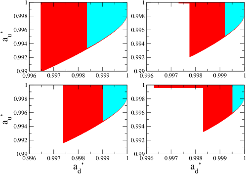
Figure 1: Allowed values of parameters $a^{\prime}_{u},a^{\prime}_{d}$ that fit CKM matrix elements. Red is 90% C.L. and cyan is 68% C.L. Top-left panel corresponds to picking-up the parametrization 2 (eq. 12) for both the u-type and d-type quarks. Top-right panel corresponds to parametrization 2 for the u-type quarks and parametrization 3 (eq. 13) for the d-type quarks. Bottom-left panel corresponds to parametrization 3 for the u-type quarks and parametrization 2 for d-type quarks. Finally, bottom-right panel shows the allowed region when parametrization 3 is used for both u and d type quarks.

Let us summarize the previous section. The real and symmetric matrix $\tilde{H}$ is diagonalized with the help of the eigenvectors (II). The elements $a^{\prime},b^{\prime},c^{\prime},d^{\prime}$ are real and can be inverted with the help of the invariants (II) into functions of the masses $\tilde{m}_{j}$ and since we have only three invariants, we can choose $a^{\prime}$ as a free parameter. Then, $b^{\prime}=b^{\prime}(\tilde{m}_{j},a^{\prime}),c^{\prime}=c^{\prime}(\tilde{m}_{j},a^{\prime}),d^{\prime}=d^{\prime}(\tilde{m}_{j},a^{\prime})$ are functions of the masses and one free parameter $a^{\prime}$. In order to have real elements, $a^{\prime}$ is restricted to a region delimited by the masses $\tilde{m}_{j}$. From all 32 possibilities of defining $b^{\prime},c^{\prime}$ and $d^{\prime}$ that arises as solution of the set of equations given by the invariants, we found (11,12,13) as the only three parametrizations that fulfill all our requirements. That is: positive values $\tilde{m}_{j}$, eigenvalues of $\tilde{H}$ equal to $\tilde{m}_{j}^{2}$ and all elements of $\tilde{H}$ real. The matrix $\mathcal{O}(\tilde{m}_{j},a^{\prime})$ that diagonalizes $\tilde{H}$ is defined by the eigenvectors (II).

The quark and lepton flavor mixing matrices, $U_{\rm PMNS}$ and $V_{\rm CKM}$ , arise from the mismatch between diagonalization of the mass matrices of u and d type quarks and the diagonalization of the mass matrices of charged leptons and left-handed neutrinos respectively. Then, incorporating the phases again we have that the theoretical mixing matrix arising from four zero texture are:

$$V_{\rm CKM}^{\rm th}=O_{u}^{T}P^{u-d}O_{d}\,,\qquad U_{\rm PMNS}^{\rm th}=O_{l}^{T}P^{l-\nu}O_{\nu}\,,$$ (15)

where $P^{u-d}={\rm diag}[1,e^{i(\phi^{u}_{1}-\phi^{d}_{1})},e^{i(\phi^{u}_{2}-\phi^{d}_{2})}]$ and in a similar way $P^{l-\nu}={\rm diag}[1,e^{i(\phi^{\ell}_{1}-\phi^{\nu}_{1})},e^{i(\phi^{\ell}_{2}-\phi^{\nu}_{2})}]$.

One can see that we have expressed $V_{\rm CKM}$ and $U_{\rm PMNS}$ as explicit functions of the masses of quarks and leptons and few free parameters $a_{u}^{\prime},a_{d}^{\prime},\phi,a_{l}^{\prime},a_{\nu}^{\prime},m_{\nu 3}$. For simplicity, and to restrict our space of parameters we are going to fix $\phi\equiv\phi^{u}_{1}-\phi^{d}_{1}=\phi^{u}_{2}-\phi^{d}_{2}$ and $\Phi_{1}\equiv\phi^{\ell}_{1}-\phi^{\nu}_{1}=\phi^{\ell}_{2}-\phi^{\nu}_{2}$. The masses of the quarks are well determined as well as the masses of the charged leptons, namely (in MeV):

$$2.35< m_{u} <4.14$$

$$730.5< m_{c} <789.5$$

$$1.59\times 10^{5}< m_{t} <1.83\times 10^{5}$$

$$3.76< m_{d} <5.04$$

$$94.0< m_{s} <106.0$$

$$2.81\times 10^{3}< m_{b} <3.03\times 10^{3}\,.$$ (16)

As we are interested by the mass contributions coming from Yukawa couplings, the masses (III) are calculated at the energy scale of the mass of the top quark Fusaoka and Koide (1998); Leutwyler (1996); Pineda and Yndurain (1998) where the QCD interactions effects are well in the perturbative regime. The running of the mixing matrices from experimental scale to top mass scale can be easily neglected Sasaki (1986); Babu (1987); Luo and Xing (2010). The CKM matrix is one of the precision test of the standard model. The precision in the determination of the parameters have increased over the past decades. Current values are Nakamura et al. (2010):

$$V_{\rm CKM}=\begin{pmatrix}0.97428\pm 0.00015&0.2253\pm 0.0007&0.00347^{+0.00016}_{-0.00012}\\ 0.2252\pm 0.0007&0.97345^{+0.00015}_{-0.00016}&0.0410^{+0.0011}_{-0.0007}\\ 0.00862^{+0.00026}_{-0.00020}&0.0403^{+0.0011}_{-0.0007}&0.999152^{+0.000030}_{-0.000045}\end{pmatrix}\,.$$ (17)

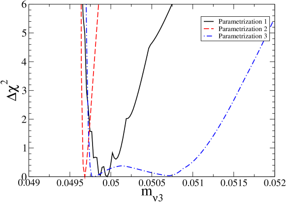
Figure 2: Predicted mass for the third generation neutrino using the same parametrization for both charged leptons and neutrinos.

In addition to the moduli of the CKM matrix, we have information of the angles $\alpha,\beta,\gamma$ which could include information of the phases that can be lost if we consider only the moduli of the CKM elements since

$$\alpha^{th} = {\rm arg}\left(-\frac{V_{cd}V_{cb}^{*}}{V_{td}V_{tb}^{*}}\right)$$ (18)

$$\beta^{th} = {\rm arg}\left(-\frac{V_{td}V_{tb}^{*}}{V_{ud}V_{ub}^{*}}\right)$$ (19)

$$\gamma^{th} = {\rm arg}\left(-\frac{V_{ud}V_{ub}^{*}}{V_{cd}V_{cb}^{*}}\right)\,.$$ (20)

The current values of the unitary angles are Nakamura et al. (2010):

$$\alpha^{Exp} = 89.0^{o}\pm 4.4^{o}$$

$$\beta^{Exp} = 21.15\pm 0.65^{o}$$

$$\gamma^{Exp} = 73^{o}\pm 22^{o}$$ (21)

On the other hand, the neutrino masses are not measured. Instead, the difference in masses have been obtained from the observation of solar, atmospheric, reactor and accelerator neutrinos. The current limits on the mass difference are

$$\Delta m_{12}^{2} = 7.67^{+0.22}_{-0.21}\times 10^{-5}{\rm eV}^{2}$$

$$\Delta m_{13}^{2} = 2.46\pm 0.15\times 10^{-3}{\rm eV}^{2}\quad({\rm normal\quad hierarchy})$$ (22)

and the determination of the mixing angles, including the latest result for a large lepton mixing angle $\theta_{13}$ provided by T2K, MINOS and Double Chooz experiments, gives updated values for $U_{\rm PMNS}$ Fogli et al. (2011):

$$U_{\rm PMNS}=\begin{pmatrix}0.824^{+0.011}_{-0.010}&0.547^{+0.016}_{-0.014}&0.145^{+0.022}_{-0.031}\\ 0.500^{+0.027}_{-0.021}&0.582^{+0.050}_{-0.023}&0.641^{+0.061}_{-0.023}\\ 0.267^{+0.044}_{-0.027}&0.601^{+0.048}_{-0.022}&0.754^{+0.052}_{-0.020}\,.\end{pmatrix}$$ (23)

With the the help of the definition of the theoretical mixing matrices (15) and the experimental values (17) we perform a simple $\chi^{2}$ analysis on the

$$\chi^{2}_{\rm quarks}(a_{u},a_{d},\phi)=\sum^{9}_{i=1}\left(\frac{V_{\rm CKM}^{th}(a_{u},a_{d},\phi)-|V_{\rm CKM}|}{\delta V_{\rm CKM}}\right)^{2}+\chi^{2}_{\rm angles}\,.$$ (24)

with

$$\chi^{2}_{\rm angles}=\left(\frac{\alpha^{th}-\alpha^{Exp}}{\delta\alpha^{Exp}}\right)^{2}+\left(\frac{\beta^{th}-\beta^{Exp}}{\delta\beta^{Exp}}\right)^{2}+\left(\frac{\gamma^{th}-\gamma^{Exp}}{\delta\gamma^{Exp}}\right)^{2}\,.$$ (25)

For the case of $U_{\rm PMNS}$, the $\chi^{2}$ is also a function of the mass of the heaviest neutrino $m_{\nu 3}$. For leptons we perform the $\chi^{2}$ analysis only with the moduli of the $U_{\rm PMNS}$ matrix

$$\chi^{2}_{\rm leptons}(a_{l},a_{\nu},\Phi_{1},m_{\nu 3})=\sum^{9}_{i=1}\left(\frac{U_{\rm PMNS}^{th}(a_{l},a_{\nu},\Phi_{1},m_{\nu 3})-|U_{\rm PMNS}|}{\delta U_{\rm PMNS}}\right)^{2}\,.$$ (26)

The results are summarized in Figs. 1, 2,3 and Table 1 and Table 2.

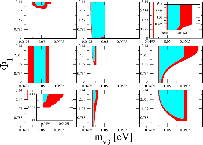
Figure 3: $m_{\nu 3}-\Phi_{1}$ allowed regions that fit $U_{\rm PMNS}$ for different choices in the parametrization for charged leptons and neutrinos. From left to right, and top to bottom: parametrization 1 for both, charged leptons and neutrinos, parametrization 1 for charged leptons and parametrization 2 for neutrinos, parametrization 1 for charged leptons and parametrization 3 for neutrinos and so on.

Parametrization	1	2	3
1	$\chi^{2}_{min}=930.02$	$\chi^{2}_{min}=3.55\times 10^{5}$	$\chi^{2}_{min}=3.55\times 10^{5}$
2	$\chi^{2}_{min}=1.43\times 10^{5}$	$\chi^{2}_{min}=1.270$	$\chi^{2}_{min}=2.212$
3	$\chi^{2}_{min}=4.50\times 10^{5}$	$\chi^{2}_{min}=1.44$	$\chi^{2}_{min}=2.163$

Table 1: The minimum value of $\chi^{2}_{\rm quarks}$. We can see that some parametrizations produces very big values $\chi^{2}_{\rm quarks}$, and so, they are ruled out as good parametrization

Fig. 1 shows the allowed values of $a_{u}^{\prime}$ and $a_{d}^{\prime}$ that reproduce the $V_{\rm CKM}$ matrix elements for different parametrization for $u$ and $d$-type quarks. Additionally, we can see from the minimum values of $\chi^{2}_{\rm quarks}$ reported in Table 1 that some parametrization are not able to allow us to reproduce $V_{\rm CKM}$ or the angles. That is the reason why only four different combinations are shown in Fig. 1.

On the other hand, for the case of neutrinos, the minimum $\chi^{2}_{\rm leptons}$ is reported in Table 2. It shows that the nine different combinations of parametrization for charged leptons and neutrinos give reasonable values of $\chi^{2}_{\rm leptons}$. Fig. 2 shows the projection in $m_{nu_{3}}$ of the neutrino mass for the case when the same parametrization for both charged leptons and neutrinos. Finally, Fig. 3 shows the projection in the plane $m_{\nu 3}-\Phi_{1}$ at 68% C.L. (cyan) and 90% C.L. (red).

Parametrization	1	2	3
1	$\chi^{2}_{min}=4.758$	$\chi^{2}_{min}=0.009$	$\chi^{2}_{min}=11.02$
2	$\chi^{2}_{min}=4.798$	$\chi^{2}_{min}=0.006$	$\chi^{2}_{min}=3.119$
3	$\chi^{2}_{min}=7.087$	$\chi^{2}_{min}=0.456$	$\chi^{2}_{min}=0.006$

Table 2: The minimum value of $\chi^{2}_{leptons}$. produces very big values $\chi^{2}_{quarks}$, contrary to the case of quarks, most of the parametrization give reasonable values of $\chi^{2}_{min}$

IV Conclusion

To conclude, we want to stress that this is a complete analysis for the four-zero textures in quark and leptonic sectors for no-hermitian Yukawa matrices made within a general formalism.In order to take into account the CP violation, one assumption has been done in order to simplify the inclusion of the CP violating phases in our analysis. This assumption corresponds to fix $\phi\equiv\phi^{u}_{1}-\phi^{d}_{1}=\phi^{u}_{2}-\phi^{d}_{2}$ and $\Phi_{1}\equiv\phi^{\ell}_{1}-\phi^{\nu}_{1}=\phi^{\ell}_{2}-\phi^{\nu}_{2}$ as defined in eq.(15). The diagonalization of the mass matrices has been obtained without introducing any more approximations. We analyse the different parametrizations of the four-zero texture mass matrices for quarks and leptons, that are able to reproduce the CKM and PMNS mixing matrices. It is important to stress that the relation between fermion masses and mixing angles obtained through our analysis are not the same as the ones usually given in Hermitian case where some approximation have been done in order to diagonalize the mass matrices Matsuda and Nishiura (2006) . This analysis is done through a $\chi^{2}$ analysis with up to date values of the mixing matrices and angles. In quark sector, only four solutions are found to be compatible with CKM mixing matrix. In leptonic sector, using the last experimental results about the mixing angles in the neutrino sector, our $\chi^{2}$ analysis shows a preferred value for $m_{\nu_{3}}$ to be around $0.05$ $eV$ independently of the parametrization of the four-zero texture mass matrices chosen for the charged leptons and neutrinos. This is a strong prediction for the four-zero texture models. This value for neutrino masses favors standard leptogenesis as the mechanism to produce the Baryon Asymmetry of the Universe Buchmuller et al. (2005). As expected, the leptonic $CP$ violating phases cannot be fixed through this analysis.