The Link Volume of 3-Manifolds

Abstract.

We view closed orientable 3-manifolds as covers of $S^{3}$ branched over hyperbolic links. For a cover $M\stackrel{{\scriptstyle p}}{{\to}}S^{3}$, of degree $p$ and branched over a hyperbolic link $L\subset S^{3}$, we assign the complexity $p\mbox{\rm Vol}(S^{3}\setminus L)$. We define an invariant of 3-manifolds, called the link volume and denoted $\mbox{\rm LinkVol}(M)$, that assigns to a 3-manifold $M$ the infimum of the complexities of all possible covers $M\to S^{3}$, where the only constraint is that the branch set is a hyperbolic link. Thus the link volume measures how efficiently $M$ can be represented as a cover of $S^{3}$.

We study the basic properties of the link volume and related invariants, in particular observing that for any hyperbolic manifold $M$, $\mbox{\rm Vol}(M)<\mbox{\rm LinkVol}(M)$. We prove a structure theorem (Theorem 1.1) that is similar to (and uses) the celebrated theorem of Jørgensen and Thurston. This leads us to conjecture that, generically, the link volume of a hyperbolic 3-manifold is much bigger than its volume (for precise statements see Conjectures 1.2 and 1.3).

Finally we prove that the link volumes of the manifolds obtained by Dehn filling a manifold with boundary tori are linearly bounded above in terms of the length of the continued fraction expansion of the filling curves (for a precise statement, see Theorem 1.6).

1. Introduction

The study of 3-manifolds as branched covers of $S^{3}$ has a long history. In 1920 Alexander [1] gave a very simple argument showing that every closed orientable triangulated 3-manifold is a cover of $S^{3}$ branched along the 1-skeleton of a tetrahedron embedded in $S^{3}$. We explain his construction and give basic definitions in Section 2. Clearly, if a 3-manifold $M$ is a finite sheeted branched cover of $S^{3}$, then $M$ is closed and orientable. Moise [16] showed that every closed 3-manifold admits a triangulation; thus we see: a 3-manifold $M$ is closed and orientable if and only if $M$ is a finite sheeted branched cover of $S^{3}$. From this point on, by manifold we mean connected closed orientable 3-manifold.

Alexander himself noticed one weakness of his theorem: the branch set is not a submanifold. He claimed that this can be easily resolved, but gave no indication of the proof. In 1986 Feighn [6] substantiated Alexander’s claim, Modifying the branch set to be a link.

Thurston showed the existence of a universal link, that is, a link $L\subset S^{3}$ so that every 3-manifold is a cover of $S^{3}$ branched along $L$. Hilden, Lozano and Montesinos [9] [10] drastically simplified Thurston’s example showing, in particular, that the figure eight knot is universal. Cao and Meyerhoff [4] showed that the figure eight knot is the hyperbolic link of smallest volume. In this paper, we consider hyperbolic links and consider their volume as a measure of complexity, hence we see that every 3-manifold is a cover of $S^{3}$, branched along the simplest possible link.

Our goal is to define and study invariant that asks: how efficient is the presentation of a 3-manifolds as a branched over of $S^{3}$? We do this as follows: let $M$ be a $p$-fold cover of $S^{3}$, branched along the hyperbolic link $L$. We denote this as $M\stackrel{{\scriptstyle p}}{{\to}}(S^{3},L)$ (read: $M$ is a $p$-fold cover of $S^{3}$ branched along $L$). The complexity of $M\stackrel{{\scriptstyle p}}{{\to}}(S^{3},L)$ is defined to be the degree of the cover times the volume of $L$, that is:

$$p\mbox{\rm Vol}(S^{3}\setminus L).$$

The link volume of $M$, denoted $\mbox{\rm LinkVol}(M)$, is the infimum of the complexities of all covers $M\stackrel{{\scriptstyle p}}{{\to}}(S^{3},L)$, subject to the constraint that $L$ is a hyperbolic link; that is:

$$\mbox{\rm LinkVol}(M)=\inf\{p\mbox{\rm Vol}(S^{3}\setminus L)|M\stackrel{{\scriptstyle p}}{{\to}}(S^{3},L)\,;\,L\mbox{ hyperbolic}\}.$$

Given a hyperbolic manifold $M$ we consider its volume, $\mbox{\rm Vol}(M)$, as its complexity. This is consistent with our attitude towards hyperbolic links, and is considered very natural by many 3-manifold topologists. Why is that? What is it that the volume actually measures? Combining results of Gromov, Jørgensen, and Thurston (for a detailed exposition see [11]) we learn the following. Let $t_{C}(M)$ denote the minimal number of tetrahedra required to triangulate a link exterior in $M$, that is, the least number of tetrahedra required to triangulate $M\setminus N(L)$, where the minimum is taken over all possible links $L\subset M$ (possibly, $L=\emptyset$) and all possible tringulations of $M\setminus N(L)$. Then there exist constants $a,b>0$ so that

(1) $$a\mbox{\rm Vol}(M)\leq t_{C}(M)\leq b\mbox{\rm Vol}(M).$$

We consider invariants up-to linear equivalence, and so we see that Vol and $t_{C}$ are equivalent. This gives a natural, topological interpretation of the volume. In this paper we begin the study of the link volume, with the ultimate goal of obtaining a topological understanding of it.

The basic facts about the link volume are presented in Section 4. The most important are the following easy observations:

1. The link volume is obtained, that is, for any manifold $M$ there is a cover $M\stackrel{{\scriptstyle p}}{{\to}}(S^{3},L)$ so that $\mbox{\rm LinkVol}(M)=p\mbox{\rm Vol}(S^{3}\setminus L)$.

2. For every hyperbolic 3-manifold $M$ we have:

   $$\mbox{\rm Vol}(M)<\mbox{\rm LinkVol}(M).$$

The second point begs the question: is the link volume of hyperbolic manifolds equivalent to the hyperbolic volume? As we shall see below, the results of this paper lead us to believe that this is not the case (Conjectures 1.2 and 1.3).

The right hand side of the Inequality (1) implies that, for fixed $V$, any hyperbolic manifold of volume less than $V$ can be obtained from a manifold $X$ by Dehn filling, where $X$ is constructed using at most $bV$ tetrahedra. Since there are only finitely many such $X$’s, this implies the celebrated result of Jørgensen–Thurston: for any $V>0$, there exists finite collection of compact “parent manifolds” $\{X_{i},\dots X_{n}\}$, so that $\partial X_{i}$ consists of tori, and any hyperbolic manifold of volume at most $V$ is obtained by Dehn filling $X_{i}$, for some $i$. Our first result is:

Theorem 1.1.

There exists a universal constant $\Lambda>0$ so that for every $V>0$, there is a finite collection $\{\phi_{i}:X_{i}\to E_{i}\}_{i=1}^{n_{V}}$, where $X_{i}$ and $E_{i}$ are complete finite volume hyperbolic manifolds and $\phi_{i}$ is an unbranched cover, and for any cover $M\stackrel{{\scriptstyle p}}{{\to}}(S^{3},L)$ with $p\mbox{\rm Vol}(S^{3}\setminus L)<V$ the following hold:

1. For some $i$, $M$ is obtained from $X_{i}$ by Dehn filling, $S^{3}$ is obtained from $E_{i}$ by Dehn filling, and the following diagram commutes (where the vertical arrows represent the covering projections and the horizontal arrows represent Dehn fillings):

2. $E_{i}$ can be triangulated using at most $\Lambda V/p$ tetrahedra (hence $X_{i}$ can be triangulated using at most $\Lambda V$ tetrahedra and $\phi_{i}$ is simplicial).

For $V>0$, let $\mathcal{M}_{V}$ denote the set of manifolds of link volume less than $V$. Since the link volume is always obtained, applying Theorem 1.1 to covers realizing the link volumes of manifolds in $\mathcal{M}_{V}$, we obtain a finite family of “parent manifolds” $X_{1},\dots,X_{n}$ that give rise to every manifold in $\mathcal{M}_{V}$ via Dehn filling, much like Jørgensen–Thurston. The extra structure given by the projection $\phi_{i}:X_{i}\to E_{i}$ implies that the fillings that give rise to manifolds of low link volume are very special:

Fix $V$, and let $X_{i}$ be as in the statement of Theorem 1.1. Then for any hyperbolic manifold $M$ that is obtained by filling $X_{i}$ we have $\mbox{\rm Vol}(M)<\mbox{\rm Vol}(X_{i})$. On the other hand, it is by no means clear that $\mbox{\rm LinkVol}(M)<V$, for it is not easy to complete the diagram in Theorem 1.1:

1. $X_{i}$ must cover a manifold $E_{i}$.

2. The covering projection and the filled slopes must be compatible (see Subsection 2.3 for definition).

3. The slopes filled on $E_{i}$ must give $S^{3}$, a very unusual situation since $E_{i}$ is hyperbolic.

These lead us to believe that the link volume, as a fuction, is much bigger than the volume. Specifically we conjecture:

Conjecture 1.2.

Let $X$ be a complete finite volume hyperbolic manifold with one cusp. For a slope $\alpha$ on $\partial X$, let $X(\alpha)$ denote the closed manifold obtained by filling $X$ along $\alpha$.

Then for any $V>0$, there exists a finite set of slopes $\mathcal{F}$ on $\partial X$, so that if $\mbox{\rm LinkVol}(X(\alpha))<V$, then $\alpha$ intersects some slope in $\mathcal{F}$ at most $V/2$ times.

As is well known, the volume of the figure eight knot complement is about $2.029\dots$, twice $v_{3}$, the volume of a regular ideal tetrahedron. By considering manifolds that are obtained by Dehn filling the figure eight knot exterior we see that Conjecture 1.2 implies:

Conjecture 1.3.

For every $V>0$ there exists a manifold $M$ so that $\mbox{\rm Vol}(M)<2v_{3}=2.029\dots$ and $\mbox{\rm LinkVol}(M)>V$.

To describe our second result, we first define the knot volume and a few other variations of the link volume; for the definition simple cover see the Subsection 2.2.

Definitions 1.4.

1. The knot volume of a 3-manifold $M$ is obtained by considering only hyperbolic knots in the definition of the link volume, that is,

   $$\mbox{\rm KnotVol}(M)=\inf\{p\mbox{\rm Vol}(S^{3}\setminus K)|M\stackrel{{\scriptstyle p}}{{\to}}(S^{3},K);K\mbox{ is a hyperbolic knot}\}.$$

2. The simple knot volume of a 3-manifold $M$ is obtained by considering only simple covers in the definition of the knot volume, that is,

   $$\mbox{\rm KnotVol}_{s}(M)=\inf\left\{p\mbox{\rm Vol}(S^{3}\setminus K)\Bigg{|}M\stackrel{{\scriptstyle p}}{{\to}}(S^{3},K);\begin{array}[]{l}K\mbox{ a hyperbolic knot},\\ \mbox{and the cover is simple}\end{array}\right\}.$$

3. For an integer $d\geq 3$, the simple $d$-knot volume in obtained by restricting to $p$-fold covers for $p\leq d$ in the definition of the simple knot volume, that is,

   $$\mbox{\rm KnotVol}_{s,{d}}(M)=\inf\left\{p\mbox{\rm Vol}(S^{3}\setminus K)\Bigg{|}M\stackrel{{\scriptstyle p}}{{\to}}(S^{3},K);\begin{array}[]{l}K\mbox{ a hyperbolic knot},\\ \mbox{the cover is simple},\\ \mbox{and }p\leq d\end{array}\right\}.$$

Similarly, one can play with various restrictions on the covers considered. However, one must ensure that the definition makes sense. For example, the regular link volume can be defined using only regular covers. This makes no sense, as not every manifold is the regular cover of $S^{3}$. It follows from Hilden [8] and Montesinos [17] that every 3-manifold is a simple 3-fold cover of $S^{3}$ branched over a hyperbolic knot; hence the definitions above make sense. Our next result is an upper bound, and holds for any of the variations listed in Definitions 1.4. Since these definitions are obtained by adding restrictions to the covers considered, it is clear that $\mbox{\rm KnotVol}_{s,{3}}(M)$ is greater than or equal to any of the others, including the link volume. We therefore phrase Theorem 1.6 below for that invariant. But first we need:

Definition 1.5.

Let $T$ be a torus, and $\mu$, $\lambda$ generators for $H_{1}(T)$. By identifying $\mu$ with $1/0$ and $\lambda$ with $0/1$, we get an identification of the slopes of $H_{1}(T)$ with $\mathbb{Q}\cup\{1/0\}$, where an element of $H_{1}(T)$ is called a slope if it can be represented by a connected simple closed curve on $T$. Then the depth of a slope $\alpha$, denoted $\mbox{\rm depth}(\alpha)$, is the length of the shortest contiuded fraction expenssion representing $p/q$. For a collection of tori $T_{1},\dots,T_{n}$ with bases chosen for $H_{1}(T_{i})$ for each $i$, we define

$$\mbox{\rm depth}(p_{1}/q_{1},\dots,p_{n}/q_{n})=\Sigma_{i=1}^{n}\mbox{\rm depth}(p_{i}/q_{i}).$$

We are now ready to state:

Theorem 1.6.

Let $X$ be a connected, compact orientable $3$-manifold, $\partial X$ consisting of $n$ tori $T_{1},\dots,T_{n}$, and fix $\mu_{i}$, $\lambda_{i}$, generators for $H_{1}(T_{i})$ for each $i$.

Then there exist a universal constant $B$ and a constant $A$ that depends on $X$ and the choice of bases for $H_{1}(T_{i})$, so that for any $p_{i}/q_{i}$ ($i=1,\dots,n$),

$$\mbox{\rm KnotVol}_{s,{3}}(X(p_{1}/q_{1},\dots,p_{n}/q_{n}))<A+B\mbox{\rm depth}(p_{1}/q_{1},\dots,p_{n}/q_{n}),$$

where $X(p_{1}/q_{1},\dots,p_{n}/q_{n})$ denotes the manifold obtained by filling $X$ along the slopes $p_{i}/q_{i}$.

As noted above, $\mbox{\rm KnotVol}_{s,{3}}(M)$ is greater than or equals to all the invariants defined in Definition 1.5 and the link volume. Hence Theorem 1.6, which gives an upper bound, holds for all these invariants, and in particular:

Corollary 1.7.

With the hypotheses of Theorem 1.6, there exist a universal constant $B$ and a constant $A$ that depends on $X$ and the choice of bases for $H_{1}(T_{i})$, so that for any slopes $p_{i}/q_{i}$ ($i=1,\dots,n$),

$$\mbox{\rm LinkVol}(X(p_{1}/q_{1},\dots,p_{n}/q_{n}))\leq A+B\mbox{\rm depth}(p_{1}/q_{1},\dots,p_{n}/q_{n}).$$

Organization. This paper is organized as follows. In Section 2 we go over necessary background material. In Section 3 we explain some possible variation on the link volume. Notably, we define the surgery volume (definition due to Kimihiko Motegi) and an invariant denote $pB(M)$ (definition due to Ryan Blair). We show that ,in contrast to the link volume, the surgery volume of hyperbolic manifolds is bounded in terms of their volume. We also show that $pB(M)$ is linearly equivalent to $g(M)$, the Heegaard genus of $M$. In Section 4 we explain basic facts about the link volume and list some open questions. In Section 5 we prove Theorem 1.1. In Section 6 we prove Theorem 1.6.

Acknowledgement. We thank Ryan Blair, Tsuyoshi Kobayashi, Kimihiko Motegi, Hitoshi Murakami, and Jair Remigio–Juárez for helpful conversations.

2. Background

By manifold we mean connected, closed, orientable 3-manifold. In some cases, we consider connected, compact, orientable 3-manifolds; then we explicitly say compact manifold. By hyperbolic manifold $X$ we mean a complete, finite volume Riemannian 3-manifold locally isometric to $\mathbb{H}^{3}$. It is well know that any hyperbolic manifold $X$ is the interior of a compact manifold $\bar{X}$ and $\bar{X}\setminus X=\partial\bar{X}$ consists of tori. To simplify notation, we do not refer to $\bar{X}$ explicitly and call $\partial\bar{X}$ the boundary of $X$. We assume familiarity with the basic concepts of 3-manifold theory and hyperbolic manifolds, and in particular the Margulis constant. By volume we mean the hyperbolic volume. The volume of a hyperbolic manifold $M$ is denoted $\mbox{\rm Vol}(M)$.

We follow standard notation. In particular, by Dehn filling (or simply filling) we mean attaching a solid torus to a torus boundary component.

2.1. Branched covering

We begin by recalling Alexander’s Theorem [1]; because this theorem is very short an elegant, we include a sketch of its proof here.

Theorem 2.1 (Alexander).

Let $\mathcal{T}$ be a triangulation of $S^{n}$ obtained by doubling an $n$-simplex. Let $M$ be a closed orientable triangulated $n$-manifold. Then $M$ is a cover of $S^{n}$ branched along $\mathcal{T}^{(n-2)}$, the $n-2$-skeleton of $\mathcal{T}$.

Sketch of Proof.

Let $M$ be as above. Given $\mathcal{T}_{M}$, a triangulation of $M$, let $\mathcal{T^{\prime}}_{M}$ denote its barycentric subdivision. Each vertex $v$ of $\mathcal{T}_{M}^{\prime}$ is the center of a $k$-face of $\mathcal{T}_{M}$, for some $k$. Label $v$ with the label $k$. By construction, there are exactly $n+1$ labels, $0,\dots,n$, and no two adjacent vertices have the same label.

Note that the 1-skeleton of $\mathcal{T}$ is $K_{n+1}$, the complete graph on $n+{1}$ vertices. Label these vertices with the labels $0,\dots,n$ so that every label appears exactly once.

We define a function from $\mathcal{T}_{M}^{\prime(n-1)}$ (the $n-1$ skeleton of $\mathcal{T}_{M}^{\prime}$) to $S^{n}$ by sending each $k$-face simplicially to the unique $k$-face of $S^{n}$ with the same labeling (for $k<n$); it is easy to see that this function is well defined. However, the $n$-cells of $M$ can be sent to either of the two $n$ simplices of $\mathcal{T}_{M}^{\prime}$. We pick the simplex so that the map is orientation preserving.

It is left to the reader to verify that this is indeed a cover, branched over the $n-2$ skeleton of the triangulation of $S^{n}$. ∎

Lemma 2.2.

For any compact triangulated $n$-manifold $M$, $B\subset M^{(n-2)}$ a subcomplex, and $d>0$, there are only finitely many $d$-fold covers of $M$ branched along $B$.

Proof.

It is well known that a $p$-fold cover of $M$ branched along $B$ is determined by a presentation of $\pi_{1}(M\setminus B)$ into $S_{p}$, the symmetric group on $p$ elements (see, for example, [22]). The lemma follows from the fact that $\pi_{1}(M\setminus B)$ is finitely generated and $S_{p}$ is finite. ∎

2.2. Simple covers and the Montesinos Move

Definition 2.3.

Let $f:M\to N$ be a cover of finite degree $p$ branched along $B\subset N$. Note that every point of $N\setminus B$ has exactly $p$ preimages, and every point of $B$ has at most $p$ preimages. $f:M\to N$ is called simple if every point of $B$ has exactly $p-1$ preimages.

Let $M\to(S^{3},L)$ be a 3-fold simple cover branched along the link $L$. We view $L$ diagrammatically, as projected into $S^{2}\subset S^{3}$ in the usual way. Since the cover is simple, each generator in the Wirtinger presentation of $S^{3}\setminus L$ corresponds to a permutation in the symmetric group on 3 elements (that is, $(1\ 2)(3)$ or $(1\ 3)(2)$ or $(2\ 3)(1)$). We consider these as three colors, and color each strand of $L$ accordingly. By assumption, $M$ is connected; hence not all generators correspond to the same permutation. Finally, the relators of the Wirtinger presentation guarantee that at each crossing wither all three color appear, or only one color does. Thus we obtain a 3 coloring of the strands of $L$.

Montesinos proved that if we replace a positive crossing where all three colors appear by 2 negative crossings the cover is not changed. This is called the Montesinos move. The reason is simple: the neighborhood of a 3-colored crossing is a ball, and its cover is a ball as well. (This is false if only one color appears at the crossing!) More generally, when all three colors appear we can replace $n$ half twists with $n+3k$ half twists ($n,k\in\mathbb{Z}$). The case $n=0$ is allowed, but then we must require that the two strands in question have distinct colors. We denote such a move by $n\mapsto n+3k$ Montesinos move. In Figure 1 we show a few views of the Montesinos Move.

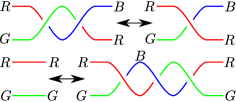
Figure 1. Montesinos move

Finally, we record the following fact for future reference. It is easy to see that the $p$-fold cover cover $f:M\to S^{3}$ branched along $B\subset S^{3}$ is connected if and only if the image of $\pi_{1}(S^{3}\setminus B)$ in $S_{p}$ acts transitively on the set f $p$ letters. For simple 3-fold covers this means:

Lemma 2.4.

Let $M$ be a 3-manifold and $f:M\to S^{3}$ a simple 3-fold cover branched along the link $L\subset S^{3}$. Then $M$ is connected if and only if at least two colors appear in the 3-coloring of $L$.

2.3. Slopes on tori and coverings

Recall that s slope on a torus is the free homotopy class of a connected simple closed curve, up to reserving the orientation of the curve. For this subsection we fix the following: let $X$ and $E$ be complete hyperbolic manifolds of finite volume, and $\phi:X\to E$ an unbranched cover. Let $T$ be a boundary component of $X$; note that $\phi$ induces an unbranched cover $T\to\phi(T)$.

Let $\alpha$ be a slope on $T$ realized by a connected simple closed curve $\gamma\subset T$. Then $\phi(\gamma)$ is a (not necessarily simple) connected essential curve on $\phi(T)$. Since $\phi(T)$ is a torus, there is a curve $\bar{\beta}$ on $\phi(T)$ so that $\phi(\gamma)$ is homotopic to $\bar{\beta}^{m}$, for some $m\neq 0$. Let $\beta$ be the slope defined by $\bar{\beta}$. Define the function $\phi_{\downarrow}$ from the slopes on $T$ to the slopes on $\phi(T)$ by setting $\phi_{\downarrow}(\alpha)=\beta$.

Conversely, let $\alpha$ be a slope on $\phi(T)$ realized by a connected simple closed curve $\gamma\subset\phi(T)$. Then $\phi^{-1}(\gamma)$ is a (not necessarily connected) essential simple closed curve. Each component of $\phi^{-1}(\gamma)$ defines a slope on $T$, and since these curves are disjoint, they all define the same slope, say $\beta$. Define the function $\phi_{\uparrow}$ from the slopes on $\phi(T)$ to the slopes on $T$ by setting $\phi_{\uparrow}(\alpha)=\beta$. It is easy to see that $\phi_{\downarrow}$ is the inverse of $\phi_{\uparrow}$. We say that $\alpha$ and $\phi_{\downarrow}(\alpha)$ are corresponding slopes.

Suppose that we Dehn fill $T$ and $\phi(T)$. If the slope filled are not corresponding, then the curve filled on $T$ maps to a curve of $\phi(T)$ that is not null homotopic in the attached solid torus. Thus the map $\phi$ cannot be extended into that solid torus.

Conversely, suppose that corresponding slopes are filled. We parametrize the attached solid tori as $S^{1}\times D^{2}$, and extend $\phi$ into the solid tori by coning along each disk $\{p\}\times D^{2}$ ($p\in S^{1}$). It is easy to see that the extended map is a cover, branched (if at all) along the core of the attached solid torus. (The local degree at the core of the solid torus is the number denoted by $m$ in the construction of $\phi_{\downarrow}$ above.)

In conclusion, $\phi$ induces a correspondence between slopes of $T$ and slopes on $\phi(T)$, and $\phi$ can be extended to the attached solid tori to give a branched cover after Dehn filling if and only if corresponding slopes are filled.

Next, let $T_{1}$, $T_{2}\subset\partial X$ be tori that project to the same component of $\partial E$. Then two bijections $\phi_{\downarrow}$ from the slopes of $T_{1}$ and $T_{2}$ to the slopes of $\phi(T_{1})=\phi(T_{2})$ induce a bijection between the slopes of $T_{1}$ and the slopes of $T_{2}$; again we call slopes that are interchanged by this bijection corresponding. Filling $T_{1}$ and $T_{2}$ along corresponding slopes is called consistent, inconsistent otherwise. Note that after filling $X$ there is a filling of $E$ so that the cover $X\to E$ extends to a branched cover if and only if the filling of $X$ is consistent on every pair of components of $\partial X$.

2.4. Hyperbolic alternating links

In this subsection we follow Chapter 4 of Lickorish [14]. We begin with the following standard definitions:

Definitions 2.5.

Let $L$ be a link and $D$ a diagram for $L$. The projection sphere is denoted $S^{2}$. Then $D$ is called alternating if, for each component $K$ of $L$, when traversing the projection of $K$ the crossing occur as …over, under, over, under,…. $L$ is called an alternating link if it admits an alternating diagram. A link diagram $D$ is called strongly prime if any simple closed curve that intersects it transversely in two simple points (that is, two points that are not crossings) bounds a disk that $D$ intersects in a single arc with no crossings. A link $L$ is called split if its exterior admits an essential sphere, that is, if there is an embedded sphere $S\subset S^{3}\setminus L$ so that each of the balls obtained by cutting $S^{3}$ open along $S$ contains at least one component of $L$. A link diagram $D\subset S^{2}$ is called a split diagram if there is a circle $\gamma$ embedded in $S^{2}$, so that each disk obtained by cutting $S^{2}$ open along $\gamma$ contains at least one component of $D$. Note that a split diagram is necessarily a diagram for a split link, but the converse does not hold. A link is called simple if its exterior does not admit an essential surface of non-negative Euler characteristic. A link $L$ is called hyperbolic if $S^{3}\setminus L$ admits a complete, finite volume, hyperbolic metric.

Menasco ([15], see also [14]) proved:

Theorem 2.6.

Let $D$ be an alternating link diagram for a link $L$. If $D$ is strongly prime and is not split, then $L$ is simple.

Thurston proved:

Theorem 2.7.

Any simple link is hyperbolic.

Combining these results, we obtain:

Corollary 2.8.

If a link $L$ has a non-split, strongly prime, alternating diagram, then $L$ is hyperbolic.

2.5. Twist number and hyperbolic volume

For the definition of twist number see, for example, [13]. We briefly recall it here. Let $D$ be a link diagram. Let $\sim$ be the equivalent relation on the crossings of $D$ generated by $c\sim c^{\prime}$ if $c$ and $c^{\prime}$ lie on the boundary of a bigon of $D$. This equivalence relation can be visualized as follows: if $c_{1},\dots,c_{n}$ form an equivalence class of crossings, then after reordering them if necessary, there is a chain of $n-1$ bigons in $D$ with $c_{i-1}$ and $c_{i}$ on the boundary the $i$th bigon.

The twist number of a link $L$, denoted $t(L)$, is the smallest number of equivalence classes in any diagram for $L$. Thus, for example, the obvious diagram of twist knots show they have twist number at most 2.

Lackenby [13] gave upper and lower bounds on the hyperbolic volume of link exteriors in terms of their twist number. We emphasize that the lower bound holds for alternating links (or, more precisely, for alternating diagrams), while the upper bound holds for all links. It is the upper bound that we will need in this work, hence we need not assume the diagram alternates. We will need:

Theorem 2.9 (Lackenby [13]).

There exists a constant $c$ so that for any hyperbolic link $L$,

$$\mbox{\rm Vol}(S^{3}\setminus L)\leq ct(L).$$

3. Variations

In this section we discuss two variations of the link volume. The first variation is obtained by replacing the volume by another knot invariant (note that one can use any invariant with values in $\mathbb{R}_{\geq 0}$). This variation was suggested by Ryan Blair. Let $L\subset S^{3}$ be a link and let $b(L)$ denote its bridge index. We consider the complexity of $M\stackrel{{\scriptstyle p}}{{\to}}(S^{3},L)$ to be $pb(L)$. Define $\mbox{pB}(M)$ to be the infimum of $pb(L)$, taken over all possible covers.

It is easy to see that the preimage of a bridge surface $S$ for $L$ is a Heegaard surface for $M$, say $\Sigma$. Since $S$ is a $2b$ punctured sphere, $\chi(S\setminus L)=2-2b$. Its preimage has Euler characteristic $p(2-2b)$. We obtain $\Sigma$ by adding some number of points, say $n\geq 0$. Then $\chi(\Sigma)=p(2-2b)+n$. Thus we get:

$$2g(\Sigma)-2 = -\chi(\Sigma)$$

$$= p(2b-2)-n$$

$$= 2pb-(2p+n)$$

$$\leq 2pb-2.$$

Since $\mbox{pB}(M)$ is positive integer valued, the infimum is obtained. By considering a cover that realizes $\mbox{pB}(M)$, we obtain a surface $\Sigma$ so that $g(\Sigma)\leq\mbox{pB}(M)$. Thus $g(M)\leq g(\Sigma)\leq\mbox{pB}(M)$.

The converse is highly non-trivial. Given an arbitrary manifold $M$, Hilden [8] constructed a $3$-fold cover $M\stackrel{{\scriptstyle 3}}{{\to}}(S^{3},L)$. The construction uses an arbitrary Heegaard surface $\Sigma\subset M$. One feature of Hilden’s construction is that $b(L)\leq 2g(\Sigma)+2$. Since $\Sigma$ was an arbitrary Heegaard surface, we may assume that $g(\Sigma)=g(M)$. Thus we see that $\mbox{pB}(M)\leq 6g(M)+6$. Combining the inequalities we got we obtain:

$$g(M)\leq\mbox{pB}(M)\leq 6g(M)+6.$$

Thus we see that the Heegaard genus and pB are equivalent.

Another variation, suggested by Kimihiko Motegi, is the surgery volume. Given a manifold $M$, it is well known that $M$ is obtained by Dehn surgery on a link in $S^{3}$, say $L$. By Myers  [19], every compact 3-manifold admits a simple knot. Applying this to $S^{3}\setminus N(L)$ we obtain a knot $K$ so that $L^{\prime}=L\cup K$ is a hyperbolic link. Since $M$ is obtained from $S^{3}$ via surgery along $L^{\prime}$ (with the original surgery coefficients on $L$ and the trivial slope on $K$), we conclude that $M$ is obtained from $S^{3}$ via surgery along a hyperbolic link. The surgery volume of $M$ is then

$$\mbox{SurgVol}(M)=\inf\{\mbox{\rm Vol}(S^{3}\setminus L)|M\mbox{ is obtained by surgery on }L,L\mbox{ is hyperbolic}\}.$$

Neumann and Zagier [20] showed that if a hyperbolic manifold $N_{1}$ is obtained by filling a hyperbolic manifold $N_{2}$, then $\mbox{\rm Vol}(N_{1})<\mbox{\rm Vol}(N_{2})$. Applying this in our setting (with $S^{3}\setminus L^{\prime}$ as $N_{1}$ and $M$ as $N_{2}$) we see that for any hyperbolic manifold $M$, $\mbox{\rm Vol}(M)\leq\mbox{SurgVol}(M).$

We note that there exists a function $f:(0,\infty)\to(0,\infty)$ so that any hyperbolic manifold $M$ is obtained by surgery on a hyperbolic link $L\subset S^{3}$ with $\mbox{\rm Vol}(S^{3}\setminus L)\leq f(\mbox{\rm Vol}(M))$. To see this, fix $V$ and let $X_{1},\dots,X_{n}$ be the set of parent manifolds of all hyperbolic manifolds of volume at most $V$. For each $X_{i}$ there is a link $L_{i}$ in $S^{3}$, so that $X_{i}$ is obtained by surgery on some of the components of $L_{i}$ and drilling the rest. Therefore, any hyperbolic manifold $M$ with volume at most $V$ is obtained on surgery on some $L_{i}$ ($i=1,\dots,n$). Set

$$f(V)=\max_{i=1}^{n}\{\mbox{\rm Vol}(S^{3}\setminus L_{i})\}.$$

We get:

$$\mbox{\rm Vol}(M)\leq\mbox{SurgVol}(M)\leq f(\mbox{\rm Vol}(M)).$$

The surgery volume and the hyperbolic volume are equivalent if there is a linear function $f$ as above; we do not know if this is the case.

4. Basic facts and open questions

Basic facts about the Link Volume:

The link volume is obtained:

that is, for every $M$ there exists a cover $M\stackrel{{\scriptstyle p}}{{\to}}(S^{3},L)$ so that $\mbox{\rm LinkVol}(M)=p\mbox{\rm Vol}(S^{3}\setminus L)$. Recall that the link volume was defined as an infimum. To see that there is a cover realizing it, we need to show that the infimum is obtained. Fix a manifold $M$, and let $M\stackrel{{\scriptstyle p_{n}}}{{\to}}(S^{3},L_{n})$ be a sequence of covers that approximates $\mbox{\rm LinkVol}(M)$. By Cao–Meyerhoff [4], for every $n$, $\mbox{\rm Vol}(S^{3}\setminus L_{n})>2$. Hence for large enough $n$, $p_{n}\leq\mbox{\rm LinkVol}(M)/2$; we see that there are only finitely many values for $p_{n}$. For any collection of covers $M\stackrel{{\scriptstyle d}}{{\to}}(S^{3},L_{i}^{\prime})$ of fixed degree $d$, the infimum of $\{d\mbox{\rm Vol}(S^{3}\setminus L_{i}^{\prime})\}$ is obtained, since the set of hyperbolic volumes is well-ordered. It follows that the link volume is realized by some cover in $\{M\stackrel{{\scriptstyle p_{n}}}{{\to}}(S^{3},L_{n})\}$.

The link volume is the volume of a link exterior:

that is, for any $M$, there exists $\widetilde{L}\subset M$ so that $\mbox{\rm LinkVol}(M)=\mbox{Vol}(M\setminus\widetilde{L})$. This follows easily from the previous point. Let $M\stackrel{{\scriptstyle p}}{{\to}}(S^{3},L)$ be a cover realizing the link volume. Let $\widetilde{L}$ be the preimage of $L$. Then the cover $M\to S^{3}$ induces a cover $M\setminus\widetilde{L}\to S^{3}\setminus L$. Since the cover $M\setminus\widetilde{L}\to S^{3}\setminus L$ is not branched, we can lift the hyperbolic structure on $S^{3}\setminus L$ to $M\setminus\widetilde{L}$. We obtain a complete finite volume hyperbolic structure on $M\setminus\widetilde{L}$ of volume $p\mbox{\rm Vol}(S^{3}\setminus)L=\mbox{\rm LinkVol}(M)$.

The link volume is bigger than the volume:

If $M$ is hyperbolic then $\mbox{\rm Vol}(M)<\mbox{\rm LinkVol}(M)$: this follows immediately from the previous point and the fact the volume always goes down under Dehn filling [20].

The spectrum of link volumes is well ordered:

it follows from the second point above that the spectrum of link volumes is a subset of the spectrum of hyperbolic volumes. Since the spectrum of hyperbolic volumes is well ordered, so are all of its subsets.

The spectrum of link volumes is ”small”:

the reader can easily make sense of the claim the the spectrum of link volumes is a very small subset of the spectrum of hyperbolic volume. In fact, the spectrum of link volumes is a subset of the spectrum integral products of volumes of hyperbolic links in $S^{3}$. However, it is not too small: there are infinitely many manifolds $M$ with $\mbox{\rm LinkVol}(M)<7.22\dots$. Moreover, in [21] Jair Remigio-Juarez and the first named author showed that there are infinitely many manifold of the same link volume, just under $7.22\dots$. This is in sharp contrast to the hyperbolic volume function which is finite-to-one.

For the remainder of this paper we will often use these facts without reference.

Basic questions about the Link Volume include:

1. Calculate $\mbox{\rm LinkVol}(M)$. It is not clear whether or not there exists an algorithm to calculate the link volume of a given manifold $M$. This would involves some questions about the set of links in $S^{3}$ that give rise to $M$ and appears to be quite hard.

2. The following question was proposed by Hitoshi Murakami: if $N\stackrel{{\scriptstyle q}}{{\to}}M$ is an unbranched cover then $\mbox{\rm LinkVol}(N)\leq q\mbox{\rm LinkVol}(M)$. How good is this bound? Even for $q=2$, the answer is not clear.

3. Since the link volume is obtained, for every manifold $M$ there is a positive integer $d$ which is the smallest integer so that there exists a cover $M\stackrel{{\scriptstyle d}}{{\to}}(S^{3},L)$ realizing $\mbox{\rm LinkVol}(M)$. What is $d$ and how does it reflect the topology of $M$? Can $d$ be arbitrarily large? Is any positive integer $d$ for some $M$?

4. Characterize the set $\{\widetilde{L}\subset M|\exists M\to S^{3}$, branched over $L$, and $\widetilde{L}$ is the preimage of $L\}$. The link volume is, of course, the minimal volume of the manifolds in this set, and in this paper we concentrate on it. It is easy to see that there is no upper bound to the volumes of manifolds in this set. It may be interesting to try and characterize the elements of this set.

5. Do there exist hyperbolic manifolds $M_{1}$, $M_{2}$ with $\mbox{\rm Vol}(M_{1})=\mbox{\rm Vol}(M_{2})$ and $\mbox{\rm LinkVol}(M_{1})\neq\mbox{\rm LinkVol}(M_{2})$?

6. Similarly, do there exist hyperbolic manifolds $M_{1}$, $M_{2}$ with $\mbox{\rm LinkVol}(M_{1})=\mbox{\rm LinkVol}(M_{2})$ and $\mbox{\rm Vol}(M_{1})\neq\mbox{\rm Vol}(M_{2})$? We note that the examples of manifolds with the same link volume mentioned above are all Siefert fibered spaces.

5. Proof of Theorem 1.1

Fix $V>0$. Fix $\mu>0$ a Margulis constant for $\mathbb{H}^{3}$ and $d>0$. (We remark that the constant $\Lambda$ that we obtain in this proof depends on these choices.)

Let $M$ be a manifold of $\mbox{\rm LinkVol}(M)<V$. Let $M\stackrel{{\scriptstyle p}}{{\to}}(S^{3},L)$ be a cover realizing $\mbox{\rm LinkVol}(M)$. Denote the $d$ neighborhood of the $\mu$-thick part of $S^{3}\setminus L$ by $E_{L}$. By construction, $E_{L}$ is obtained from $S^{3}\setminus L$ by drilling out certain geodesics; by Kojima [12, Proposition 4], $E_{L}$ is hyperbolic.

Let $X_{\phi}$ denote the preimage of $E_{L}$ in $M$. Then the cover $\phi:M\to S^{3}$ induces an unbranched cover $\phi:X_{\phi}\to E_{L}$. By lifting the hyperbolic structure from $E_{L}$ to $X_{\phi}$, we see that $X_{\phi}$ is a finite volume hyperbolic manifold.

By construction, the following diagram commutes (where vertical arrows represent the covering projections and horizontal arrows represent Dehn fillings):

By Jørgensen and Thurston (see, for example, [11]), there exists a constant $\Lambda$ (depending on $\mu$ and $d$), so that for any complete, finite volume hyperbolic manifold $N$, the $d$-neighborhood of the $\mu$-thick part of $N$ can be triangulated using no more than $\Lambda\mbox{\rm Vol}(N)$ tetrahedra. Applying this to $N=S^{3}\setminus L$, since the $d$-neighborhood of the $\mu$-thick part of $N$ is $E_{L}$, we see that $E_{L}$ can be triangulated using at most $\Lambda\mbox{\rm Vol}(S^{3}\setminus L)=\Lambda\mbox{\rm LinkVol}(M)/p<\Lambda V/p$ tetrahedra.

Since there are only finite many manifolds that can be triangulated using at most $\Lambda V/p$ tetrahedra, there are only finitely many possibilities for $E_{L}$.

Lifting the triangulation from $E_{L}$ to $X_{\phi}$, we see that $X_{\phi}$ can be triangulated with at most $\Lambda\mbox{\rm LinkVol}(M)<\Lambda V$ tetrahedra, and that $\phi:X_{\phi}\to E_{L}$ is simplicial. This shows that there are only finitely many possibilities for $X_{\phi}$ and $\phi$. We denote them $\{\phi_{i}:X_{i}\to E_{i}\}_{i=1}^{n_{V}}$.

6. The Link Volume and Dehn Filling

In this section we prove Theorem 1.6. The proof is constructive and requires two elements, the first is Hilden’s construction of simple 3-fold covers of $S^{3}$, and the second is the results of Thurston and Menasco that show that an alternating link that “looks like” a hyperbolic link is in fact hyperbolic. For the latter, see Subsection 2.4. We now explain the former.

In [8], Hilden showed that any 3-manifold is the simple 3-fold cover of $S^{3}$. The crux of his proof is the construction, for any $g$, of a 3-fold branched cover $p:V_{g}\to B$, where $V_{g}$ is the genus $g$ handlebody and $B$ is the 3-ball. He then proves that any map $f:\partial V_{g}\to\partial V_{g}$ can be isotoped so as to commute with $p$. Thus $f$ induces a map $\bar{f}:\partial B\to\partial B$ so that the following diagram commutes (here the vertical arrows denote Hilden’s covering projection):

Starting with a closed, orientable, connected 3-manifold $M$, Hildens uses a Heegaard splitting of $M=V_{g}\cup_{f}V_{g}$; the construction above gives a map to $B\cup_{\bar{f}}B\cong S^{3}$. This is, in a nutshell, Hilden’s construction of $M$ as a cover of $S^{3}$.

Our goal is using a similar construction to get a map from $X$. Since $X$ has boundary it cannot branch cover $S^{3}$, and we must modify Hilden’s construction. To that end, we first describe the cover $p:V_{g}\to B$ in detail. Let $S_{3g+2}$ be the $3g+2$ times punctured $S^{2}$, viewed as a $3g$-times punctured annulus. Then $S_{3g+2}\times[-1,1]$ admits a symmetry of order two (rotation by $\pi$ about the $y$-axis) given by $(x,y,t)\mapsto(-x,y,-t)$, where $S_{3g+2}$ is embedded symmetrically in the $xy$-plane as shown in Figure 2.

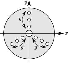
Figure 2. $S_{3g+2}$ embedded in the $xy$-plane

$S_{3g+2}\times[-1,1]$ also admits a symmetry of order 3 by rotating $S_{3g+2}$ about the origin of the $xy$-plane and fixing the $[-1,1]$ factor. These two symmetries generate an action of the dihedral group of order 6 on $S_{3g+2}\times[-1,1]$. It is easy to see that the quotient is a ball. On the other hand, the quotient of $S_{3g+2}\times[-1,1]$ by the order two symmetry is $V_{g}$. This induces the map $f:V_{g}\to B$; note that this is a cover, branched along a trivial tangle with $g+2$ arcs (thus the branch set of the map $M\to S^{3}$ described above is a $g+2$ bridge link, and the braiding is determined by $\bar{f}$). This is Hilden’s construction, see Figure 3, where the branch set of $V_{g}\to B$ is indicated by dashed lines (in $B$).

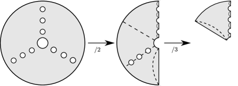
Figure 3. Hilden’s covers

A Heegaard splitting for the manifold with boundary $X$ is a decomposition of $X$ into two compression bodies; we assume the reader is familiar with the basic definitions (see, for example, [5]). We use the notation $V_{g,n}$ for a compression body with $\partial_{+}V_{g,n}$ a genus $g$ surface and $\partial_{-}V_{g,n}$ a collection of $n$ tori (so $0\leq n\leq g$). Since $\partial X$ consists of $n$ tori, any Heegaard splitting of $X$ consists of two compression bodies of the form $V_{g,n_{1}}$ and $V_{g,n_{2}}$, for some $g,n_{1},n_{2}$ with $n_{1}+n_{2}=n$. We use the notation $V_{g,n_{i}}^{*}$ for the manifold obtained by removing $n_{i}$ disjoint open balls from the interior of $V_{g,n_{i}}$. We use the notation $X^{*}$ for the manifold obtained by removing $n$ disjoint open balls from the interior of $X$. Finally, we use the notation $B^{*}_{n_{i}}$ for the manifold obtained by removing $n_{i}$ disjoint open balls from the interior of $B$.

Since compression bodies do not admit simple 3-fold branched covers of the type we need, we work with $V_{g,n_{i}}^{*}$, see Figure 4.

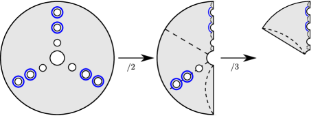
Figure 4. Hilden’s covers modified

Figure 4 is very similar to Figure 3, but has a few “decoration” added in blue. The circles added to $S_{3g+2}\times[-1,1]$ are embedded in $S_{3g+2}\times\{0\}$. There are exactly $3n_{i}$ such circles. Clearly, they are invariant under the dihedral group action, and their images in $V_{g}$ and $B$ are shown. By removing an appropriate neighborhood of these circles and their images, we get a simple 3-fold cover from $V_{g,n_{i}}^{*}$ to $B_{n_{i}}^{*}$.

Applying Hilden’s theorem to the gluing map $f:\partial_{+}V_{g,n_{1}}\to\partial_{+}V_{g,n_{2}}$, we obtained a map $\bar{f}:\partial B_{n_{1}}\to\partial B_{n_{2}}$. Clearly, downstairs we see the manifold obtained by removing $n_{1}+n_{2}=n$ open balls from $S^{3}$; we denote it by $S^{3,*}$.

Note that the branch set is a tangle (that is, a 1-manifold properly embedded in $S^{3,*}$) that intersects every sphere boundary component in exactly 4 points; we denote this branch set by $T$. Moreover, the preimage of each component of $\partial S^{3,*}$ consists of exactly two components: a torus that double covers it, and a sphere that projects to it homeomorphically. The map from the torus in $\partial X^{*}$ to the sphere in $S^{3,*}$ is the quotient under the well known hyperelliptic involution.

Hilden’s construction, as adopted to our scenario, is the key to everything we do below. We sum up its main properties here:

Proposition 6.1.

Let $X$ be a compact, orientable manifold with $\partial X$ consisting of $n$ tori. Let $X^{*}$ be the manifold obtained by removing $n$ open balls from the interior of $X$. Let $S^{3,*}$ be the manifold obtained by removing $n$ open balls from $S^{3}$.

Then there exists a simple 3-fold cover $p:X^{*}\to S^{3,*}$. The branch set is a compact 1-manifold, denoted $T$, that intersects every boundary component of $S^{3,*}$ in exactly four points.

The preimage of each component $S$ of $\partial S^{3,*}$ consists of one torus component of $\partial X$ that double covers $S$ via a hyperelliptic involution, and one sphere component of $\partial X^{*}\setminus\partial X$ that maps to $S$ homeomorphicaly.

Recall that in Theorem 1.6, $X$ came equipped with a choice of meridian and longitude on each boundary component. $S^{3,*}$ is naturally a subset of $S^{3}$. We isotope $S^{3,*}$ in $S^{3}$ so that, after projecting it into the plane, the following conditions hold:

1. The balls removed from $S^{3}$ are denoted $\bar{B}_{i}$ ($i=1\dots,n$). The projection of each $\bar{B}_{i}$ is a round disk; these disks are denoted $B_{i}$, see Figure 5.

   

   Figure 5. $T$ in a neiborhood of $B_{i}$

2. $T$ intersects each $B_{i}$ in exactly four points. Each of these point is an endpoint of a strand of $T$. The four point are the intersection of the lines of slopes $\pm 1$ through the center of the disk with its boundary, and are labeled (in cyclic order) NE, SE, SW, and NW.

3. We twist the boundary components of $S^{3,*}$ so that, in addition, the meridian and longitude of the corresponding boundary component of $\partial X$ map to a horizontal and vertical circles, respectively; thses curves (slightly rounded) are labeled $\mu$ and $\lambda$ in Figure 5.

Let $T_{i}\subset\partial X$ be the torus that projects to $\partial\bar{B}_{i}$. Recall that by Dehn filling $T_{i}$ we mean attaching a solid torus $V$ to $T_{i}$. $V$ is foliated by concentric tori, with one singular leaf (the core circle). To understand how the hyperelliptic involution extends from $\partial V=T_{i}$ into $V$ we construct the following explicit model of the hyperelliptic involution: let $T_{i}$ be the image of $\mathbb{R}^{2}$ under the action of $\mathbb{Z}^{2}$ given by $(x,y)\mapsto(x+n,y+m)$. Then the hyperelliptic involution is given by rotation by $\pi$ about $(0,0)$. The four fixed points on $T_{i}$ are the images of $(0,0)$, $(1/2,0)$ (rotate and translate by $(x+1,y)$), $(0,1/2)$ (rotate and translate by $(x,y+1)$), and $(1/2,1/2)$ (rotate and translate by $(x+1,y+1)$). Given any slope $p/q$ (with $p$ and $q$ relatively prime), it is clear that the foliation of $\mathbb{R}^{2}$ by straight lines of slope $p/q$ is invariant under the rotation by $\pi$ about $(0,0)$. The line through $(0,0)$ goes through $(p/2,q/2)$, which is the image of one of the other three fixed points, as not both $p$ and $q$ are even. Similarly for the lines through $(1/2,0)$, $(0,1/2)$, $(1/2,1/2)$; these lines project to two circles on the torus, with exactly two fixed points on each circle. By considering the images of the foliation of $\mathbb{R}^{2}$ by lines of slope $p/q$, we obtain a foliation of $\partial V$ by circles (each representing the slope $p/q$). In the foliation of $V$ by concentric tori, each torus admits such a foliation, and the length of the leaves limit on $0$ as we approach the singular leaf. At the limit, we see that the involution on the non-singular leaves induces an involution of the singular leaf whose image is an arc. Thus the hyperelliptic involution of $T_{i}$ extends to an involution on $V$, whose image is foliated by spheres, with one singular leaf that is an arc. The image of $V$ is a ball, and the branch set is a rational tangle of slope $p/q$; for more about rational tangles and their double covers see, for example, [22]. We denote this rational tangle by $R_{i}$.

Notation 6.2.

We assume the rational tangles we study have been isotoped to be alternating (it is well known that this can be achieved). Two rational tangles are considered equivalent if the following two conditions hold:

1. The over/under information of the strands of the rational tangles coming in from the NE are the same. Since the rational tangle is alternating, this implies that the over/under information from the other corners is the same as well.

2. The strands of the rational tangles that start at NE end at the same point (SE, SW, or NW).

Note that the crossing information is ill-defined for the two tangles $1/0$ and $0/1$, as they have no crossings. We arbitrarily choose an equivalent class for each of these tangle, so that the second condition is fulfilled. We obtain $6^{n}$ possible equivalence classes (recall that $n={|\partial X|}$).

Given slopes on $T_{1},\dots,T_{n}$, we get rational tangles $R_{1},\dots,R_{n}$, as described above. In each $\bar{B}_{i}$ we place a rational tangle, denoted $\widehat{R}_{i}$, so that $\widehat{R}_{i}\in\{\pm 1,\pm 2,\pm 1/2\}$, representing the same equivalence class as $R_{i}$. We assume that their projections into $B_{i}$ are as in Figure 7. We thus obtain a link, denoted $\widehat{T}$, and a diagram for $\widehat{T}$, denoted $\widehat{D}$. Since $\widehat{T}$ and $\widehat{D}$ only depend on the equivalence classes of the slopes, when considering all possible slopes, we obtain finitely many links and diagrams (specifically, $6^{n}$).

In order to obtain hyperbolic branch set, we will, eventually, apply Mensaco [15] as explained in Subsection 2.4. To that end we will need to make the branch set alternating. As we shall see below, we do this using a $1\to-2$ and $-2\to 1$ Montesinos moves; these moves can be used to make the link alternating in a way that is very similar to crossing changes. Below we will show that we can apply Montesinos moves to $T$, however, we may not apply these moves to the rational tangles inside $B_{i}$. This causes the following trouble: let $\alpha\subset T$ be an interval connecting two punctures, say $\partial\bar{B}_{i}$ and $\partial\bar{B}_{i^{\prime}}$ (possibly, $i=i^{\prime}$). Assume that the last crossing of $R_{i}$ before $\alpha$ is an over crossing, and that the number of crossings along $\alpha$ is even. Then if we make $T$ alternate, the last crossing along $\alpha$ will be an overcrossing. This means that the first crossing of $R_{i^{\prime}}$ after $\alpha$ must be an undercrossing. This may or may not be the case, and we have no control over it.

In order to encode this, we consider the following graph $\Gamma$: $\Gamma$ has $n$ vertices, and they correspond to $B_{1},\dots,B_{n}$. The edges of $\Gamma$ correspond to intervals of $T$ that connect $B_{i}$ to $B_{i^{\prime}}$ (again, $i$ and $i^{\prime}$ may not be distinct). Inspired by the discussion above, we assign signs to the edges of $\Gamma$ as follows (in essence, good edges get a $+$ and bad edges get a $-$):

1. Let $I\subset T$ be an interval connecting $B_{i}$ to $B_{i^{\prime}}$ (possibly $i=i^{\prime}$) so that the last crossing before $I$ and the first crossing after $I$ are the same (that is, both overscrossings or are both undercrossings), and the number of crossings along $I$ is odd. Then the corresponding edge get the sign $+$.

2. Let $I\subset T$ be an interval connecting $B_{i}$ to $B_{i^{\prime}}$ (possibly $i=i^{\prime}$) so that the last crossing before $I$ and the first crossing after $I$ are the opposite (that is, one is an overcrossing and one an undercrossing), and the number of crossings along $I$ is even. Then the corresponding edge get the sign $+$.

3. All other edges get the sign $-$.

If $\Gamma$ is connected, we pick a spanning tree $\widehat{\Gamma}$ for $\Gamma$. That is, $\widehat{\Gamma}$ is a tree obtained from $\Gamma$ by removing edges, so that every vertex of $\Gamma$ is adjacent to some edge of $\widehat{\Gamma}$. In general, we take $\widehat{\Gamma}$ to be a maximal forest in $\Gamma$. A forrest is a collection of trees, or a graph without cycles. A maximal forest in $\Gamma$ is a graph obtained from $\Gamma$ by removing a minimal (with respect to inclusion) set of edges so that a forrest is obtained; equivalently, it is the union of maximal trees for the connected components of $\Gamma$. Clearly a maximal forest $\widehat{\Gamma}$ has the following two properties: first, $\widehat{\Gamma}$ contains no cycles. Second, any edge from $\Gamma$ that we add to $\widehat{\Gamma}$ closes a cycle.

Lemma 6.3.

There is a sign assignment to the vertices of $\widehat{\Gamma}$, so that an edge of $\widehat{\Gamma}$ has a plus sign if and only if the vertices it connects have the same sign.

Proof of Lemma 6.3.

We induct on the number of edges in $\widehat{\Gamma}$. If there are no edges there is nothing to prove.

Assume there are edges. In that case at least one component of $\widehat{\Gamma}$ is a tree with more that one vertex. Such a tree must have a leaf, say $v$. Remove $v$ and $e$, the unique edge of $\widehat{\Gamma}$ connected to $v$. By induction, there is a sign assignment for the remaining vertices fulfilling the conditions of the lemma. We now add $v$ and $e$. Clearly, we can give $v$ a sign so that the condition of the lemma holds for $e$. The lemma follows. ∎

We now isotope $\widehat{T}$ and accordingly modify $\widehat{D}$ as shown in Figure 6

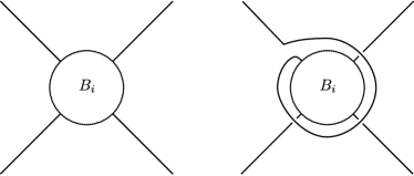
Figure 6. Modifying $\widehat{D}$ near $B_{i}$ (negative sign)

at each puncture that corresponds to a vertex with a minus sign. Since this changes the number of crossings on some of strands of $\Gamma$, we recalculate the signs on the corresponding edges. Note that the isotopy above adds one or three crossing to every strand of $T$ that corresponds to an edge of $\widehat{\Gamma}$ with sign $-$, and zero, two, four, or six crossings to every strand of $T$ that corresponds to an edge with sign $+$. We easily conclude that every edge of $\widehat{\Gamma}$ has sign $+$. Moreover:

Lemma 6.4.

Every edge of $\Gamma$ has sign $+$.

Proof.

The proof is very similar to the proof that every link projection can be made into an alternating link projection via crossing change and is left for the reader, with the following hint: suppose there exists an edge, say $e$, whose sign is $-$. Since we used a maximal forest, there is a cycle in $\Gamma$ (say $e_{1},\dots,e_{k}$) so that $e_{1}=e$ and $e_{i}$ belongs to the maximal forest for $i>1$; in particular, exactly one edge of the cycle has sign $-$. Use this cycle to produce a closed curve (not necessarily simple) in $S^{2}$ that intersects he link $\widehat{T}$ transversely an odd number of times. This is absurd, in light of the Jordan Curve Theorem. ∎

Next we prove that $X^{*}$ can be obtained as a 3-fold cover of $S^{3,*}$ with a particularly nice branch set. We begin with $T$, $\widehat{T}$, and $\widehat{D}$ described above; their properties are summed up in Condition (1) of Lemma 6.5 below. For parts of this argument cf. Blair [3]. Recall Definitions 2.5 for standard terms in knot theory.

Lemma 6.5.

There exists a link $\widehat{T}$ in $S^{3}$, with projection into $S^{2}$ denoted $\widehat{D}$, so that $X^{*}$ is a simple, $3$-fold cover of $S^{3}\setminus\cup_{i=1}^{n}\mbox{\rm int}(\bar{B}_{i})$ branched along the tangle $T=\widehat{T}\cap(S^{3}\setminus\cup_{i}\mbox{\rm int}(B_{i}))$ and the following conditions hold:

1. $\widehat{T}\cap\bar{B}_{i}=\widehat{R}_{i}$ (recall that $\widehat{R}_{i}$ projects into $B_{i}$ as shown in Figure 7),

   

   Figure 7. $\hat{R}_{i}$, the representatives for equivalence classes

   the projection of $\mbox{int}(T\setminus\widehat{T})$ is disjoint from $\cup_{i=1}^{n}B_{i}$, and the meridian and longitude of $T_{i}\subset\partial X$ project to horizontal and vertical circles about $B_{i}$ (respectively, recall Figure 5).

2. $\widehat{D}$ is not a split diagram.

3. Every simple closed curve in $S^{2}\setminus\cup B_{i}$ that intersects $\widehat{D}$ transversely in two simple point bounds a disk that intersects $\widehat{D}$ in a single arc with no crossing.

4. Let $\alpha\subset S^{2}$ be an arc with one endpoint on $B_{i^{\prime}}$ and the other on $B_{i^{\prime\prime}}$ (for $i^{\prime},\ i^{\prime\prime}=1,\dots,n$, possibly $i^{\prime}=i^{\prime\prime}$), and $\mbox{\rm int}(\alpha)\cap(\cup_{i}B_{i})=\emptyset$. Then one of the following conditions holds:

   1. $i^{\prime}=i^{\prime\prime}$, and $\alpha$ cobounds a disk with $\partial B_{i}$ with no crossings.

   2. $|\mbox{int}(\alpha)\cap\widehat{D}|>2$.

5. In the three coloring of $\widehat{D}\cap(S^{2}\setminus\cup_{i=1}^{n}B_{i})$ induced by the cover $X^{*}\to S^{3,*}$, every crossing is three colored.

6. $\widehat{D}$ is alternating.

7. $\widehat{T}$ is a knot.

Remark 6.6.

To obtain conditions (1)–(5) we modify $\widehat{T}$ via isotopy; except for the move shown in Figure 9, the projection of the support of this isotopy is disjoint from $\cup_{i=1}^{n}B_{i}$. Note that in the move shown in Figure 9 each edge gets and even number of crossings added. Hence the signs of the edges of $\Gamma$ do not change, and Lemma 6.4 still holds after we obtain Conditions (1)–(5). (We use this lemma to obtain Condition (6), and never need it again after that.)

Proof.

Condition (1). Condition (1) already holds. We note that none of the moves applied in the proof of this lemma changes this. We will not refer to Condition (1) explicitly.

Condition (2). $\widehat{D}$ is diagrammatically split if and only if it is disconnected. Suppose $\widehat{D}$ is disconnected, and let $K_{j}$ and $K_{j^{\prime}}$ be components of $\widehat{T}$ that project to distinct components of $\widehat{D}$. Let $\alpha\subset S^{2}\setminus\cup_{i=1}^{n}B_{i}$ be an embedded arc with one endpoint on $K_{j}$ and the other on $K_{j^{\prime}}$ (note that $K_{j},\ K_{j^{\prime}}\not\subset\cup_{i=1}^{n}B_{i}$, hence $\alpha$ exists; $\alpha$ may intersect $\widehat{D}$ in its interior). We perform an isotopy along $\alpha$, as shown in Figure 8.

Figure 8. Isotopy along $\alpha$

After that $K_{j}$ crosses $K_{j^{\prime}}$ outside $\cup_{i=1}^{n}B_{i}$; clearly, this reduces the number of components of $\widehat{D}$. Repeating this process if necessary, Condition (2) is obtained.

Condition (3). For each $B_{i}$, let $N(B_{i})$ be a normal neighborhood of $B_{i}$ so that $\widehat{D}\cap N(B_{i})$ consists of the tangle in $B_{i}$ and four short segments as in the left hand side of Figure 9. We assume further that for $i\neq j$, $N(B_{i})\cap N(B_{j})=\emptyset$.

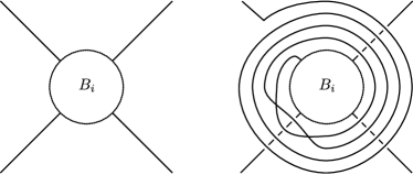
Figure 9. Isolating $B_{i}$

Inside each $N(B_{i})$ perform the isotopy shown in Figure 9.

Next we count the number of simple closed curves in $S^{2}\setminus\cup_{i}B_{i}$ that intersect $\widehat{D}$ in two points and do not bound a disk $\Delta$ with $\widehat{D}\cap\Delta$ is a single arc with no crossings. These curves are counted up to “diagrammatic isotopy”, that is, an isotopy via curves that are transverse to $\widehat{D}$ at all time and in particular are disjoint from the crossings.

Let $C_{1},\dots,C_{k}$ be the closures of the components of $S^{2}\setminus(\widehat{D}\cup(\cup_{i}B_{i}))$. Let $\gamma,\gamma^{\prime}\subset S^{2}\setminus\cup_{i}B_{i}$ be two simple closed curves that intersects $\widehat{D}$ transversely in two simple points. Then $\widehat{D}$ cuts $\gamma$ into 2 arcs, say one in the region $C_{j}$ and one in $C_{j^{\prime}}$. Note that if $j=j^{\prime}$, then $C_{j}$ is adjacent to itself, and in particular there is a simple closed curve in $S^{2}$ that intersects $\widehat{D}$ transversely in one point, which is absurd. Condition (2) (connectivity of $\widehat{D}$) is equivalent to all regions being disks, and hence implies that $\gamma$ and $\gamma^{\prime}$ are diagrammatically isotopic if and only if both curves traverse the same regions $C_{j}$ and $C_{j^{\prime}}$, and $\gamma\cap\partial C_{j}$ is contained in the same segments of $C_{j}\cap C_{j^{\prime}}$ as $\gamma^{\prime}\cap\partial C_{j^{\prime}}$. (See Figure 10;

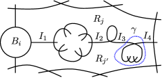
Figure 10. Segments

here a segment means an interval $I\subset S^{2}\setminus\cup_{i}\mbox{int}(B_{i})$, so that $I\subset C_{j}\cap C_{j^{\prime}}$, $\partial I$ are crossings or lie on $\partial B_{i}$ for some $i$, and $I$ contains no crossings in its interior.) For any pair of regions $C_{j}$ and $C_{j^{\prime}}$, let $n_{j,j^{\prime}}$ be the number of segments in $C_{j}\cap C_{j^{\prime}}$ (for example, in Figure 10, $n_{j,j^{\prime}}=4$). Then we see that the number of simple closed curves that intersect $\widehat{D}$ in two simple points, traverse $C_{j}$ and $C_{j^{\prime}}$, and do not bound a disk containing a single arcs of $\widehat{D}$ (counted up to diagrammatic isotopy) is ${n_{j,j^{\prime}}}\choose{2}$, where ${0}\choose{2}$ and ${1}\choose{2}$ are naturally understood to be 0. Hence the total number of such curves (counted up to diagrammatic isotopy) is

(2) $$\sum_{1\leq j<j^{\prime}\leq k}{n_{j,j^{\prime}}\choose 2}.$$

Now assume that condition (3) does not hold; then there exist regions $C_{j}$ and $C_{j^{\prime}}$ with $n_{j,j^{\prime}}\geq 2$. Let $I$ be an interval of $C_{j}\cap C_{j^{\prime}}$. Since we isolated $B_{i}$ (for all $i$) as shown in Figure 9, the endpoints of $I$ cannot lie on $\partial B_{i}$ and must therefore both be crossings. The move shown in Figure 11

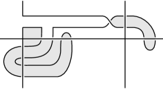
Figure 11. Isotopy to reduce $C_{i,i^{\prime}}$

reduces $n_{j,j^{\prime}}$ by one. This move introduces several new regions, and those are shaded in Figure 11. Inspecting Figure 11, we see that for any pair of regions $C_{j}$, $C_{j^{\prime}}$ that existed prior to the move, $n_{j,j^{\prime}}$ does not increase, and for any pair of regions $C_{j}$, $C_{j^{\prime}}$ with at least one new region, $n_{j,j^{\prime}}$ is 1 or 0. Hence the sum in Equation (2) is reduced, and repeated application of this move yields a diagram $\widehat{D}$ for a link $\widehat{T}$ for which Condition (3) holds; by construction, Condition (2) still holds.

Condition (4). Condition (4) holds thanks to the isotopy performed in the previous step and shown in Figure 9.

Condition (5). Since $\widehat{D}$ is the branch set of the simple 3-fold cover $X^{*}\to S^{3,*}$ it inherits a 3-coloring as explained in Subsection 2.1, where the colors are transpositions in $S_{3}$. Since $X^{*}$ is connected, at least two colors appear in the coloring of $T$ (recall Lemma 2.4; that lemma was stated for covers of $S^{3}$ but it is easy to see that it holds for covers of $S^{3,*}$ as well).

Assume there exists a one colored crossing of $\widehat{D}$ outside $\cup_{i=1}^{n}B_{i}$, say $c$, and let $p$ be a point on a strand of $\widehat{D}$ that is of a different color than $c$, and so that $p\not\in\cup_{i=1}^{n}B_{i}$. Let $\alpha$ be an arc connecting $p$ and $c$ so that $\alpha\cap(\cup_{i=1}^{n}B_{i})=\emptyset$. If $\mbox{int}(\alpha)$ intersects a strand of $\widehat{D}$ whose color is different than the color of $c$, we cut $\alpha$ short at that intersection. Thus we may assume that any point of $\mbox{int}(\alpha)\cap\widehat{D}$ has the same color as $c$. We apply the following move (often used by Hilden, Montesinos and others), see Figure 12.

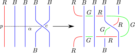
Figure 12. Making the crossings 3-colored

This move reduces the number of one colored corssings outside $\cup_{i}B_{i}$, and hence repeating this move gives Condition (5).

We now verify that Conditions (2)–(4) still hold. Inspecting Figure 12, we see that Condition (2), which is equivalent to connectivity of $\widehat{D}$, clearly holds. A simple closed curves that intersects $\widehat{D}$ twice after this moves, intersects it at most twice before the move. By considering these curves and Figure 12 we conclude that Condition (3) holds as well (in checking this, note that $\mbox{int}\alpha\cap\widehat{D}$ maybe empty; to rule out one case, you need to use the coloring: a red arc cannot be connected to a blue arc without a crossing). For each $i$, the preimage of $\partial\bar{B}_{i}$ is disconnected; hence the four segments of $\widehat{D}$ on the left side of Figure 9 are all the same color. Since $\widehat{D}$ is connected and has more than one color, is must have a three colored crossing, which cannot be contained in $N(B_{i})$ for any $i$. We can take the point $p$ in the construction above to be a point near that three colored crossing, and in particular, we may assume that $p\not\in N(B_{i})$ for any $i$. Therefore this move effects $\widehat{D}\cap N(B_{i})$ by adding arcs that traverse $N(B_{i})$ without interscting $B_{i}$ itself, but not changing any of the existing diagram in the right hand side of Figure 9. Therefore Condition (4) holds.

Condition (6). Note that the tangles $\widehat{R}_{i}$ are alternating ($i=1,\dots,n$). It is well known that any link projection can be made into an alternating projection by reversing some of its crossings. We mark the crossings of $\widehat{D}$ by $\pm$, marking a crossing $+$ if we do not need to reverse it and $-$ otherwise. By reversing all the signs if necessary, we may assume that the signs in $B_{1}$ are $+$. Since the signs of all the edges of $\Gamma$ are $+$ (Lemma 6.4 and Remark 6.6), the signs in every $B_{i}$ are all $+$. Thus all the crossings that are marked $-$ are outside $\cup_{i=1}^{n}B_{i}$, and hence three colored. We change each of this crossing using the Montesinos move $+1\mapsto-2$ or $-1\mapsto+2$, as in the top row of Figure 1, noting that this does not change the double cover. It is clear that now $\widehat{D}$ is an alternating diagram fulfilling Conditions (1)–(6).

Condition (7). Assume $T$ is a link. If there is a crossing outside $\cup_{i}B_{i}$ that corresponds to two distinct components of $T$, we perform a $+1\mapsto+4$ or $-1\mapsto-4$ Montesinos move; this reduces the number of components of $T$. Assume there is no such crossing, and let $\alpha$ be an arc connecting strands (say $s_{1}$ and $s_{2}$) that correspond to two distinct components of $T$. Since no $B_{i}$ contains a closed component, we may assume $\alpha\cap(\cup_{i}B_{i})=\emptyset$; furthermore, by truncating $\alpha$ if necessary, we may assume that $\mbox{int}\alpha\cap\widehat{D}=\emptyset$. By Condition (4) at least one endpoint of $s_{2}$ is a crossing outside $\cup_{i}B_{i}$, say $c$. If $s_{1}$ and $s_{2}$ have the same color, we replace $\alpha$ with an arc that connects $s_{1}$ with a strand adjacent to $s_{2}$ at $c$. By Condition (5) $c$ is three colored, and by assumption, both its strands correspond to the same component of $T$. Thus we obtain an arc that connects distinct components and has endpoints of different colors. Finally, we assume without loss of generality that the crossing information at $s_{1}$ is as shown in Figure 13. Since $\widehat{D}$ is connected and alternating, considering the face containing $\alpha$, we conclude that the crossing information on $s_{2}$ is as shown in that figure. We change $\widehat{D}$ using a $0\mapsto\pm 3$ Montasinos move (as shown in the bottom of Figure 1), obtaining a diagram fulfilling Conditions (1)–(6) that corresponds to a link with fewer components, see Figure 13.

Figure 13. Making the brach set into a knot

Iterating this process, we obtain a knot, completing the proof of of Lemma 6.5 ∎

We are now ready to complete the proof of Theorem 1.6. Fix $X$ as in the statement of the theorem and pick a slope on each components of $\partial X$, say $p_{i}/q_{i}$ on the torus $T_{i}\subset\partial X$; note that we are using the meridian-longitudes to express the slpes as rational numbers (possibly, $1/0$). Construct a 3-fold, simple cover $X^{*}\to S^{3,*}$ as in Lamme 6.5 that corresponds to the appropriate equivalence classes of the slopes (recall Notation 6.2). For convenience we work with $\widehat{D}$, the digram of $\widehat{T}$.

We now change the diagram $\widehat{D}$ by replacing the rational tangle $\widehat{R}_{i}$ in $B_{i}$ (that represents the equivalence class of $p_{i}/q_{i}$) with the rational tangle $R_{i}$ (that realizes the slope $p_{i}/q_{i}$), $i=1,\dots,n$. By construction the four strands of $\widehat{D}$ that connect to $B_{i}$ are single colored, and we color the $R_{i}$ by the same color. Thus we obtain a diagram of a three colored link denoted $K$.

We claim that $K$ has the following properties:

1. $K$ is a knot.

2. $K$ admits an alternating projection.

3. This projection is non-split.

4. This projection is strongly prime.

We prove each claim in order:

1. Since the tangles $\widehat{R}_{i}$ and $R_{i}$ are equivalent they connect the same points on $\partial B_{i}$ (Notation 6.2). By Lemma 6.5 (7), $\widehat{T}$ is a knot. Hence $K$, which is obtained from $\widehat{T}$ by replacing $\widehat{R}_{i}$ by $R_{i}$, is a knot as well.

2. By Lemma 6.5 (6), $\widehat{D}$ is alternating. By the definition of the equivalence classes of rational tangles, $K$ (which is obtained by replacing $\widehat{R}_{i}$ by $R_{i}$) admits an alternating projection.

3. Let $\gamma\subset S^{2}$ be a simple closed curve disjoint from the diagram for $K$. If $\gamma$ is diagrammatically isotopic (that is, an isotopy through curves that are transverse to the diagram at all times) to a curve that is disjoint from $\cup_{i}B_{i}$ then by Lemma 6.5 (2) $\gamma$ bounds a disk disjoint from $\widehat{D}$; this disk is also disjoint from the diagram of $K$. If $\gamma$ is diagrammatically isotopic into $B_{i}$, then $\gamma$ bounds a disk disjoint from the diagram for $K$ since rational tangles are prime. Finally, if $\gamma$ is not isotopic into or out of $\cup_{i}B_{i}$, we violate Condition (4b) of Lemma 6.5. Hence the diagram for $K$ is non-split.

4. This is very similar to (3) and is left to the reader.

By Menasco and Thurston (see Corollary 2.8), $K$ is hyperbolic.

Next we note that the 3-coloring of $K$ defines a $3$-fold cover of $S^{3}$; by construction, the cover of $S^{3,*}$ is $X^{*}$. The cover of each rational tangle is disconnected and consists of a solid torus attached to $T_{i}\subset\partial X$ with slope $p_{i}/q_{i}$, and a ball attached to a component of $\partial X^{*}\setminus\partial X$. Thus we obtain $X(p_{1}/q_{1},\dots,p_{n}/q_{n})$ as a simple $3$-fold cover of $S^{3}$ branched over $K$.

We now isotope each rational tangle $R_{i}$ to realize its depth, that is, realizing the twist number of each rational tangle (recall Subsection 2.5). The twist number of $R_{i}$ is exactly $\mbox{\rm depth}(p_{i}/q_{i})$. The tangle $T$ (which is the projection of $K$ outside $\cup_{i}B_{i}$) has a fixed number of twist regions, say $t$. Hence the total number of twist regions is $t+\sum_{i=1}^{n}\mbox{\rm depth}(p_{i}/q_{i})=t+\mbox{\rm depth}(\alpha)$ (where $\alpha=(\alpha_{1},\dots,\alpha_{n})$ denotes the multislope on $\partial X$, as in Section 1). This gives an upper bound for the twist number for $K$:

$$t(K)\leq t+\mbox{\rm depth}(\alpha).$$

Lackenby [13] (recall Subsection 2.5) showed that there exists a constant $c$ so that:

$$\mbox{\rm Vol}(S^{3}\setminus K)\leq ct(K).$$

Hence we get:

$$\mbox{\rm KnotVol}_{s,{3}}(X(\alpha_{1},\dots,\alpha_{n})) \leq 3\mbox{\rm Vol}(S^{3}\setminus K)$$

$$\leq 3ct(K)$$

$$\leq 3ct+3c(\mbox{\rm depth}(\alpha)).$$

By setting $A=3c$ and $B=3ct$, we obtain constants fulfilling the requirements of Theorem 1.6 that are valid for any multislope $\alpha^{\prime}=(\alpha_{1}^{\prime},\dots,\alpha_{n}^{\prime})$, with $\alpha_{i}^{\prime}$ in the same equivalence class as $\alpha_{i}$. As there are only finitely many (specifically, $6^{n}$) equivalence classes, taking the maximal constants $A$ and $B$ for these classes completes the proof of the theorem.

References

- [1] James W. Alexander. Note on Riemann spaces. Bull. Amer. Math. Soc., 26(8):370–372, 1920.
- [2] Riccardo Benedetti and Carlo Petronio. Lectures on hyperbolic geometry. Universitext. Springer-Verlag, Berlin, 1992.
- [3] Ryan C. Blair. Alternating augmentations of links. J. Knot Theory Ramifications, 18(1):67–73, 2009.
- [4] Chun Cao and G. Robert Meyerhoff. The orientable cusped hyperbolic -manifolds of minimum volume. Invent. Math., 146(3):451–478, 2001.
- [5] A. J. Casson and C. McA. Gordon. Reducing Heegaard splittings. Topology Appl., 27(3):275–283, 1987.
- [6] Mark E. Feighn. Branched covers according to J. W. Alexander. Collect. Math., 37(1):55–60, 1986.
- [7] C. McA. Gordon and J. Luecke. Knots are determined by their complements. J. Amer. Math. Soc., 2(2):371–415, 1989.
- [8] Hugh M. Hilden. Every closed orientable -manifold is a -fold branched covering space of . Bull. Amer. Math. Soc., 80:1243–1244, 1974.
- [9] Hugh M. Hilden, María Teresa Lozano, and José María Montesinos. The Whitehead link, the Borromean rings and the knot are universal. Collect. Math., 34(1):19–28, 1983.
- [10] Hugh M. Hilden, María Teresa Lozano, and José María Montesinos. On knots that are universal. Topology, 24(4):499–504, 1985.
- [11] Tsuyoshi Kobayashi and Yo’av Rieck. A linear bound on the tetrahedral number of manifolds of bounded volume (after Jørgensen and Thurston). Contemporary Mathematics, 560:27–42, 2011.
- [12] Sadayoshi Kojima. Isometry transformations of hyperbolic -manifolds. Topology Appl., 29(3):297–307, 1988.
- [13] Marc Lackenby. The volume of hyperbolic alternating link complements. Proc. London Math. Soc. (3), 88(1):204–224, 2004. With an appendix by Ian Agol and Dylan Thurston.
- [14] W. B. Raymond Lickorish. An introduction to knot theory, volume 175 of Graduate Texts in Mathematics. Springer-Verlag, New York, 1997.
- [15] W. Menasco. Closed incompressible surfaces in alternating knot and link complements. Topology, 23(1):37–44, 1984.
- [16] Edwin E. Moise. Affine structures in -manifolds. V. The triangulation theorem and Hauptvermutung. Ann. of Math. (2), 56:96–114, 1952.
- [17] José M. Montesinos. A representation of closed orientable -manifolds as -fold branched coverings of . Bull. Amer. Math. Soc., 80:845–846, 1974.
- [18] Kimihiko Motegi and Yo’av Rieck. Short geodesic after dehn filling. In preparation.
- [19] Robert Myers. Simple knots in compact, orientable -manifolds. Trans. Amer. Math. Soc., 273(1):75–91, 1982.
- [20] Walter D. Neumann and Don Zagier. Volumes of hyperbolic three-manifolds. Topology, 24(3):307–332, 1985.
- [21] Jair Remigio-Juárez and Yo’av Rieck. The link volumes of some prism manifolds. Accepted to Algebraic and Geometric Topology, 2012.
- [22] Dale Rolfsen. Knots and links, volume 7 of Mathematics Lecture Series. Publish or Perish Inc., Houston, TX, 1990. Corrected reprint of the 1976 original.
- [23] William P Thurston. The geometry and topology of 3-manifolds. available from msri.org.