Casimir Energy of the Universe and the Dark Energy Problem

Abstract

We regard the Casimir energy of the universe as the main contribution to the cosmological constant. Using 5 dimensional models of the universe, the flat model and the warped one, we calculate Casimir energy. Introducing the new regularization, called sphere lattice regularization, we solve the divergence problem. The regularization utilizes the closed-string configuration. We consider 4 different approaches: 1) restriction of the integral region (Randall-Schwartz), 2) method of 1) using the minimal area surfaces, 3) introducing the weight function, 4) generalized path-integral. We claim the 5 dimensional field theories are quantized properly and all divergences are renormalized. At present, it is explicitly demonstrated in the numerical way, not in the analytical way. The renormalization-group function ($\beta$-function) is explicitly obtained. The renormalization-group flow of the cosmological constant is concretely obtained.

1 Introduction

At present, the energy budget of the universe is not explained theoretically. We do not understand the dark matter and the dark energy. The latter one, which is the present main topic, is regarded as the same problem as the cosmological constant one, which is the long-lasting problem[1, 2]. As for the problem, Polyakov[3, 4] made a notable conjecture that the cosmological constant, just like the QED coupling, flows to a small value in the IR region (screening phenomena). He made another comment[5] that the dark energy, like the black body radiation 150 years ago, hides secrets of fundamental physics. These views about the problem look to be revived in the recent strong trend of the AdS/CFT (holography) approach to the condensed matter physics or to the viscous fluid dynamics(Navier-Stokes equation)[6, 7].

The difficulty of the problem is strongly related to the unsuccessful situation of the quantum gravity. It also has the long research history since Feynman initiated in 1963[8] until the present string or D-brane research. In the microscopic side, the gravitational interaction has, when quantized, serious UV-divergences[9], while , in the macroscopic one, it has serious IR-divergences around the horizon (boundaries)[10, 4].

About 2 years ago (2010 January), Verlinde[11] made a shocking view about the role of the gravitational force. He made a very thoughtful analysis, including some Gedanken-experiments, about the gravitational force and finally reached the conclusion that the gravitational interaction (force) is not fundamental but is emergent (by some still-obscure mechanism). He referred some (not few) past literature about similar stand points such as Jacobson’s[12] and Padmanabhan’s[13]. The analysis demands very delicate treatment of the horizon which is the boundary of the theory. The physical quantities (IR-)diverge at the horizon. It strongly indicates the regularization problem in the near-horizon treatment where Hawking radiation (thermalization) occurs.

The biggest discrepancy, in all physical quantities, between observation and theory appears in the cosmological constant $\lambda$.

$$S=\int d^{4}x\sqrt{-g}\{\frac{1}{16\pi G_{N}}(R-2\lambda)+{\cal L}_{matter}\}\ {\quad,}$$

$$\frac{\lambda_{th}}{\lambda_{obs}}\sim N_{DL}^{~{}2}{\quad,}\quad N_{DL}\equiv M_{pl}R_{cos}\sim 6.\times 10^{60}{\quad,}$$ (1)

where $M_{pl}$ ($\equiv 1/\sqrt{G_{N}}$) and $R_{cos}$ ($\equiv 1/H_{0},H_{0}:$ Hubble constant) are Planck mass and the size of the universe respectively. $N_{DL}$ is an analog of Dirac’s large number[14]. The cause of the theoretical difficulty lies in the two extreme-ends of mysterious branches of physics: the quantum gravity and the cosmology.

Casimir energy is generally the vacuum energy of the free-part of the system dynamics. For the harmonic oscillator, it is the energy of the zero-point oscillation. By definition, it is independent of the coupling. It depends, however, on the boundaries and the system topology. It is caused by the quantum fluctuation. Because we have to deal with serious UV and IR divergences, highly-delicate regularization is required. The well-known one is that for the 4D electromagnetism (free wave theory). The system of two parallely-placed metalic plates separated by the length $l$, has Casimir energy as follows.

$$\mbox{4D Space-time}:\ V_{Cas}(l)=\frac{B_{4}}{l^{3}},\ \ F_{Cas}(l)=-\frac{\partial V}{\partial l}=3\frac{B_{4}}{l^{4}},\ \ B_{4}(\mbox{4-th Bernoulli No})=-\frac{1}{30},$$

$$\mbox{5D Space-time}:\ V_{Cas}(l)=-\frac{3}{32\pi^{2}}\frac{\zeta(5)}{l^{4}},\ \ F_{Cas}(l)=-\frac{\partial V}{\partial l}=-\frac{3}{8\pi^{2}}\frac{\zeta(5)}{l^{5}},\ \ \zeta(5)=1.03693\cdots.$$ (2)

2 Casimir Energy of 5 Dimensional Electromagnetism

For the electromagnetism in the flat 5D space-time ($ds^{2}=\eta_{\mu\nu}dx^{\mu}dx^{\nu}+dy^{2},~{}\eta_{\mu\nu}=\mbox{diag}(-1,1,1,1)$), Casimir energy is given by [15]

$$E_{Cas}(\Lambda,l)={\int_{{\tilde{p}}\leq\Lambda}\frac{d^{4}p}{(2\pi)^{4}}}\int_{0}^{l}dy(F_{f}^{-}({\tilde{p}},y)+4F_{f}^{+}({\tilde{p}},y)){\quad,}$$

$$F_{f}^{\mp}({\tilde{p}},y)=-\int_{\tilde{p}}^{\infty}d{\tilde{k}}\frac{\mp\cosh{\tilde{k}}(2y-l)+\cosh{\tilde{k}}l}{2\sinh({\tilde{k}}l)}{\quad,}$$ (3)

where $\mp$ is the $y$-parity ($y\leftrightarrow-y$), $l$ is the periodicity $y\rightarrow y+2l$, and $\Lambda$ is the momentum cut-off. ${\tilde{p}}$ is the magnitude of the 4D Euclidean momentum $(p_{1},p_{2},p_{3},p_{4}=ip_{0})$. This is consistent with Ref.[16].

As for the warped (AdS₅) geometry, $ds^{2}=(\eta_{\mu\nu}dx^{\mu}dx^{\nu}+dz^{2})/\omega^{2}z^{2}$ ($\omega$: 5D curvature), the corresponding one is given by [17]

$$-E^{\Lambda,\mp}_{Cas}(\omega,T)=\left.{\int\frac{d^{4}p_{E}}{(2\pi)^{4}}}\right|_{{\tilde{p}}\leq\Lambda}\int_{1/\omega}^{1/T}dz~{}F_{w}^{\mp}({\tilde{p}},z),F_{w}^{\mp}({\tilde{p}},z)=\frac{1}{(\omega z)^{3}}\int_{{\tilde{p}}^{2}}^{\infty}\{G_{k}^{\mp}(z,z)\}dk^{2},$$

$$G_{p}^{\mp}(z,z^{\prime})=\mp\frac{\omega^{3}}{2}z^{2}{z^{\prime}}^{2}\frac{\{{\bf I}_{0}(\frac{{\tilde{p}}}{\omega}){\bf K}_{0}({\tilde{p}}z)\mp{\bf K}_{0}(\frac{{\tilde{p}}}{\omega}){\bf I}_{0}({\tilde{p}}z)\}\{{\bf I}_{0}(\frac{{\tilde{p}}}{T}){\bf K}_{0}({\tilde{p}}z^{\prime})\mp{\bf K}_{0}(\frac{{\tilde{p}}}{T}){\bf I}_{0}({\tilde{p}}z^{\prime})\}}{{\bf I}_{0}(\frac{{\tilde{p}}}{T}){\bf K}_{0}(\frac{{\tilde{p}}}{\omega})-{\bf K}_{0}(\frac{{\tilde{p}}}{T}){\bf I}_{0}(\frac{{\tilde{p}}}{\omega})},$$ (4)

where ${\bf I}_{0}$ and ${\bf K}_{0}$ are 0-th modified Bessel functions. For simplicity, we take the bulk particle mass M in such a way that $M^{2}=-4\omega^{2}<0$. $T$ is defined by $T=\omega\exp({-l\omega})$.

3 Behavior of Casimir Energy

The integral region, for the flat case (3), is shown in Fig.2. $\mu$ and $\epsilon$ are the IR cutoff of ${\tilde{p}}$-axis and the UV cutoff of $y$-axis respectively. Fig.2 shows the integrand of (3): ${\tilde{p}}^{3}(F_{f}^{-}+4F_{f}^{+})\equiv{\tilde{p}}^{3}F({\tilde{p}},y)$.

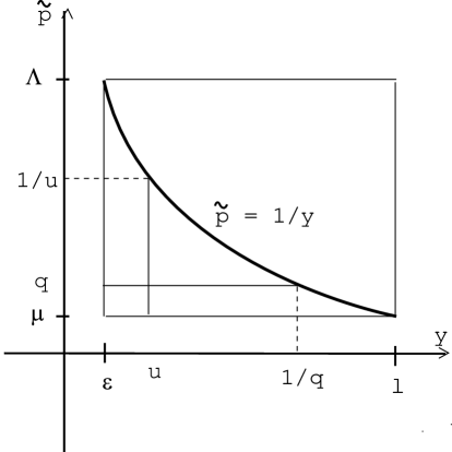
Figure 1: Space of (y,${\tilde{p}}$) for the integration (3). The hyperbolic curve is used in (6).

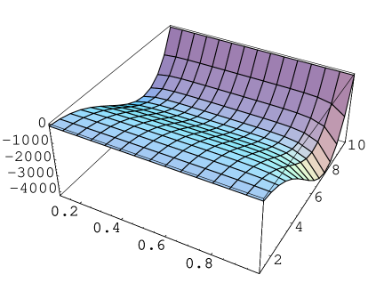
Figure 2: Behaviour of ${\tilde{p}}^{3}F({\tilde{p}},y)$ in (3). $l=1$, $\Lambda=10$, $0.1\leq y<1$, $1\leq{\tilde{p}}\leq 10$ .

In Fig.3 the behavior of the integrand of $F^{-}$ (3) is shown. The (inverse) table shape says the ”Rayleigh-Jeans” dominance because Casimir energy density is proportinal to the cubic power of ${\tilde{p}}$ in the region ${\tilde{p}}\ll\Lambda$.

Figure 3: Behaviour of the integrand of $F^{-}$,(3). $l=1$, $\Lambda=100$, $0\leq y\leq l=1$, $1\leq{\tilde{k}}\leq\Lambda=100$ . The flat plane locates at the height -0.5.

Numerically $E_{Cas}(\Lambda,l)$ is obtained as

$$E_{Cas}(\Lambda,l)=\frac{2\pi^{2}}{(2\pi)^{4}}\left[-0.1249l\Lambda^{5}-(1.41,0.706,0.353)\times 10^{-5}~{}l\Lambda^{5}\ln(l\Lambda)\right]{\quad.}$$ (5)

In Fig.2, the region below the hyperbolic curve is that of Randall-Schwartz(RS)[18]. They claimed the rectangular region should be replaced by this restricted one for the purpose of reducing the divergences.

$$E^{RS}_{Cas}=\frac{2\pi^{2}}{(2\pi)^{4}}\int_{1/l}^{\Lambda}dq\int_{1/\Lambda}^{1/q}dy~{}q^{3}F(q,y)=\frac{2\pi^{2}}{(2\pi)^{4}}[-8.93814\times 10^{-2}~{}\Lambda^{4}]{\quad,}$$ (6)

which shows slightly milder than (5). $\ln(l\Lambda)$-term does not appear.

As for the Warped model, the situation is similar. Fig.5 shows the integral region. The z-axis range is $\omega^{-1}\leq z\leq T^{-1}$. We take IR-regularization-point of ${\tilde{p}}$ as $\mu=\Lambda T/\omega$. In Fig.5 the behavior of the integrand of $E^{-}_{Cas}$ (4) is shown. Fig.6 shows the warped version of Fig.3. $E^{-}_{Cas}$ (4) is numerically obtained as

$$E^{\Lambda,-}_{Cas}(\omega,T)=\frac{2\pi^{2}}{(2\pi)^{4}}\times\left[-0.0250\frac{\Lambda^{5}}{T}\right]{\quad,}$$ (7)

which does not depend on $\omega$ and has no $\ln(\Lambda/T)$ term. When restricted to RS-region, the above value changes to

$$E^{-RS}_{Cas}(\omega,T)=\frac{2\pi^{2}}{(2\pi)^{4}}\int_{\mu}^{\Lambda}dq\int_{1/\omega}^{\Lambda/\omega q}dz~{}q^{3}F^{-}(q,z)$$

$$=\frac{2\pi^{2}}{(2\pi)^{4}}\frac{\Lambda^{5}}{\omega}\left\{-1.58\times 10^{-2}-1.69\times 10^{-4}\ln~{}\frac{\Lambda}{\omega}\right\}{\quad,}$$ (8)

which is independent of T and has the $\ln(\Lambda/\omega)$ term. Divergence behavior is the same as the unrestricted case (7).

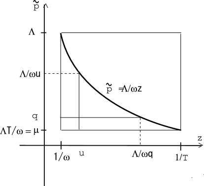
Figure 4: Space of (z,${\tilde{p}}$) for the integration (4). The hyperbolic curve is used in (8).

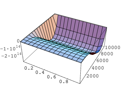
Figure 5: Behaviour of $(-1/2){\tilde{p}}^{3}F^{-}({\tilde{p}},z)$ in (4). $T=1,\omega=10^{4},\Lambda=10^{4}$. $1.0001/\omega\leq z<0.9999/T$, $\Lambda T/\omega\leq{\tilde{p}}\leq\Lambda$.

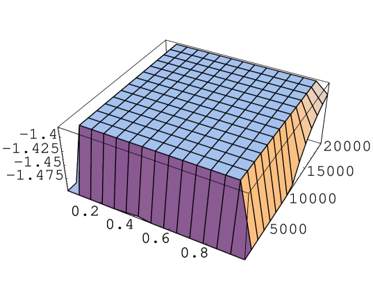
Figure 6: Behavior of $\ln|{\frac{1}{2}}{\cal F}^{-}({\tilde{k}},z)|=\ln|{\tilde{k}}~{}G^{-}_{k}(z,z)/(\omega z)^{3}|$. $\omega=10^{4},T=1,\Lambda=2\times 10^{4}$. $1.0001/\omega\leq z\leq 0.9999/T$. $\Lambda T/\omega\leq{\tilde{k}}\leq\Lambda$. Note $\ln|(1/2)\times(1/2)|\approx-1.39$.

4 Sphere Lattice Regularization

The Randall-Schwartz’s way of restricting the integral region does not sufficiently work to reduce the divergences. In Ref.[19], we proposed a new way of the restriction based on the isotropy property of the system and the minimal area principle. Let us introduce two 4D hyper-surfaces, B_UV and B_IR, in the 5D bulk space-time.

$$\mbox{B}_{UV}\quad:\quad{\tilde{p}}^{-1}=\sqrt{(x^{1})^{2}+(x^{2})^{2}+(x^{3})^{2}+(x^{4})^{2}}=r_{UV}(y){\quad,}\quad\epsilon=\frac{1}{\Lambda}<y<l{\quad,}$$

$$\mbox{B}_{IR}\quad:\quad{\tilde{p}}^{-1}=\sqrt{(x^{1})^{2}+(x^{2})^{2}+(x^{3})^{2}+(x^{4})^{2}}=r_{IR}(y){\quad,}\quad\epsilon=\frac{1}{\Lambda}<y<l{\quad,}$$ (9)

where $x^{a}\ (a=1,2,3,4)$ is Euclidian coordinate. See Fig.8 and Fig.8. The surfaces, in the ”brane” located at $y$, are 3D sphere with the radius $r(y)$. The radius changes along the extra axis $y$. The function form of $r(y)$ is given by the minimal area (of the hyper surface) principle. We integrate the region bounded by B_IR from below and by B_UV from above as shown in Fig.8. Some regularization parameters ($\Lambda,\mu,\Lambda^{\prime},\mu^{\prime},\varepsilon$) are defined there. The renormalization group interpretation is shown in Fig.8. The surface B_UV is stereo-graphically shown in Fig.10. It shows the present regularization utilizes the closed-string configuration. The integral region for the warped case is shown in Fig.10.

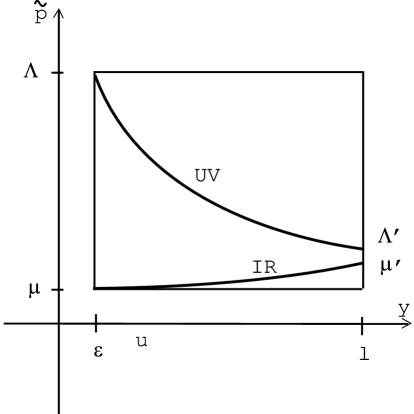
Figure 7: Space of (${\tilde{p}}$,y) for the integration (present proposal as the substitute of Fig.2).

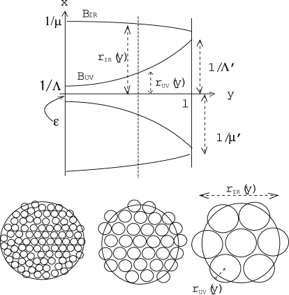
Figure 8: Regularization Surface $B_{IR}$ and $B_{UV}$ in the 5D coordinate space $(x^{\mu},y)$, Flow of Coarse Graining (Renormalization) and Sphere Lattice Regularization.

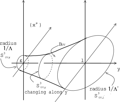
Figure 9: UV regularization surface in 5D coordinate space.

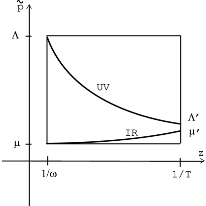
Figure 10: Space of (${\tilde{p}}$,z) for the integration (present proposal as the substitute of Fig.5).

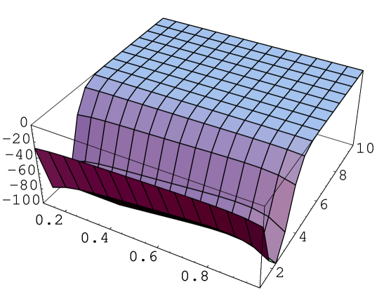
Figure 11: Behaviour of ${\tilde{p}}^{3}W_{1}({\tilde{p}},y)F({\tilde{p}},y)$(elliptic suppression). $\Lambda=10,\ l=1$ . $1/\Lambda\leq y\leq 0.99999l,\ 1/l\leq{\tilde{p}}\leq\Lambda$.

5 Introduction of the Weight Function $W({\tilde{p}},y)$ or $W({\tilde{p}},z)$

Another way to reduce the divergences is, instead of restriction, to introduce the weight function $W({\tilde{p}},y)$ or $W({\tilde{p}},z)$ in the integration over 5D space-time. The determination of the function form is explained later using the minimal area principle. Now we assume some forms as sample examples, and check whether Casimir energy is finitely obtained. For the flat case, we take the following forms.

$$W({\tilde{p}},y)=\mbox{\hskip 312.9803pt}$$

$$\left\{\begin{array}[]{cc}(N_{1})^{-1}\e^{-(1/2)l^{2}{\tilde{p}}^{2}-(1/2)y^{2}/l^{2}}\equiv W_{1}({\tilde{p}},y),\ N_{1}=1.557/8\pi^{2}&\mbox{elliptic suppression}\\ (N_{2})^{-1}\e^{-{\tilde{p}}y}\equiv W_{2}({\tilde{p}},y),\ N_{2}=2(l\Lambda)^{3}/8\pi^{2}&\mbox{hyperbolic suppression1}\end{array}\right.$$ (12)

$W_{2}$ is considered to imitate the Randall-Schwartz restriction. Fig.11 shows $W_{1}$-weighted case of Fig.2. We notice, in the ”valley”, the depth, the location and the shape change. The Casimir energy is numerically obtained as

$$E^{W}_{Cas}=\mbox{\hskip 284.52756pt}$$

$$\left\{\begin{array}[]{cc}-(2.500,2.501,2.501)\frac{\Lambda}{l^{3}}+(-0.142,1.09,1.13)\times 10^{-4}\frac{\Lambda\ln(l\Lambda)}{l^{3}}&\mbox{for}\quad W_{1}\\ -(6.0392,6.0394,6.03945)\times 10^{-2}\frac{\Lambda}{l^{3}}-(24.7,2.79,1.60)\times 10^{-8}\frac{\Lambda\ln(l\Lambda)}{l^{3}}&\mbox{for}\quad W_{2}\end{array}\right.$$ (15)

Triplet data show unstableness of the value due to insufficient range of $l$ and $\Lambda$. $\ln(l\Lambda)$ term vanishes for $W_{2}$ in the present calculational precision.

For the warped case. the situation goes similarly. We take the following weights.

$$W({\tilde{p}},z)=\hskip 142.26378pt$$

$$\left\{\begin{array}[]{cc}(N_{1})^{-1}\e^{-(1/2){\tilde{p}}^{2}/\omega^{2}-(1/2)z^{2}T^{2}}\equiv W_{1}({\tilde{p}},z),\ N_{1}=1.711/8\pi^{2}&\mbox{elliptic suppr.}\\ (N_{2})^{-1}\e^{-{\tilde{p}}zT/\omega}\equiv W_{2}({\tilde{p}},z),\ N_{2}=2\frac{\omega^{3}}{T^{3}}/8\pi^{2}&\mbox{hyperbolic suppr.1}\end{array}\right.$$ (18)

Fig.12 is W₁-weighted case of Fig.5. The ”valley” changes in its depth, shape and location. Casimir energy is given by

$$-E^{W}_{Cas}=\left\{\begin{array}[]{cc}\frac{\omega^{4}}{T}\Lambda\times 1.2\left\{1+0.11~{}\ln\frac{\Lambda}{\omega}-0.10~{}\ln\frac{\Lambda}{T}\right\}&\mbox{for}\quad W_{1}\\ \frac{T^{2}}{\omega^{2}}\Lambda^{4}\times 0.062\left\{1+0.03~{}\ln\frac{\Lambda}{\omega}-0.08~{}\ln\frac{\Lambda}{T}\right\}&\mbox{for}\quad W_{2}\end{array}\right.$$ (21)

For the hyperbolic case ($W_{2}$), the divergence is slightly milder than the case of RS-restriction (8) ($\Lambda^{5}\rightarrow\Lambda^{4}$). It is new that $\ln(\Lambda/T)$ appears.

After calculating for 13 different weights[15, 17], we conclude Casimir energy can be expressed as follows (except the hyperbolic weights). For the flat case,

$$E^{W}_{Cas}/\Lambda l=-\frac{\alpha}{l^{4}}\left(1-4c\ln(l\Lambda)\right){\quad.}$$ (22)

For the warped case

$$E^{W}_{Cas}/\Lambda T^{-1}=-\alpha\omega^{4}\left(1-4c\ln(\Lambda/\omega)-4c^{\prime}\ln(\Lambda/T)\right){\quad.}$$ (23)

The parameters $\alpha,c,c^{\prime}$ depend on the form of the chosen weight. The factors $\Lambda l$ and $\Lambda T^{-1}$ are the area of the rectangular regions (normalization constants). This result says the divergences of the 5D Casimir energy reduces to the log-divergence if we take into accout the weight properly. The final log-divergence can be renormalized into the boundary parameters $l$ (or $T$) and $\omega$. See Sec.8.

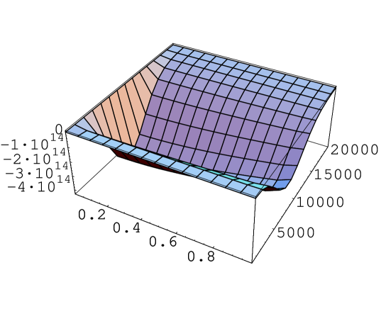
Figure 12: Behavior of $(-N_{1}/2){\tilde{p}}^{3}W_{1}({\tilde{p}},z)F^{-}({\tilde{p}},z)$(elliptic suppression). $\Lambda=20000,\ \omega=5000,\ T=1$ . $1.0001/\omega\leq z\leq 0.9999/T,\ \mu=\Lambda T/\omega\leq{\tilde{p}}\leq\Lambda$.

6 Meaning of Introduction of the Weight Function (1): Minimal Area Principle

In Ref.[19], we presented the following way to determine the form of $W$. Let us explain it in the warped case. $W({\tilde{p}},z)$ appears as

$$-E^{W}_{Cas}(\omega,T)={\int\frac{d^{4}p_{E}}{(2\pi)^{4}}}\int_{1/\omega}^{1/T}dz~{}W({\tilde{p}},z)F^{\mp}({\tilde{p}},z)$$

$$=\frac{2\pi^{2}}{(2\pi)^{4}}\int d{\tilde{p}}\int_{1/\omega}^{1/T}dz~{}{\tilde{p}}^{3}W({\tilde{p}},z)F^{\mp}({\tilde{p}},z){\quad.}$$ (24)

The integral region is the rectangular of Fig.10. We express the above expression by the following path-integral.

$$-E^{W}_{Cas}(\omega,T)=\int{\cal D}{\tilde{p}}(z)\int_{1/\omega}^{1/T}dz~{}S[{\tilde{p}}(z),z]\ ,$$

$$S[{\tilde{p}}(z),z]=\frac{2\pi^{2}}{(2\pi)^{4}}{\tilde{p}}(z)^{3}W({\tilde{p}}(z),z)F^{\mp}({\tilde{p}}(z),z).$$ (25)

All possible paths $\{{\tilde{p}}(z)|\omega^{-1}<z<T^{-1}\}$ are summed. The dominant contribution, in the above path-integral, is given by $\delta S=0$.

$$\mbox{Dominant Path }{\tilde{p}}_{W}(z)\ :\ \quad\frac{d{\tilde{p}}}{dz}=\frac{-\frac{\partial\ln(WF)}{\partial z}}{\frac{3}{{\tilde{p}}}+\frac{\partial\ln(WF)}{\partial{\tilde{p}}}}{\quad.}$$ (26)

This result says the dominant path ${\tilde{p}}_{W}(z)$ is determined by $W({\tilde{p}},z)$. A concrete example is the valley bottom line in Fig.12.

On the other hand, there exists another path which is determined independently of the above dominant path. That is the minimal area curve $r_{g}(z)$ which is given by

$$\mbox{Minimal Surface Curve }r_{g}(z)\ :\quad 3+\frac{4}{z}r^{\prime}r-\frac{r^{\prime\prime}r}{{r^{\prime}}^{2}+1}=0{\quad,}\quad\frac{1}{\omega}\leq z\leq\frac{1}{T}{\quad,}$$ (27)

where $r^{\prime}=\frac{dr}{dz},r^{\prime\prime}=\frac{d^{2}r}{dz^{2}}$. This differential equation is obtained by minimizing the area $A$ of the hyper-surface (9): $\delta A=0$ where $A$ is given by

$$ds^{2}=(\delta_{ab}+\frac{x^{a}x^{b}}{(rr^{\prime})^{2}})\frac{dx^{a}dx^{b}}{\omega^{2}z^{2}}\equiv g_{ab}(x)dx^{a}dx^{b},$$

$$A=\int\sqrt{\det g_{ab}}~{}d^{4}x=\int_{1/\omega}^{1/T}\frac{1}{\omega^{4}z^{4}}\sqrt{{r^{\prime}}^{2}+1}~{}r^{3}dz.$$ (28)

Hence this path $r_{g}(z)$ is determined by the induced geometry $g_{ab}(x)$. We require [15] the following relation in order to define $W({\tilde{p}},z)$.

$${\tilde{p}}_{W}(z)={\tilde{p}}_{g}(z)\ (=\frac{1}{r_{g}(z)}){\quad.}$$ (29)

In the above procedure, we have defined the integral measure $d^{4}p_{E}dzW({\tilde{p}},z)$ by the 5D bulk geometry or by the 4D induced geometry.

7 Meaning of Introduction of the Weight Function (2): Fluctuation of Space-Time

For the purpose of naturally introducing the idea of the previous sections, we newly define Casimir energy in the higher dimension by the following generalized path-integral. (warped case).

$$-{\cal E}_{Cas}(\omega,T,\Lambda)\equiv\int_{1/\Lambda}^{1/\mu}d\rho\int_{\begin{array}[]{l}r(1/\omega)\\ =r(1/T)\\ =\rho\end{array}}\prod_{a,z}{\cal D}x^{a}(z)\times$$ (33)

$$F(\frac{1}{r},z)~{}\exp\left[-\frac{1}{2\alpha^{\prime}}\int_{1/\omega}^{1/T}\frac{1}{\omega^{4}z^{4}}\sqrt{{r^{\prime}}^{2}+1}~{}r^{3}dz\right],$$ (34)

where $\mu=\Lambda T/\omega$ is the IR-cutoff parameter, and we take the limit $\Lambda T^{-1}\rightarrow\infty$ at the final stage. $1/2\alpha^{\prime}$ is the string (surface) tension parameter ($\alpha^{\prime}$ has the dimension of [Length]⁴). $F({\tilde{p}},z)$ comes from the quantum fluctuation of the bulk matter field.

The above path-integral expression says the 4D coordinates $x^{a}$ play the role of operators of the quantum statistical mechanics [20]. The extra coordinate $z$ is the parameter of the inverse temperature. It looks that the space-time coordinates are fluctuating.

We expect the numerical or analytical evaluation of Casimir energy (34) directly gives similar results explained so far.

8 Conclusion

We show, in Fig.13, the Planck’s radiation distribution in the stereo-graphical way by adding the inverse temperature axis. The behavior looks similar to Fig.12 except the sign. It says the extra coordinate corresponds to the inverse temperature.

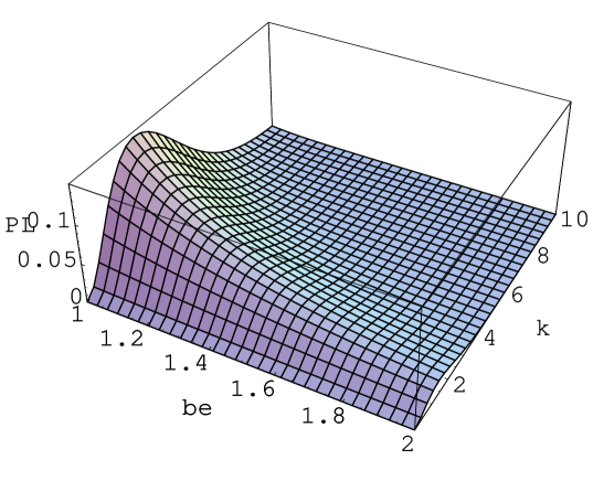
Figure 13: Graph of Planck’s radiation formula. ${\cal P}(\beta,k)=\frac{1}{(c\hbar)^{3}}\frac{1}{\pi^{2}}k^{3}/(\e^{\beta k}-1)\ \ (1\leq\beta\leq 2,\ 0.01\leq k\leq 10)$.

The log-divergences in Casimir energy (22) and (23) are familiar in the quantum field theory. For the warped case, they are renormalized into the boundary parameter $\omega$.

$$\frac{E^{W}_{Cas}}{\Lambda T^{-1}}=-\alpha\omega^{4}\left(1-4c\ln(\frac{\Lambda}{\omega})-4c^{\prime}\ln(\frac{\Lambda}{T})\right)=-\alpha(\omega_{r})^{4}{\quad,}$$

$$\omega_{r}=\omega\sqrt[4]{1-4c\ln(\frac{\Lambda}{\omega})-4c^{\prime}\ln(\frac{\Lambda}{T})}{\quad.}$$ (35)

Local counterterms are unnecessary. Divergences are directly absorbed into the boundary parameter. Note that $c$ and $c^{\prime}$ are pure numbers and represent the interaction between the bounaries and the (free) field. Compare this with the ordinary renormalization, like QED, where the $\beta$-function depends on the coupling. When $c$ and $c^{\prime}$ are sufficiently small, the $\beta$-function is given as

$$|c|\ll 1\ ,\ |c^{\prime}|\ll 1{\quad,}\quad\omega_{r}=\omega(1-c\ln(\Lambda/\omega)-c^{\prime}\ln(\Lambda/T)){\quad,}$$

$$\beta\equiv\frac{\partial}{\partial(\ln\Lambda)}\ln\frac{\omega_{r}}{\omega}=-c-c^{\prime}{\quad.}$$ (36)

The scaling behavior of $\omega$ is determined by the sign of $c+c^{\prime}$. Because we identify Casimir energy (35) with the cosmological constant, the sign also determines the scaling behavior of the constant. Note that the direction of flow, which determines the attractive or repulsive force, is not given by the derivative (w.r.t. the boundary parameter) of Casimir energy.

For the flat case (22), the other boundary parameter $l$ is renormalized[15].

Parameters, which appears in the 5D warped model, can be fitted in the way consistent with the present observation (except the sign). First we take the 4D momentum cut-off $\Lambda=M_{pl}\sim 1.2\times 10^{19}$GeV. The present final result (35) says $|S(\mbox{Euclidian Action})|\sim{\int d^{4}x}\sqrt{-g}\lambda_{obs}/G_{N}\propto\omega^{4}$. The observational data says $|S(\mbox{Euclidian Action})|\sim{\int d^{4}x}\sqrt{-g}\lambda_{obs}/G_{N}\sim(R_{cos})^{4}(10^{-3}\mbox{eV})^{4}$ where $R_{cos}\sim 5.\times 10^{41}$GeV^-1 is the size of the present universe. The experimental result about the Newton’s gravitational force tells us the warped parameter $\omega$ is taken as $\omega\sim 10^{-3}$eV. Note that $\omega\sim\sqrt{M_{pl}/R_{cos}},~{}R_{cos}\cdot\omega\sim\sqrt{M_{pl}\cdot R_{cos}}=\sqrt{N_{DL}}$. Hence $|S(\mbox{Euclidian Action})|\sim{N_{DL}}^{2}=4.\times 10^{121}$. From (35), $|E_{Cas}|\sim\Lambda T^{-1}\omega^{4}$. We can identify $T^{-4}|E_{Cas}|\sim\Lambda T^{-5}\omega^{4}$ with $|S(\mbox{Euclidian Action})|\sim(R_{cos})^{4}\omega^{4}$. Hence $T\sim{R_{cos}}^{-1}{N_{DL}}^{1/5}\sim 3.\times 10^{-30}$GeV. $\mu=\Lambda T/\omega\sim M_{pl}{N_{DL}}^{-3/10}\sim 7.$ GeV. The IR cutoff $\mu$ is near to the nucleon mass or the weak boson mass. If we interpret, in Fig.8, the number of small 4D balls within the S³ boundary is the degree of freedom of the present system, then it is grossly given by $\Lambda^{4}/\mu^{4}=\omega^{4}/T^{4}\sim{N_{DL}}^{6/5}\sim 9.\times 10^{72}$. Finally we note the neutrino mass, $m_{\nu}$, is similar to the warp parameter (5D bulk curvature) $\omega$.

As stated in Sec.7, the present formulation of the higher dimensional quantum field theory gives the picture of the fluctuating space-time. It is known, in the string theory, the uncertainty principle appears in the space-time coordinates[21].

9 Acknowledgment

The past development is given in the proceedings of some conferences[22, 23, 24, 25, 26]. The author thanks the audience.

References

- [1] S. Weinberg, Rev.Mod.Phys.61(1989)1
- [2] T. Padmanabhan, Phys.Rept.380(2003)235
- [3] A.M. Polyakov, Sov.Phys.Usp.25(1982)187 [Usp.Fiz.Nauk 136(1982)538]
- [4] A.M. Polyakov, Nucl.Phys.B797(2008)199, arXiv:0709.2899(hep-th)
- [5] A.M. Polyakov, Nucl.Phys.B834(2010)316, arXiv:0912.5503
- [6] I. Bredberg, C. Keeler, V. Lysov and A. Strominger, ”From Navier-Stokes To Einstein”, arXiv: 1101.2451(hep-th)
- [7] V. Lysov and A. Strominger, ”From Petrov-Einstein to Navier-Stokes”, arXiv: 1104.5502(hep-th), 2011
- [8] R.P. Feynman, Acta Phys. Polonica24(1963)697
- [9] G. ’tHooft and M. Veltman, Ann. Inst. Henri Poincaŕe 20(1974)69
- [10] E. Witten, ”Quantum Gravity IN De Sitter Space”, arXiv: hep-th/0106109, 2001
- [11] Erik Verlinde, JHEP1104:029, 2011, arXiv:1001.0785
- [12] T. Jacobson, Phys.Rev.Lett.75(1995)1260, arXiv:gr-qc/9504004
- [13] T. Padmanabhan, Rep.Prog.Phys.73(2010)046901, arXiv:0911.5004
- [14] P.A.M. Dirac, Nature 139(1937)323; Proc.Roy.Soc.A165(1938)199; ”Directions in Physics”, John Wiley & Sons, Inc., New York, 1978
- [15] S. Ichinose,Prog.Theor.Phys.121(2009)727, ArXiv:0801.3064v8[hep-th].
-
[16]
T. Appelquist and A. Chodos, \PRD28(1983)772
T. Appelquist and A. Chodos, \PRL50(1983)141 - [17] S. Ichinose, ”Casimir Energy of 5D Warped System and Sphere Lattice Regularization”, ArXiv:0812.1263[hep-th], US-08-03.
- [18] L. Randall and M.D. Schwartz, JHEP 0111 (2001) 003, hep-th/0108114
- [19] S. Ichinose and A. Murayama, \PRD76(2007)065008, hep-th/0703228
- [20] R.P. Feynman, ”Statistical Mechanics”, W.A. Benjamin, Inc., Massachusetts, 1972
-
[21]
T. Yoneya, Duality and Indeterminacy Principle in String Theory in ”Wandering in the Fields”,
eds. K. Kawarabayashi and A. Ukawa (World Scientific,1987), p.419
T. Yoneya, String Theory and Quantum Gravity in ”Quantum String Theory”, eds. N. Kawamoto and T. Kugo (Springer,1988), p.23
T. Yoneya, Prog.Theor.Phys.103(2000)1081 - [22] S. Ichinose, Proc. of VIII Asia-Pacific Int. Conf. on Gravitation and Astrophysics (ICGA8,Aug.29-Sep.1,2007,Nara Women’s Univ.,Japan),Press Section p36-39, arXiv:/0712.4043
- [23] S. Ichinose, Int.Jour.Mod.Phys.23A(2008)2245-2248, Proc. of Int. Conf. on Prog. of String Theory and Quantum Field Theory (Dec.7-10,2007,Osaka City Univ.,Japan), arXiv:/0804.0945
- [24] S. Ichinose, Int.Jour.Mod.Phys.24A(2009)3620, Proc. of Int. Conf. on Particle Physics, Astrophysics and Quantum Field Theory: 75 Years since Solvay (Nov.27-29, 2008, Nanyang Executive Centre, Singapore), arXiv:0903.4971
- [25] S. Ichinose, Jour.Phys.:Conf.Scr.222(2010)012048. ArXiv:1001.0222[hep-th], Proc. of First Mediterranean Conference on Classical and Quantum Gravity (09.9.14-18, Kolymbari, Crete, Greece),
- [26] S. Ichinose, Proc. of Int. Workshop on ’Strong Coupling Gauge Theories in LHC Era’(09.12.8-11, Nagoya Univ., Nagoya, Japan), editted by H. Fukaya et al, p407 (World Scientific). arXiv:1003.5041(hep-th).