Testing a hypothesis of the $\nu$ Octantis planetary system

Abstract

We investigate the orbital stability of a putative Jovian planet in a compact binary $\nu$ Octantis reported by Ramm et al. We re-analyzed published radial velocity data in terms of self-consistent Newtonian model and we found stable best-fit solutions that obey observational constraints. They correspond to retrograde orbits, in accord with an earlier hypothesis of Eberle & Cuntz, with apsidal lines anti-aligned with the apses of the binary. The best-fit solutions are confined to tiny stable regions of the phase space. These regions have a structure of the Arnold web formed by overlapping low-order mean motion resonances and their sub-resonances. The presence of a real planet is still questionable, because its formation would be hindered by strong dynamical perturbations. Our numerical study makes use of a new computational Message Passing Interface (MPI) framework Mechanic developed to run massive numerical experiments on CPU clusters.

1 Introduction

The $\nu$ Octantis is a single–line spectroscopic binary composed of the $\nu$ Oct A K1 III giant primary ($1.4\pm 0.3$ M_⊙) and an unseen red dwarf secondary $\nu$ Oct B, K7-M1 V ($0.5\pm 0.1$ M_⊙) separated by $\sim 2.55\pm 0.13$ au. Colacevich (1935) collected 11 radial velocities (RVs) of the primary, and Alden (1939) determined the astrometric orbit. Recently, the orbital period $P_{\mbox{\scriptsize bin}}=1050.11\pm 0.13$ days and eccentricity $e_{\mbox{\scriptsize b}}=0.2358\pm 0.0003$ were determined by Ramm et al. (2009). Remarkably, they also derived the inclination $i_{\mbox{\scriptsize bin}}=71^{\circ}$ with an error less than $1^{\circ}$ on the basis of Hipparchos astrometry and new 223 precision RVs. Ramm et al. (2009) discovered residual variability of these RVs at a level of $\sim 200$ $\mbox{ms}^{-1}$ and explained this by an S-type (Dvorak, 1984) Jovian planet , $\nu$ Oct Ab , having a minimal mass $m_{\mbox{\scriptsize p}}\sin i_{\mbox{\scriptsize p}}=2.5$ m${}_{\mbox{\scriptsize Jup}}$ in an orbit with a semi-major axis $a_{\mbox{\scriptsize p}}=1.2\pm 0.1$ au and an eccentricity $e_{\mbox{\scriptsize p}}=0.123\pm 0.037$.

The putative planet is unusual, because the derived semi-major axis implies its orbit roughly in the middle between massive primary and secondary. A formation of such a planet in the compact binary can be hardly explained (e.g., Kley, 2010). Analytic or general stability criteria formulated for the restricted and general three-body problem like the Hill stability criterion, the results of Holman & Wiegert (1999), or the resonance-overlap criterion by Wisdom (1983) are violated if the planet is assumed to be in a prograde orbit. According with the determination of stability limits in binaries (Holman & Wiegert, 1999), a coplanar, prograde planetary configuration might be stable only up to astrocentric distance $\sim 0.64$ au (Ramm et al., 2009). Indeed, Eberle & Cuntz (2010) found that the Keplerian best-fit model in the discovery paper is strongly unstable in just 1–10 binary periods time-scale for the case of prograde motion. This contradicts the planetary hypothesis, although the discovery paper basically excludes non-planetary sources of the observed signal, like stellar spots or pulsations.

Many explanations of the observed RVs variability are still possible, which might resolve the apparent paradox of the strongly unstable system. The residual RVs may be implied by stellar chromospheric activity, a different number of planetary companions, systematic errors of the observations, instrumental instabilities and non-Gaussian uncertainties, such as the red noise (Baluev, 2011), or a different orbital model than the configuration in the discovery paper. Indeed, Morais & Correia (2012) consider a hierarchical triple system with an unseen binary in the place of secondary $\nu$ Oct B. Such an orbital setup forces a precession of the primary orbit around the barycentre of the inner binary and it could mimic the RV variations attributed to the putative planet.

Earlier, Eberle & Cuntz (2010) following the stability studies of the restricted three body problem by Jefferys (1974) found that a retrograde orbit of the planet lies in much wider stable zone than the direct configuration. In a new work, Quarles et al. (2012) investigate this model, extending the set of orbital configurations, through a numerical study in the framework of the elliptic, restricted three-body problem.

In more than a decade, modeling the precision RVs teaches us that the dynamical analysis of the $\nu$ Octantis system done in the discovery paper (Ramm et al., 2009), and following studies (Eberle & Cuntz, 2010; Quarles et al., 2012) do not seem fully consistent with its dynamical character. Because the secondary mass may be almost a half of the primary mass, the relatively wide planetary orbit is strongly perturbed. The perturbation parameter, expressed by the mass ratio of the binary, can be as large as $\sim$0.38 (Ramm et al., 2009). In such a case the mutual interactions are important to compute the RV signal (Laughlin & Chambers, 2001). Furthermore, it was assumed that the whole system is co-planar, no matter if the planetary orbit is prograde or retrograde. However, non-planar orbits in compact binaries might appear due to violent post–formation scenarios due to the planet–planet scattering (e.g., Adams & Laughlin, 2003). This may imply highly inclined configurations and their dynamics much complex than in a coplanar case (e.g., Migaszewski & Goździewski, 2011). The dynamical simulations done by Eberle & Cuntz (2010) concern initially aligned orbits. Quarles et al. (2012) study a system with initial planetary eccentricity $e_{\mbox{\scriptsize p}}=0$ and two initial longitudes ${\lambda}_{\mbox{\scriptsize p}}=0^{\circ}$,$180^{\circ}$, respectively (corresponding to 3 o’clock and 9 o’clock positions in their terminology). While a particular initial orientation of the orbits may be protecting factor for the stability, the initial orbital phases should not be fixed or selected a’priori, if the tested configuration is meant to be consistent with the observations, where we aim to analyze the dynamics of a real system. As a simple example, consider Keplerian RV signal computed from the well known formulae $RV(\nu)=K[\cos(\omega+\nu)+e\cos(\omega)],$ where $K$ is the semi-amplitude, $\omega$ is for the pericenter argument of the orbit, $e$ is the eccentricity and $\nu$ is the true anomaly. Function $RV(\nu)$ changes its sign, if instead of $\omega=0^{\circ}$ one sets $\omega=180^{\circ}$ at the initial time. Obviously, a more complex modification of $RV(\nu)$ is introduced if other angles are altered, such as orbital longitudes. In general, the initial orbital configuration determines the dynamical evolution and the reflex motion of the primary, which should be consistent with observations.

In this work, we aim to verify and improve the kinematic (Keplerian) model of the $\nu$ Oct planetary system by searching for the best-fit configurations in terms of self-consistent dynamical, $N$-body model (Laughlin & Chambers, 2001, and references therein). To resolve the fine structure of the phase space, and to investigate the dynamics and long–term stability of the planet, we apply the fast-indicator MEGNO (Cincotta et al., 2003) adapted to our new multi-CPU computing environment Mechanic. In this paper, we demonstrate a non-trivial application of this software. It was announced by Słonina et al. (2012). The Mechanic code is described in an accompanying work to this paper (Słonina et al., in preparation), and is freely available on-line (http://git.ca.umk.pl).

This paper is structured as follows. After this introduction, section 2 is devoted to the dynamical analysis of orbital solution proposed in (Eberle & Cuntz, 2010) to possibly global extent. We attempt to visualize complex resonant structures in the vicinity of presumable retrograde planetary configurations. This part has a general character, because we analyze unstable behaviours of S-type planets in compact binaries. In the next section 3, we focus on an re-analysis of the RV observations and on deriving the best-fit parameters of the $\nu$ Oct system in terms of three distinct models of the RV: the Keplerian (kinematic) formulation, Newtonian (dynamic) model, and the Newtonian model with stability constraints (GAMP, Goździewski et al., 2008). In section 4 we demonstrate that stable, retrograde orbits consistent with the RVs data may be found, indeed, but these three RV models lead to significantly different orbital architectures. Conclusions are given in section 5.

2 The dynamics of the $\nu$ Octantis system

To resolve the paradox of the $\nu$ Octantis system instability, Eberle & Cuntz (2010) searched for stable orbits at a grid of primary mass ($1.1,1.4$ and $1.7$)  M_⊙, three mass ratios ($\mu$ = $0.2593,0.2754$, $0.2908$), and 30–step initial distance ratio $\rho$ between the planet and the secondary, $\rho\in\langle 0.22,0.54\rangle\equiv\langle 0.56,1.38\rangle$ au. The equations of motion were integrated for $10^{3}$ years ($\sim$ 350 binary periods $P_{\mbox{\scriptsize bin}}$) for prograde orbits, and for $1\times 10^{4}$  years ($\sim$ 3500 $P_{\mbox{\scriptsize bin}}$) for retrograde orbits. The initial orbits were aligned with both secondaries fixed in their apoastrons with respect to the primary. These integrations confirmed the theoretical stability limit $\rho\sim 0.25\equiv 0.64$ au for prograde orbits in (Holman & Wiegert, 1999). For the retrograde case, the stability limit was found much larger, indeed, $\rho\sim 0.479$ consistent with the formal $3\sigma$ best-fit error in (Ramm et al., 2009).

2.1 Stability of a system with initially aligned apsides

To extend the study of Eberle & Cuntz (2010), we applied the dynamical maps technique. It helps to illustrate the global structure of the phase space, as well as to identify possible resonances as the origin of strong instability observed in this system. We use MEGNO which is a measure of the maximal Lyapunov exponent (Cincotta et al., 2003) as the stability indicator. Our serial-CPU software to integrate the equations of motions and the variational equations of the planetary problem was encapsulated in the Mechanic MPI module called the CSM. A strongly interacting planetary system with collisional orbits requires an appropriate integrator. We applied the Bulirsh-Stoer-Gragg scheme implemented as reliable and well tested ODEX routine (Hairer et al., 1993). It provides very good accuracy and performance (see also, Chambers, 1999). The total integration time of a single initial condition was not less than $10^{4}$ periods of the binary, and in some cases more than $3\times 10^{5}$ periods. This time is typically one–two orders of magnitude longer than the time-span of direct numerical integrations in Eberle & Cuntz (2010), and provides at least $10$-$100$ longer estimate of the Lagrange stability, in accord corrwith features of MEGNO (Cincotta et al., 2003). The time scale of MEGNO integrations is long enough to detect most significant mean motion resonances (Goździewski et al., 2008).

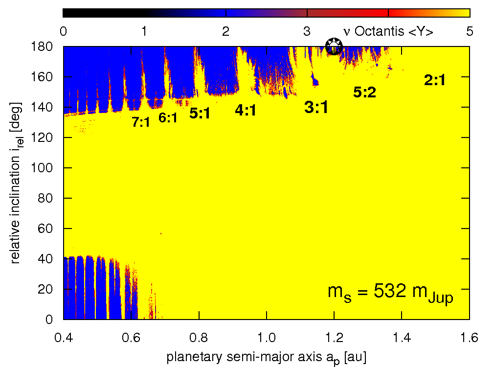
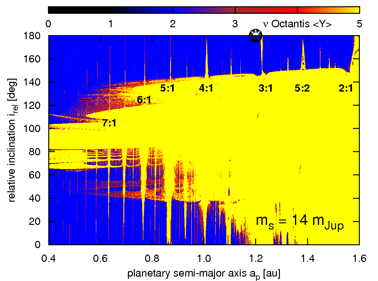
Figure 1: MEGNO dynamical maps for the geometric setup of the $\nu$ Octantis planetary system investigated by Eberle & Cuntz (2010). The initial apsidal lines of the orbits are aligned. A reference position of the planet in the discovery paper by Ramm et al. is marked with an asterisk. The low-order mean motion resonances between the planet and the secondary are labeled. The left panel is for the global view of the phase space for the nominal mass of the secondary, the right panel is for an artificial brown dwarf secondary, helpful to identify the MMRs. The raw resolution is $1440\times 900$ initial conditions integrated for $\sim 3\times 10^{4}$ periods of the binary.

In the first numerical experiment, we set the primary mass to $1.4$ M_⊙ which is equivalent to $\mu=0.28$. In accord with Eberle & Cuntz (2010), the planet and the secondary are placed in the apoastrons of their orbits, hence the initial mean anomalies ${\cal M}_{\mbox{\scriptsize p}}={\cal M}_{\mbox{\scriptsize S}}=180^{\circ}$, of the planet and the secondary, respectively. Arguments of periastrons and the nodal longitudes were set to $0^{\circ}$. In the following numerical experiments, we varied the inclination of the planet (equivalent to the relative inclination of the orbits) between $i_{\mbox{\scriptsize p}}=0^{\circ}$ (direct coplanar configuration) and $i_{\mbox{\scriptsize p}}=180^{\circ}$ (retrograde coplanar configuration). This setup, which we consider as aligned orbits, reproduces the initial configurations in Eberle & Cuntz (2010), i.e., the 9 o’clock position in their terminology. We computed MEGNO maps in high-resolution with a grid of $1440\times 900$ pixels that were integrated for 25,000 periods of the binary. The results are illustrated in Fig. 1, in the semi–major axis $a_{\mbox{\scriptsize p}}$ — relative inclination $i_{\mbox{\scriptsize rel}}$–plane for the two secondary masses. The right map is for an artificial brown dwarf secondary, to illustrate, through a comparison, the strength of the perturbation in the nominal $\nu$ Oct system (the left panel in Fig. 1). For prograde configurations, the stability limit $a_{\mbox{\scriptsize p}}\sim 0.6$ au is slightly smaller than its value found in the previous papers. For retrograde orbits, it is almost doubled and reaches $a_{\mbox{\scriptsize p}}\sim 1.2$ au. A putative planet could be located at a border of this zone, filled with unstable low-order MMRs. A stable retrograde orbit found by Eberle & Cuntz (2010) lies in a region spanned by strong 4:1, 3:1, 5:2 and 2:1 MMRs. A close-up of this area covering the 5:2 MMR, slightly beyond the semi-major axis of the planet determined in (Ramm et al., 2009), is shown in Fig. 2. Overlapping of the MMRs and their sub-resonances creates a global chaotic zone. This effect is identified as the main source of instability of planets in compact binaries (Mudryk & Wu, 2006).

The stability limit depends strongly on the relative inclination and the mass of the secondary. Configurations with intermediate relative inclinations, roughly between $\sim 40^{\circ}$ and $\sim 140^{\circ}$, and particularly solutions close to polar orbits ($i_{\mbox{\scriptsize rel}}\sim 90^{\circ}$) are very chaotic. They are associated with the Kozai resonance (Kozai, 1962), see also section 2.3. For non-coplanar orbits, the border of stable zone may be much closer to the primary than 0.4 au. Even for a hypothetical, low–mass secondary $\sim$14 m${}_{\mbox{\scriptsize Jup}}$ (Fig. 1, right panel), polar orbits are very unstable. In this case, stable prograde solutions may be found up to $\sim 1.2$ au. We also note that individual unstable MMRs are much wider for prograde orbits than for retrograde configurations. A theoretical explanation of this phenomenon is given in a recent paper by Morais & Giuppone (2012). The stability limits are governed by the phase-space topology of retrograde and prograde MMRs. At the $p$/$q$ mean motion ratio, the prograde resonance is of order $p-q$ while the retrograde resonance is of order $p+q$, hence the resonance order is higher. Although this result is derived for the circular, restricted three body problem, it should be valid also for small–eccentricity binaries. This is confirmed by Fig. 1 showing different widths of prograde and retrograde MMRs for $e_{\mbox{\scriptsize bin}}\simeq 0.123$.

2.2 Developing the instability with the secondary mass

An identification of the origin of instabilities for large mass ratio of the binary is not straightforward. Due to overlapping MMRs and their sub-resonances, a complex pattern of stable and unstable motions appears (compare panels in Fig. 1). To study how the unstable zones are evolved with increasing perturbation, we performed a numerical experiment in which the secondary mass was gradually increased from an artificial value of 14 m${}_{\mbox{\scriptsize Jup}}$ (a brown dwarf, see the right panel in Fig. 1), up to the nominal value of 532 m${}_{\mbox{\scriptsize Jup}}$ (the left panel of Fig. 1). For the small mass secondary, the MMRs can be easily identified, and we can follow, how they expand when the perturbation of the secondary grows. In this way, we may also refer to a low-dimensional dynamical system given through model Hamiltonian in Froeschlé et al. (2000). The dynamics of the S-type planet in the binary should reveal qualitatively similar features because this is also governed by a perturbed Hamiltonian of the form ${\cal H}={\cal H}_{0}+\epsilon{\cal H}_{1}$, where ${\cal H}_{0}$ is the integrable (Keplerian) part, and ${\cal H}_{1}$ is the perturbation due to mutual interactions of the planet and the binary. The perturbation parameter $\epsilon$ can be expressed through $\epsilon\sim m_{\mbox{\scriptsize S}}/m_{\mbox{\scriptsize P}}\equiv\mu,$ where $m_{\mbox{\scriptsize S}}$ is the mass of the secondary companion $\nu$ Oct B and $m_{\mbox{\scriptsize P}}$ is the mass of the primary $\nu$ Oct A.

The results are illustrated through a sequence of dynamical maps in Fig. 3. These MEGNO maps were computed for $\sim 10^{4}$ periods of the binary. At each panel, we labeled the lowest-order MMRs and the mass of the secondary (perturber). Each Mechanic run occupied 256 CPUs, and computations took, depending on initial conditions (an extent of the chaotic zone) up to a few hours of CPU time. Already for the smallest mass ratio, corresponding to brown dwarf mass perturber, a large part of the phase space is strongly chaotic (the top-left panel of Fig. 3, also the right panel in Fig. 1). In the relevant zone of retrograde motions, a pattern of narrow MMRs appears. A retrograde orbit might have much more stable space to explore than a direct orbit. In this regime, the probability of a stable orbit would be close to 1. When the perturber mass is increased, the widths of MMRs quickly expand, and for $m_{\mbox{\scriptsize S}}\sim 380$ m${}_{\mbox{\scriptsize Jup}}$ (roughly, the left mass limit of the secondary) one may observe that strong MMRs are overlapping which emerges a zone of global chaos, roughly beyond $a_{\mbox{\scriptsize p}}\sim 1.2$  au. For the nominal mass of the perturber (see the bottom right panel in Fig. 3), there are only narrow areas of stable motions.

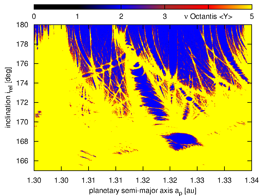
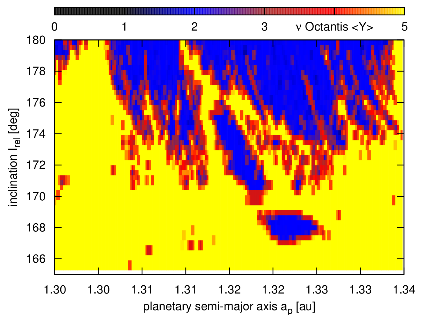
Figure 2: A close up of the MEGNO dynamical map for the orbital configuration with apsidal lines initially aligned, in a neighborhood of the formal best-fit model in (Ramm et al. 2009). The resolution of the left panel is $1440\times 900$ pixels and, for a reference, the right panel has the resolution of $200\times 50$ pixels. Each initial condition was integrated for $\sim 3\times 10^{4}$ and $\sim 10^{4}$ periods of the binary, respectively.

A close-up of that region in Fig. 2 demonstrates a view of the phase space of the model Hamiltonian for large perturbation parameter $\epsilon$ (Froeschlé et al., 2000), see also (Słonina et al., 2012). The fine structures seen in this map represent the Arnold web in the three body problem. They appear due to overlapping MMRs and their sub-resonances, strongly split by the perturbation. This feature is expected because it was found in the Outer Solar system (Guzzo, 2005) and, very recently, in the Kepler-11 extrasolar system of six planets (Migaszewski et al., 2012). Likely, it has not been shown in the three body problem with so much details. The right panel of Fig. 2 shows the MEGNO map in the same area, but with lower resolution of $200\times 50$ pixels, computed for $1\times 10^{4}$ periods of the binary. We see that a fine resolution $1440\times 900$ pixels, as well as longer integration time $\sim 3\times 10^{4}$ P${}_{\mbox{\scriptsize bin}}$ are crucial to discover the fine details of the phase space. ( See section 4 for more examples of such structures in the neighborhood of the Newtonian best-fit model of the $\nu$ Octantis system, consistent with available observations).

The dynamical stability of planetary orbits in systems exhibiting strong mutual interactions can be influenced even by very small changes of the initial conditions due to the presence of unstable resonances and their overlapping. If the mutual perturbations are small enough, and chaotic motions appear on a regular net, they may be practically stable over very long times (Guzzo, 2005). Such a state of the system is called the Nekhoroshev regime. Otherwise, if the chaotic motions do not constitute a regular web, and most of orbits form a global chaotic zone, the stability of the system is influenced by a strong chaotic diffusion. This regime is related to the resonance overlapping, and is called the Chirikov regime (Froeschlé et al., 2000; Guzzo, 2005).

The Arnold web emerging due to three–body and four–body MMRs was investigated by Guzzo (2005, 2006) in the Outer Solar system. He mapped the phase space in the semi-major axes planes of Jupiter, Saturn, Uranus and Neptune. Here, we illustrate this feature in the three–body problem in the semi-major axis — inclination plane, corresponding to a different choice of the canonical actions, and appearing due to two–body MMRs. The Arnold web creates an intermediate zone between the ordered and strongly chaotic motions, which spans relatively wide range of the inclination, extending for $10^{\circ}$. In this intermediate region, the phase-space motions which are chaotic, may persist over long periods of time. The results of this experiment also show that the stability limits for co-planar binaries derived numerically by Holman & Wiegert (1999) may be strongly affected by the inclination. In our case of moderate eccentricity of the planetary orbit, these limits are roughly valid for $i_{\mbox{\scriptsize rel}}\in(0^{\circ},40^{\circ})$ and $i_{\mbox{\scriptsize rel}}\in(140^{\circ},180^{\circ})$. A determination of stability limits in systems with non-zero relative inclinations needs additional extensive numerical study recalling that our computations concern a particular initial configuration of the orbits. We postpone this subject to a new work.

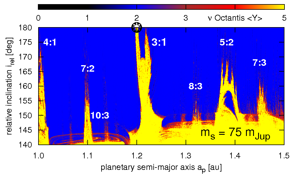
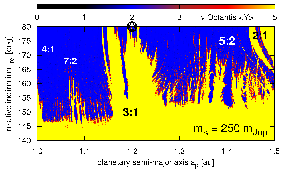
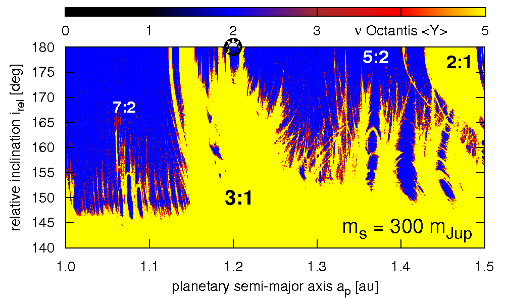
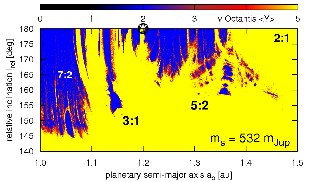
Figure 3: The results of a numerical experiment in which the secondary mass was gradually increased from 14 m${}_{\mbox{\scriptsize Jup}}$ (the top left panel), through 75 m${}_{\mbox{\scriptsize Jup}}$, 150 m${}_{\mbox{\scriptsize Jup}}$, 250 m${}_{\mbox{\scriptsize Jup}}$, 300 m${}_{\mbox{\scriptsize Jup}}$, 380 m${}_{\mbox{\scriptsize Jup}}$, 462  m${}_{\mbox{\scriptsize Jup}}$, up to the nominal mass 532 m${}_{\mbox{\scriptsize Jup}}$ of the $\nu$ OctantisB (the bottom right panel). Initial geometric configuration is fixed the same as in the retrograde orbit model by Eberle & Cuntz (2010). A reference position of the planet is marked with an asterisk. Most significant MMRs between the planet and the secondary are labeled. The MEGNO integration time is $\sim 1\times 10^{4}$ periods of the binary.

2.3 The secular dynamics of the planet

The origin of a wide strip of unstable motions around polar orbits can be explained with the help of the secular octupole–level theory (e.g., Migaszewski & Goździewski, 2011, and references therein). For a direct comparison with the MEGNO integrations, we focus again on the initial orbital setup in (Eberle & Cuntz, 2010). For small $a_{\mbox{\scriptsize p}}\sim 0.6$ au and less, the expansion parameter $\alpha=a_{\mbox{\scriptsize p}}/a_{\mbox{\scriptsize bin}}\sim 0.25$ where the system may be considered as non-resonant. This permit us to study the long–term dynamics through the secular theory. The range of $a_{\mbox{\scriptsize p}}\in[0.4,1.2]$ au is investigated to compare both relevant intervals of direct and retrograde motion although $\alpha$ becomes as large as $0.5$ at the right border of this interval and the assumptions of the secular theory may be questionable.

The results are illustrated in Fig. 4 in the form of dynamical maps in the $(a_{\mbox{\scriptsize p}},i_{\mbox{\scriptsize rel}}$)–plane. The left column is for the nominal mass of $\nu$ Oct B, and the right column is for an artificial, low-mass secondary of $14$ m${}_{\mbox{\scriptsize Jup}}$. The top row illustrates the maximal eccentricity attained by the planet over the secular orbital period. Both perturbers are massive enough to force extreme eccentricity $\sim 1$. This must imply collisions with the primaries. Indeed, in the middle panels showing the maximum apocenter distance of the planet, the filled dots mark initial conditions that led to a collision with the star. These two zones closely coincide. If the initial semi-major axis is increased, the minimum distance of the planet to the secondary becomes almost always close to 0 au (see the bottom row in Fig. 4). Filled dots in these panels mark regions, in which angle $\Delta\varpi\equiv\varpi_{\mbox{\scriptsize p}}-\varpi_{\mbox{\scriptsize S}}$ librates.

This experiment reveals that a continuous unstable zone between $i_{\mbox{\scriptsize rel}}\in(40^{\circ},140^{\circ})$ predicted by the secular model closely coincides with unstable region around the polar orbits exhibited in the full three-body system. It means that this unstable region appear due to the Kozai resonance which is able to force large eccentricities in the secular time-scale. More details and a concise description of the Kozai resonance in the context of planetary dynamics may be found in a recent review (Beaugé et al., 2012, p. 1065–1068, and references therein). Hence the primary source of instability can be identified with a secular effect rather than with short-term chaotic dynamics associated with the MMRs. Outside unstable zones of the Kozai resonance, the primary source of instability are the MMRs which appear as discrete areas of chaos for small value of the perturbation parameters, and a zone of global chaos when the perturbation becomes sufficiently strong and the short-term MMRs may govern the global dynamics. Let us note, that although the global picture of the secular system is illustrated here for the aligned configuration, it remains qualitatively the same for the anti-aligned orbits.

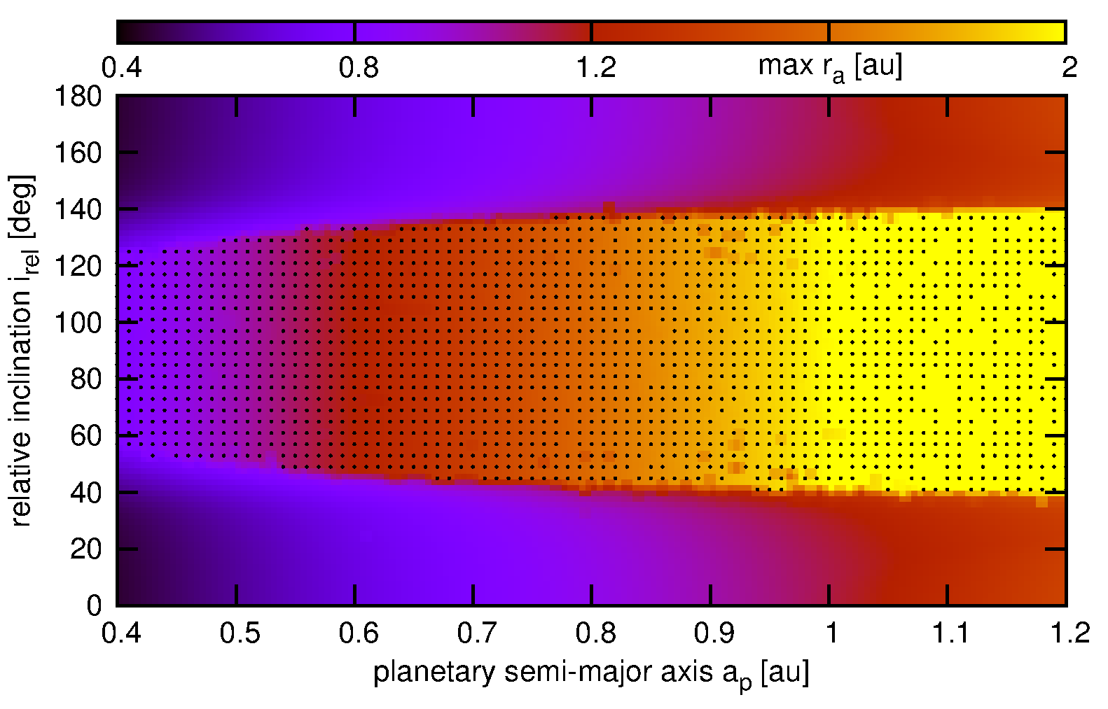
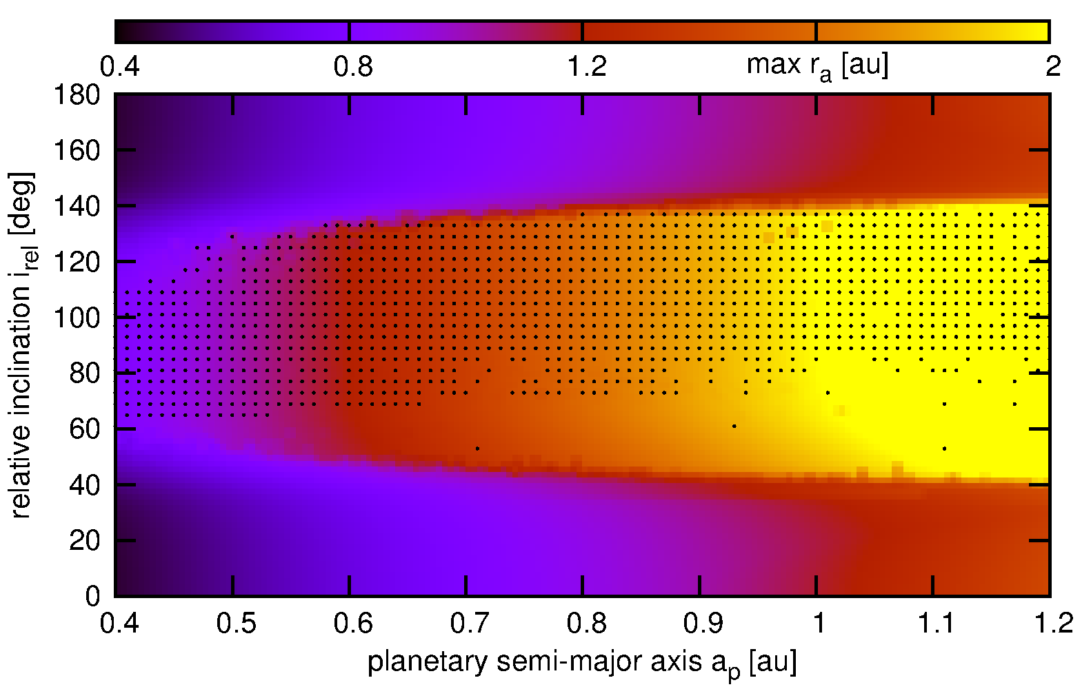
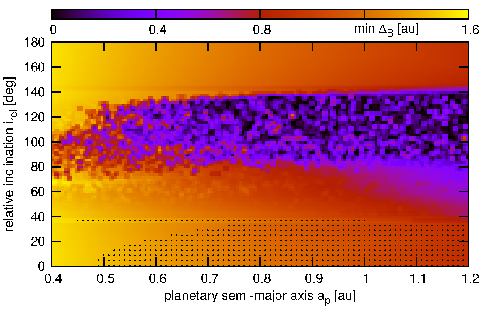
Figure 4: The orbital evolution of the secular system in terms of the octupole–level expansion w.r.t. $\alpha=a_{\mbox{\scriptsize p}}/a_{\mbox{\scriptsize bin}}$. The left column is for the nominal secondary $m_{\mbox{\scriptsize B}}=$532 m${}_{\mbox{\scriptsize Jup}}$, the right column is for the secondary mass $m_{\mbox{\scriptsize B}}=$14 m${}_{\mbox{\scriptsize Jup}}$. The initial geometric elements are fixed to keep $\Delta\varpi\equiv\varpi_{\mbox{\scriptsize p}}-\varpi_{\mbox{\scriptsize S}}=0^{\circ}$ in the Laplace reference frame (aligned orbits). The top row is for the maximum eccentricity of the planet, the middle row is for the maximum of the apocenter distance of the planet and the bottom row is the minimum distance of the planet from the perturber. Dotted areas mark librations of $\Delta\varpi$ in the top panels, collisional orbits with the primary in the middle panels, and librations of $\Delta\varpi$ in the bottom panels.

3 Re-analysis of the RV data

It is well known that the RV measurements errors originate from the formal errors $\sigma_{\mbox{\scriptsize m}}$ of the Doppler method, systematic uncertainties due to instrumental instabilities, as well as from internal chromospheric variability $\sigma_{\mbox{\scriptsize jitter}}$ of the parent star. The later error is difficult to quantify particularly for young or active stars. In the recent literature, it is common to derive astrophysical estimates of the jitter $\sigma_{\mbox{\scriptsize jitter}}$ (Wright, 2005). Joint error of the measurements are obtained by adding both uncertainties in quadrature for each data point. Recently, Baluev (2009) has shown how to estimate $\sigma_{\mbox{\scriptsize jitter}}$ as an additional free parameter of the fit model. Here, we follow the earlier, somehow more traditional approach. In this work, we computed the best-fit models after rescaling the measurement errors in (Ramm et al., 2009) by two values of $\sigma_{\mbox{\scriptsize jitter}}$. For the first class of models, we choose $\sigma_{\mbox{\scriptsize jitter}}=5$ $\mbox{ms}^{-1}$, which is relatively small value, exhibited by quiet, non-active stars, and likely too conservative in our case. The second family of solutions was obtained for $\sigma_{\mbox{\scriptsize jitter}}=20$ $\mbox{ms}^{-1}$. This value of jitter uncertainty seems better justified recalling large residuals of the Keplerian model in the discovery paper of a similar magnitude ($\sim 20$ $\mbox{ms}^{-1}$). Using these RV data, we optimized different 2-planet models. The astrometric data gathered by Hipparchos were used indirectly, by fixing the nodal line and inclination of the binary orbit close to the combined astrometric and radial velocity solution in (Ramm et al., 2009).

3.1 Keplerian (kinematic) model of the RV

In the first fitting experiment, we search for the best-fit Keplerian, non-interacting orbits. Hence, we basically follow the discovery paper. The best-fit configurations of $\nu$ Oct system were found after extensive search performed with the hybrid optimization algorithm (see Goździewski et al., 2008, and references therein). It consists on two stages: a quasi-global Genetic Algorithm which provides many reasonably precise models, and the Levenberg-Marquardt (LM) method which is used to refine these solutions.

The results are illustrated in Fig. 5, in the form of ${(\chi^{2}_{\nu})^{1/2}}$ parameter scans illustrated in the orbital period $P_{\mbox{\scriptsize p}}$ – eccentricity $e_{\mbox{\scriptsize p}}$ plane of the planet. Curiously, for both selected jitter uncertainties, we found a well defined secondary minimum for $P_{\mbox{\scriptsize p}}\sim 900$ days and $e_{\mbox{\scriptsize p}}\sim 0.3$, besides the best-fit model reported by Ramm et al. (2009) with $P_{\mbox{\scriptsize p}}\sim 420$ days and $e_{\mbox{\scriptsize p}}\sim 0.1$. A choice of the jitter uncertainty may lead to significant changes of the ${(\chi^{2}_{\nu})^{1/2}}$ shape and alters formal errors of the best-fit parameters. This effect is important for fixing parameter bounds in dynamical studies made after the best-fit models are found. Moreover, because the secondary best-fit configuration has the planetary period comparable with the binary period, its interpretation in terms of the osculating elements becomes even more questionable than in the case of the primary minimum of ${(\chi^{2}_{\nu})^{1/2}}$, as underlined in the introduction. The secondary solution might correspond to 1:1 MMR which obviously would require a more general $N$-body model of the RV which takes into account all mutual interactions between the bodies in the system (Laughlin & Chambers, 2001).

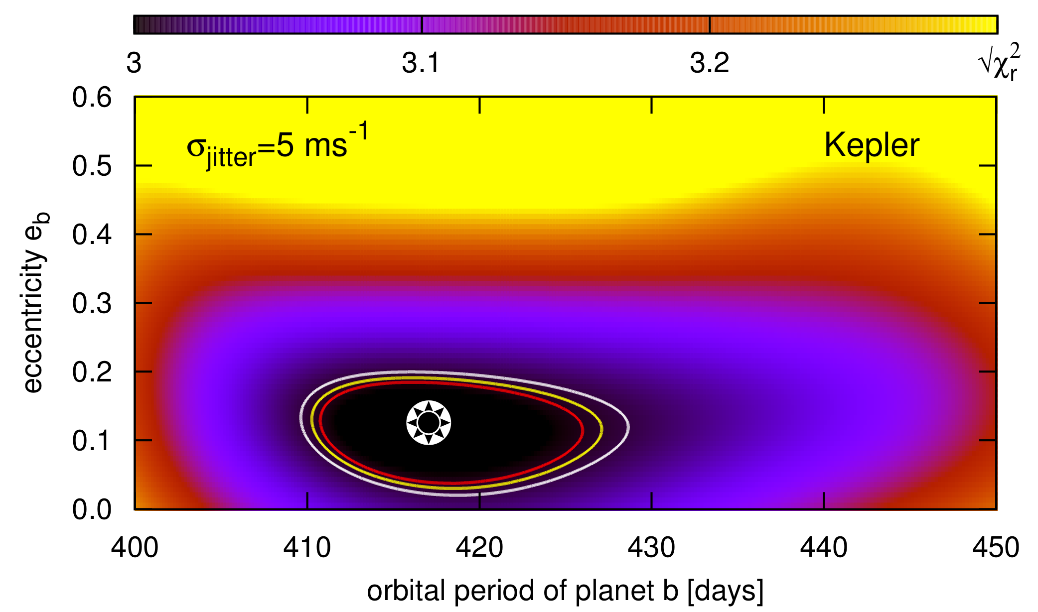
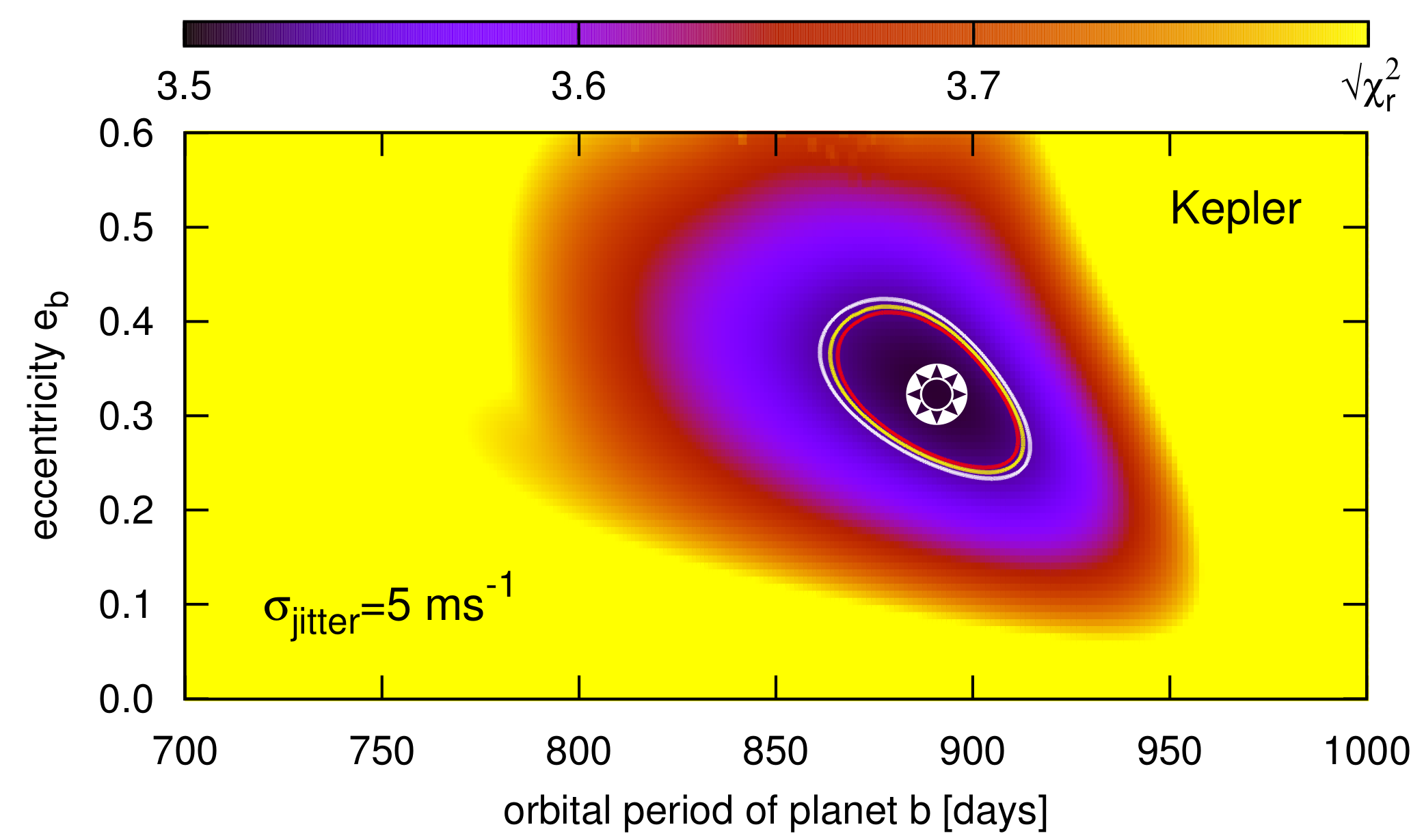
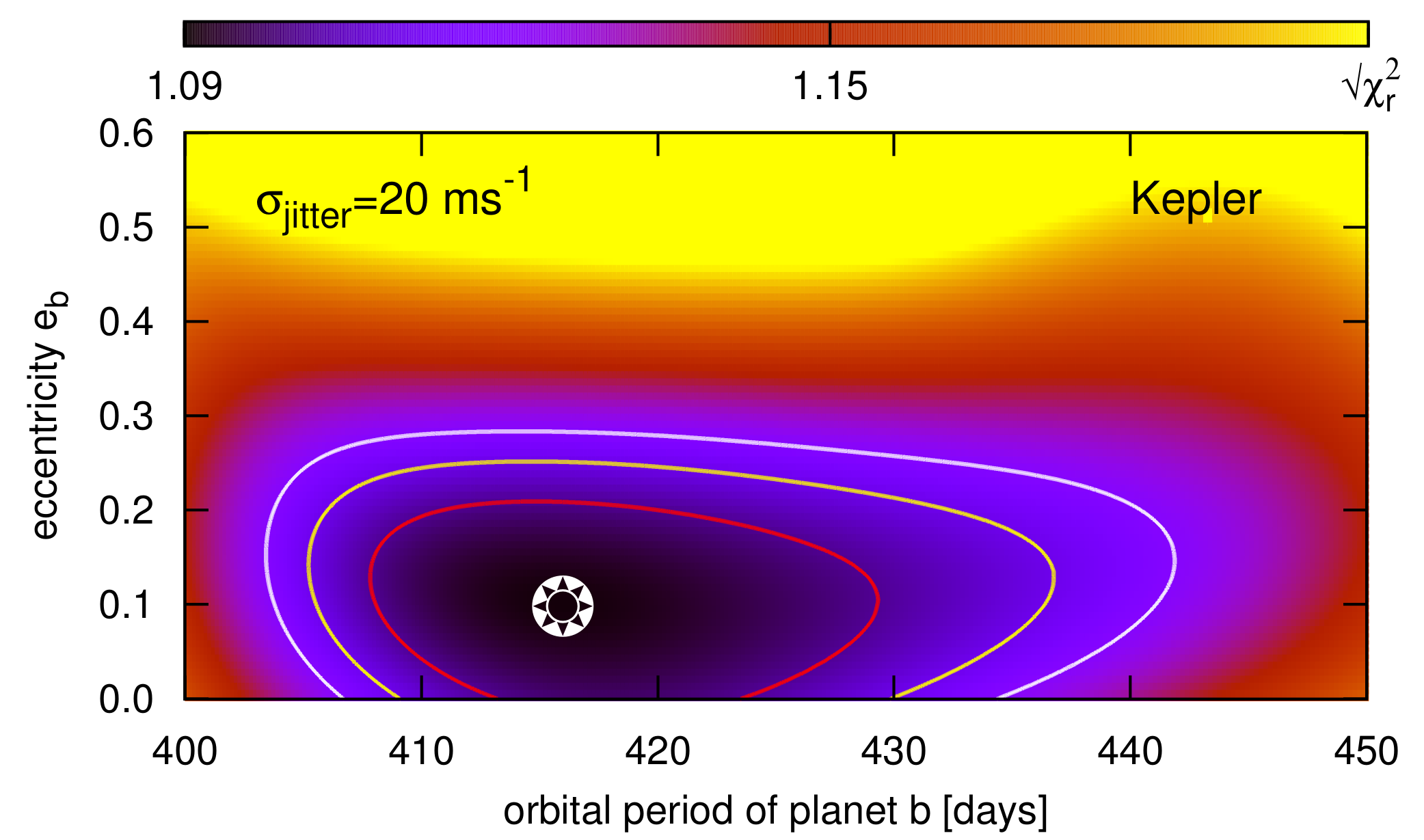
Figure 5: The topology of ${(\chi^{2}_{\nu})^{1/2}}$ in the orbital period–eccentricity plane of the putative planet for two values of the jitter uncertainty. The top row is for $\sigma_{\mbox{\scriptsize jitter}}=5$ $\mbox{ms}^{-1}$, the bottom plot is for $\sigma_{\mbox{\scriptsize jitter}}=20$ $\mbox{ms}^{-1}$. Smooth, coloured curves are for formal 1,2,3$\sigma$ levels of the best-fit model marked with a star symbol.

3.2 The self-consistent, Newtonian model of the RV

As we have shown above, the Keplerian model of $\nu$ Oct data is non-unique, permitting two different solutions. It is also well known that it is independent on orbital inclinations and true masses. Due to the massive secondary, the RV-model including mutual interactions between all system components might constrain these parameters, in spite of a narrow observational window, like in other interacting extrasolar planetary systems (Laughlin & Chambers, 2001). Hence, in the second fitting experiment, to compute the RVs of the primary, we integrated the $N$-body equations of motion. In this model, the primary mass $m_{\mbox{\scriptsize bin}}$, its semi–major axis $a_{\mbox{\scriptsize bin}}$, eccentricity $e_{\mbox{\scriptsize bin}}$ of the binary, pericenter argument $\omega_{\mbox{\scriptsize bin}}$, inclination $i_{\mbox{\scriptsize bin}}$ and the initial mean anomaly ${\cal M}_{\mbox{\scriptsize bin}}$ of the binary were allowed to vary within the formal $3\sigma$ error bounds, in accord with the combined RV and astrometric solution in Ramm et al. (2009). The nodal longitude of the binary was fixed, $\Omega_{\mbox{\scriptsize bin}}=87^{\circ}$. The formal error of this element is irrelevant for the dynamics of the system, because selecting the nodal line of the binary corresponds to a choice of the $x$–axis of the reference frame. The planet mass $m_{\mbox{\scriptsize p}}$, its inclination $i_{\mbox{\scriptsize p}}$, the nodal longitude $\Omega_{\mbox{\scriptsize p}}$ and the remaining orbital elements with the RV offset were added to the set of 14 free parameters of the fit model. The uncertainties of the measurements in (Ramm et al., 2009) were rescaled in quadrature, as in the Keplerian model, to account for the intrinsic stellar RV variability.

Similar to the Keplerian model, we explored the parameter space with the hybrid algorithm. After an extensive search, we selected the best-fit $N$-body configuration. Then we reconstructed the shape of ${(\chi^{2}_{\nu})^{1/2}}$ around this nominal solution in 2-dimensional planes of various orbital elements. Its parameters derived with $\sigma_{\mbox{\scriptsize jitter}}=5$ $\mbox{ms}^{-1}$are given in Table 1 (Fit I). The RV data in Ramm et al. (2009) consist of many “clumps” of measurements done during one night, which cover less than 0.1 day. Such data points were binned, and the resulting data set consists of 91 measurements. This step was helpful to improve the CPU-efficiency, due to necessity of computing numerical derivatives in the LM algorithm. We examined that ${(\chi^{2}_{\nu})^{1/2}}$-scans can be reproduced with the full, original data set. Obtaining a smooth shapes of ${(\chi^{2}_{\nu})^{1/2}}$ for non-binned data is difficult, due to numerical errors introduced by the numerical derivatives.

The $(a_{\mbox{\scriptsize p}},e_{\mbox{\scriptsize p}})$–plane (Fig. 6, the top-lef panel) makes it possible to compare the topology of ${(\chi^{2}_{\nu})^{1/2}}$ in both RV-models. Clearly, the best-fit Newtonian configuration is qualitatively different from the Keplerian models found in the previous section which confirms our earlier predictions. The planet eccentricity may be as large as $\sim 0.45$. The low estimate of $\sigma_{\mbox{\scriptsize jitter}}\sim 5$ $\mbox{ms}^{-1}$ implies two, statistically distinct close minima of ${(\chi^{2}_{\nu})^{1/2}}$, for $a_{\mbox{\scriptsize p}}\sim 1.25$ au, and better model for $a_{\mbox{\scriptsize p}}\sim 1.4$ au. These minima are resolved at the formal $2\sigma$–error level of ${(\chi^{2}_{\nu})^{1/2}}$. If the jitter estimate is larger, likely much more realistic, only one solution persist (see Fig. 7, the top left panel). In this case, the formal $1\sigma$ error of $a_{\mbox{\scriptsize p}}$ spans almost $0.3$ au.

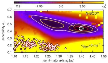
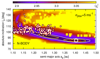
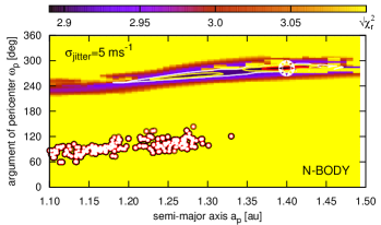
Figure 6: The shape of ${(\chi^{2}_{\nu})^{1/2}}$ in different orbital planes of the planet computed in terms of the self-consistent $N$-body model of the RV. Jitter uncertainty is $\sigma_{\mbox{\scriptsize jitter}}\sim 5$ $\mbox{ms}^{-1}$. The RV data in (Ramm et al. 2012) are binned (see the text for details). Quality of solutions is color coded. Smooth, coloured curves are for formal 1,2,3$\sigma$ confidence levels of the best-fit model marked with an asterisk. Its elements recomputed on the original data set are given in Table 1 (Fit I). Smaller, filled circles mark stable solutions found with through the GAMP search, and projected onto planes of orbital osculating elements at the epoch of the first observation in (Ramm et al. 2009). An rms of these solutions is less than 28 $\mbox{ms}^{-1}$.

Even more interesting results are illustrated in the next panels of Figs. 6 and 7 showing scans of ${(\chi^{2}_{\nu})^{1/2}}$ in the semi-major axis–inclination, —longitude of the node and —the pericenter argument planes, respectively. ${(\chi^{2}_{\nu})^{1/2}}$ scans computed for $\sigma_{\mbox{\scriptsize jitter}}\sim 5$ $\mbox{ms}^{-1}$ reveal two minima seen in Fig. 6. Such scans for $\sigma_{\mbox{\scriptsize jitter}}\sim 20$ $\mbox{ms}^{-1}$ (Fig. 7) illustrate that the global minimum around $(a_{\mbox{\scriptsize p}}=1.40$ au, $e_{\mbox{\scriptsize p}}=0.45)$ is well defined in all planes of angular elements. This means that even a narrow observational window, covering roughly 2 planetary periods, makes it possible to estimate all angles of the orbit due to strong mutual interactions in the system. This experiment is a convincing illustration that the Keplerian, kinematic model of $\nu$ Oct is questionable because it looses information of the node and inclination of the orbit. A proper estimate of the jitter uncertainty is vital to derive true errors of the best-fit model. We found that the best-fit model (Fit I in Table 1) tends towards the lower bound of inclination (69^∘), with simultaneous increase of the secondary mass. This effect appears because the inclination of the binary cannot be constrained by the RV data alone. Likely, dynamically consistent $N$–body model of the $\nu$ Oct system should also incorporate the Hipparchos astrometry, which would be helpful to fix the orbit of the binary fully consistent with all data and the three-body model. We postpone this analysis to another work.

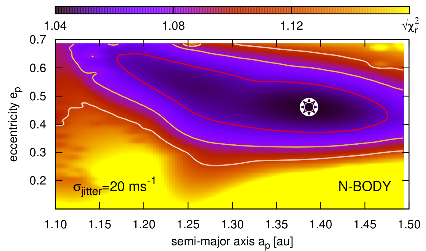
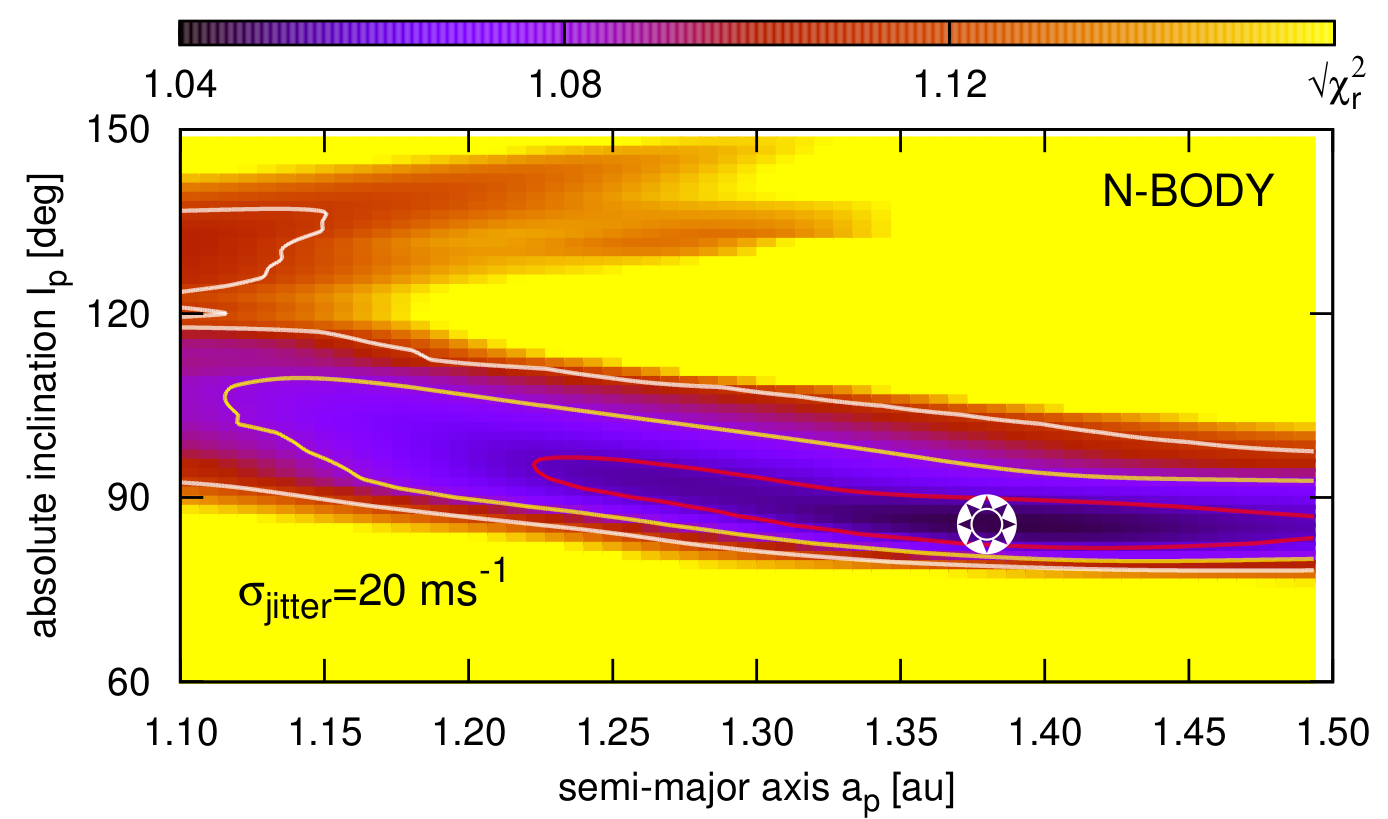
Figure 7: The shape of ${(\chi^{2}_{\nu})^{1/2}}$ in terms of the Newtonian model illustrated in different orbital parameter planes, as derived for jitter uncertainty $\sigma_{\mbox{\scriptsize jitter}}\sim 20$ $\mbox{ms}^{-1}$. Quality of solutions is color coded. The best-fit configuration is marked with an asterisk.

3.3 Newtonian model with stability constraints

Unfortunately, the best-fit Newtonian model (Fit I in Table 1) found through the hybrid search leads to strongly unstable system. Due to relatively large parameter error, stable configurations might be still possible in its neighborhood. Hence, we conducted an additional, extensive search for stable models imposing stability constraints (GAMP algorithm, Goździewski et al., 2008). In this approach, unstable models are “penalized” by an artificial, large value of ${(\chi^{2}_{\nu})^{1/2}}$ (or an rms) and are excluded during the optimization. The results are shown in Fig. 6. Stable fits exhibit systematically larger ${(\chi^{2}_{\nu})^{1/2}}$ than the best–fit model in Table 1. To illustrate the statistics of such configurations, we over-plotted solutions with an rms $<28$ $\mbox{ms}^{-1}$ (white, filled circles) at the top of selected parameter scans of ${(\chi^{2}_{\nu})^{1/2}}$ (Fig. 6). Let us note that stable models have the MEGNO signature $\sim 2$ for $2000~{}P_{\mbox{\scriptsize bin}}$. This relatively short integration period requires an acceptable CPU-overhead from the hybrid algorithm, still providing at least 10-100 longer Lagrange stability time. Such solutions should survive for $10^{4}$–$10^{5}$ $P_{\mbox{\scriptsize bin}}$ or even longer integration time (Cincotta et al., 2003). The statistics in Fig. 6 reveals that the formal best-fit configurations in terms of “pure” $N$-body model are systematically shifted by more than $3\sigma$ from the best-fit GAMP (stable) models. This regards all orbital parameters, and in particular, the eccentricity and the argument of pericenter. This large discrepancy may indicate that the 2-planet model is in fact not proper, and should be rejected at all or modified. Curiously, we found stable solutions only as retrograde orbits, actually in accord with the original hypothesis in (Eberle & Cuntz, 2010) and later investigated by Quarles et al. (2012). This is illustrated in Fig. 8 showing that differences of the longitudes of periastrons and of the nodal longitudes are well bounded around $180^{\circ}$, resulting in apsidal lines of the orbits which are significantly anti-aligned (the left panel). Large relative inclinations of these stable solutions (the right panel) mean retrograde orbits in the range of $a_{\mbox{\scriptsize p}}\sim$ around 1.2 au.

To compare the quality of these two families of models in terms of an rms, the RV residuals of two selected best–fit models are displayed in Fig. 9: the first one derived without stability constraints (Fit I in Tab. 1, the left panel), and an low rms stable model ( the right panel, Fit II in Table 1). In both cases, the residuals exhibit a large magnitude of $\sim 120$–$150$ $\mbox{ms}^{-1}$, comparable with the semi-amplitude of the RV signal $\sim 100$ $\mbox{ms}^{-1}$ due to the putative planet itself. In this sense, stable solutions might be still acceptable, although their rms is significantly larger from the rms of the formal best-fit model configuration. A large variability of the RV residuals cannot be well explained by the 1-planet model. This may indicate strong stellar activity mimicking planetary signal.

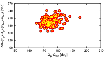
Figure 8: The statistics of stable best-fit models (see Fig. 6) projected onto selected planes of the orbital osculating elements at the epoch of the first observation in (Ramm et al. 2009). These fits are gathered in the hybrid GAMP search (see the text for details). An rms of these solutions is less than 28 $\mbox{ms}^{-1}$.

Table 1: The best-fit astro-centric, osculating Keplerian elements of the $\nu$ Octantis planetary system at the first epoch in (Ramm et al. 2009). The RV data errors in the discovery paper are rescaled with the jitter uncertainty $\sigma_{\mbox{\scriptsize jitter}}=5$ $\mbox{ms}^{-1}$in quadrature. The nodal longitude of the binary orbit is fixed to 87 deg. Mass of the primary $\nu$ Oct A is 1.4 $m_{\odot}$. Parameters of stable solutions (Fits II and III) are quoted with many digits making it possible to demonstrate stability of these solutions in very narrow stable zones. Formal errors of these fits can be estimated as equal or similar to the uncertainties quoted for parameters of formal, $N$-body Fit I.

	Fit I ($N$-body, unstable)		Fit II (GAMP, stable)		Fit III (GAMP, stable)
Parameter	planet $\nu$ OctAb	$\nu$ Oct B	planet $\nu$ OctAb	$\nu$ Oct B	planet $\nu$ OctAb	$\nu$ Oct B
mass $m$ [m${}_{\mbox{\scriptsize Jup}}$]	3.54 $\pm$ 0.07	572 $\pm$ 15	1.92596	560.62366	2.135457	559.2707
semi-major axis $a$ [AU]	1.41 $\pm$ 0.02	2.533 $\pm$ 0.005	1.16365	2.52813	1.160281	2.526478
eccentricity $e$	0.40 $\pm$ 0.01	0.2331 $\pm$ 0.0006	0.13139	0.23881	0.247587	0.238713
inclination $i$ [deg]	84.9 $\pm$ 2.2	69.0 $\pm$ 3.3	110.21102	71.28090	102.4152	71.681
longitude of the node $\Omega$ [deg]	289.2 $\pm$ 4.2	87.0 (fixed)	262.29811	87.0 (fixed)	260.0224	87.0 (fixed)
argument of pericenter $\omega$ [deg]	340.6 $\pm$ 2.6	75.0 $\pm$ 0.1	127.26299	74.59137	88.86501	74.85992
mean anomaly ${\cal M}(t_{0})$ [deg]	289.2 $\pm$ 4.2	339.5 $\pm$ 0.l	133.16327	339.762973	165.3685	339.5231
${(\chi^{2}_{\nu})^{1/2}}$	2.79		3.47		3.44
RV offset $V_{0}$ [m s-1]	-6417 $\pm$ 1		-6473.682		-6475.317
rms [m s-1]	19.9		25.2		24.8

3.4 Stability of the best-fit GAMP configurations

To illustrate the dynamical neighborhood of the best–fit GAMP models, we selected two examples of low rms configurations. Their osculating elements at the epoch of the first observation in (Ramm et al., 2009) are given in Table 1 (Fits II and III). Many digits are quoted, to reproduce elements of these fit possibly exactly, to make it possible to reproduce their stable evolution due to complex and chaotic neighborhoods. The formal errors may be estimated graphically in Fig. 6 or interpreted as uncertainties of the formal Fit I. The primary mass is fixed as equal to 1.4 M_⊙. An rms of this solution is $\sim 25$ $\mbox{ms}^{-1}$.

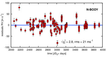
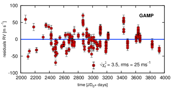
Figure 9: Residuals to representative self-consistent, Newtonian best-fit models illustrated in Fig. 8. The left panel is for the formal, mathematical $N$-body solution (Fit I in Table 1). The right panel is for a stable, low-rms GAMP–derived model (Fit II in Table 1).

The top-left panel of Fig. 10 illustrates the MEGNO dynamical map in the $(a_{\mbox{\scriptsize p}},i_{\mbox{\scriptsize p}})$–plane computed for Fit II (see Tab.1). This map shows a global view of the phase space. Note that inclination $i_{\mbox{\scriptsize p}}$ is absolute w.r.t. the astrometric frame, in which the binary inclination is bounded around $i_{\mbox{\scriptsize bin}}\sim 71^{\circ}$. This figure reveals that the phase space is mostly strongly chaotic. The best–fit configuration is found in a narrow stability island close to the 7:2 MMR. For a reference, other significant MMRs are labeled. A close-up of this map shown in the top–right panel of Fig. 10 reveals an extremely complex structure of this regular island. It spans a tiny region covering $\Delta a_{\mbox{\scriptsize p}}\sim 0.02$ au and $\Delta i_{\mbox{\scriptsize p}}\sim 20^{\circ}$. In this small island, the phase space has again a sophisticated, fractal-like structure of the Arnold web.

The integration time used to derive the global dynamical map in the left panel of Fig. 10 is $1\times 10^{4}P_{\mbox{\scriptsize bin}}$. Subsequent close-ups shown in Fig. 10 were integrated for $2\times 10^{4}P_{\mbox{\scriptsize bin}}$ up to $1\times 10^{5}P_{\mbox{\scriptsize bin}}$ per each point, depending on the magnification factor. To detect weak MMRs and their sub-resonances, such long integration times are indispensable. The resolution of these maps is $1440\times 900$ pixels. Calculations were performed with the help of the Mechanic installed on the UV SGI supercomputer chimera of the Poznań Supercomputing Centre (Poland).

We computed a similar set of dynamical maps for another stable model, with larger eccentricity (Fit III in Table 1). The results are illustrated in Fig. 11. The top left panel illustrates the dynamical map in the ($a_{\mbox{\scriptsize p}},e_{\mbox{\scriptsize p}}$)–plane, showing a narrow stable island of this solution, the rest of plots are for the ($a_{\mbox{\scriptsize p}},i_{\mbox{\scriptsize p}}$)–plane and its close-ups.

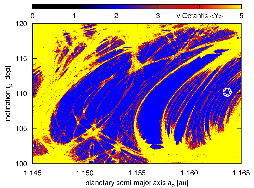
Figure 10: Dynamical MEGNO maps of a stable model found in the GAMP search illustrated in the ($a_{\mbox{\scriptsize p}},i_{\mbox{\scriptsize p}})$–plane. The top left panel is for the global view of the phase space, the top right map is for stability island of the solution. Subsequent maps are for close-ups of the neighborhood of the best–fit solution. Osculating, astrocentric elements of the planet and the secondary are given in Table 1 (Fit II). The nominal elements are marked with the star symbol. The raw resolution of the maps is 1440$\times$900 data points.

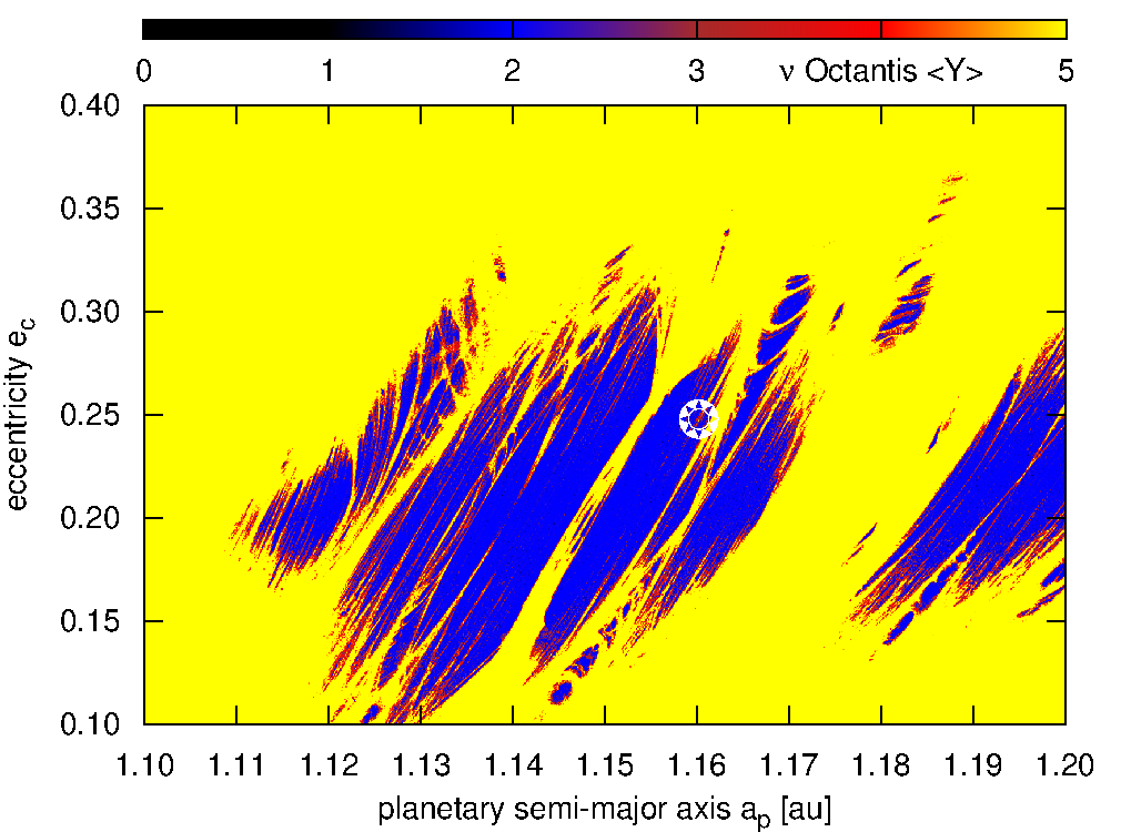
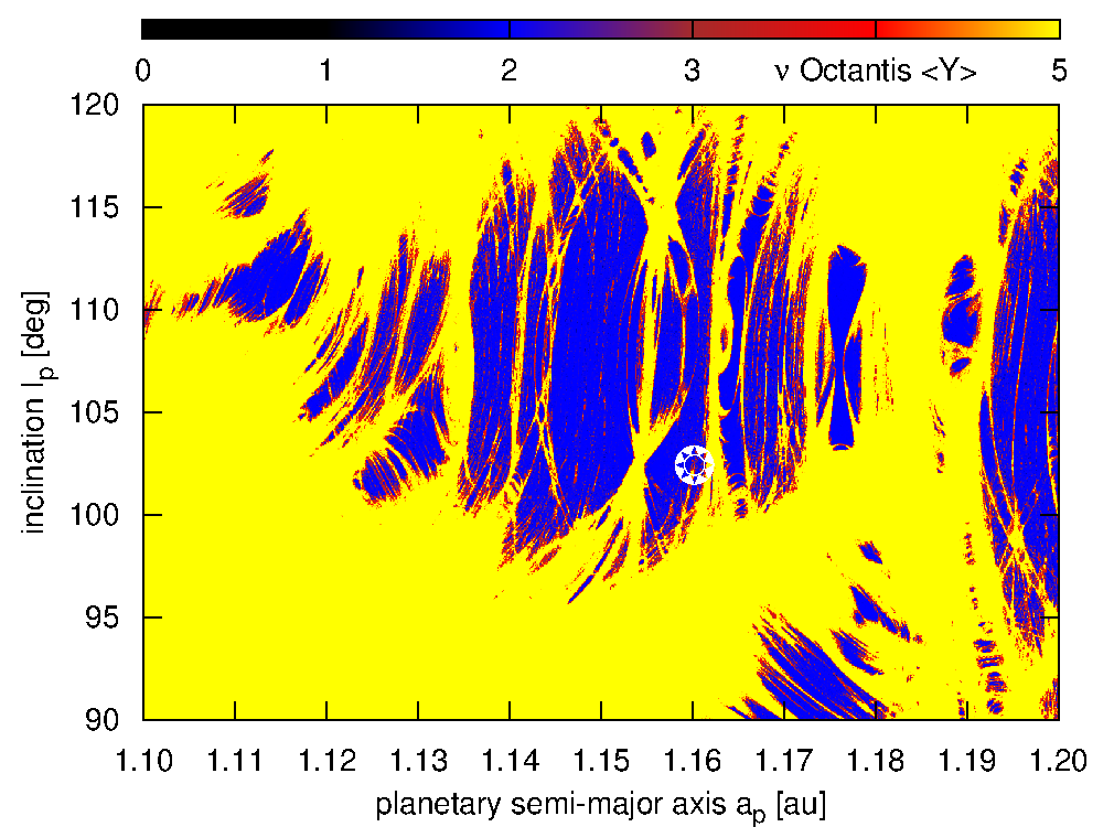
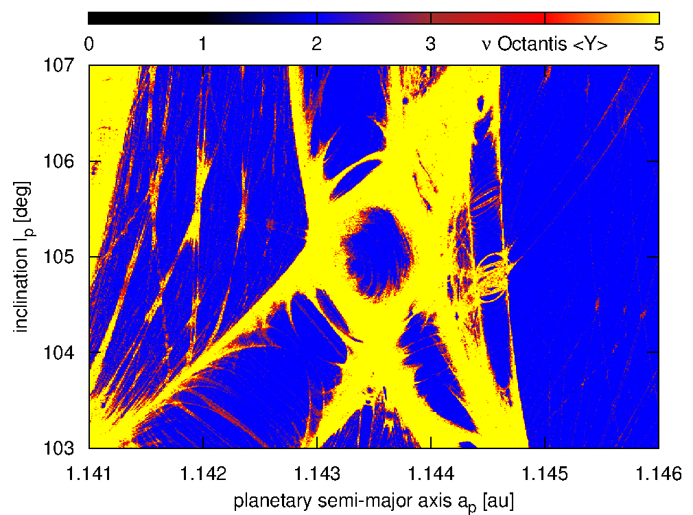
Figure 11: Dynamical MEGNO maps of a stable model with moderate eccentricity of the planet as found in the GAMP search illustrated in the ($a_{\mbox{\scriptsize p}},e_{\mbox{\scriptsize p}})$ and ($a_{\mbox{\scriptsize p}},i_{\mbox{\scriptsize p}})$–plane. Bottom panels show close-ups of the top right panel. Osculating, astrocentric elements of the planet and the secondary are given in Table 1 (Fit III). The nominal elements are marked with the star symbol. The raw resolution of the maps is 1440$\times$900 data points.

To reveal the Arnold web in more detail, we computed a number of close-ups shown in panels of Figs. 10–12. These maps reveal many weak sub-resonances, which form a regular net present at any magnification level. These structures are particularly well seen in the bottom-right panel of Fig. 12. They closely resemble the Arnold web of the model Hamiltonian (Froeschlé et al., 2000). Likely, it has been never illustrated with such a sharpness and details. We also tested other solutions from the GAMP–derived set. The results are similar. The best–fit models which obey reasonably well the observational constrains are confined to only narrow stability islands.

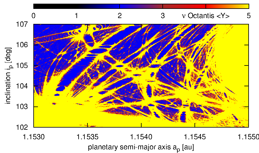
Figure 12: A close-up of a stability island of the best-fit, stable GAMP Fit II (Table 1) illustrated in Fig. 10. The resolution is $1440\times 900$ pixels. The integration time per pixel is $3\times 10^{5}$ orbital periods of the binary.

4 Conclusions

In this work, we aim to improve the original Keplerian models of the $\nu$ Oct system. We re-analysed the RV observations in (Ramm et al., 2009). The results confirm our predictions on a significance of the mutual interactions between the secondary and the putative planet. These interactions are so strong that – if the planet is real – it might be possible to derive the orientation of the orbit with respect to the binary, and its true mass, in spite of a narrow observational window spanning less than 2 orbital periods.

We confirm that stable retrograde solutions in the $\nu$ Oct planetary system are possible as proposed in (Eberle & Cuntz, 2010; Quarles et al., 2012). However, the observational constrains imply such orbits with apsidal lines initially anti-aligned with the apses of the binary. The long-term stable solutions may be found only in relatively small islands of regular, quasi-periodic motions exhibiting a complex structure of the Arnold web. Stable models must be significantly shifted in the parameter space from the $N$-body and Keplerian best-fit models. It means that the 2-planet, S-type configuration is most likely inadequate to fit the available data set. It remains highly uncertain how a massive, Jovian planet could be trapped in such tiny stable regions, or how it might form in globally unstable dynamical environment. The observational RV signal is very noisy, and the best-fit models reveal a large scatter of residuals having amplitude comparable with the RV signal itself. These arguments make the hypothesis of Jovian planet in orbit around $\nu$ Oct A questionable. Actually, this in accord with the doubts raised in the discovery paper (Ramm et al., 2009). New observations are required to confirm or withdraw that explanation of the observed RV residual signal, and to search for alternate dynamical models of the detected variability.

An efficient analysis of the observations of extrasolar planetary systems involves not only different observational techniques and data sources, but also orbital optimization algorithms, combined with analytical and numerical stability studies. In this work, we propose and apply our new MPI-based task management system Mechanic to perform high-resolution dynamical mapping of the phase space. This framework is devoted to numerical analysis of large sets of initial conditions, like the long-term integrations of the equations of motion. We work on other applications, like quasi-global optimization with the Genetic Algorithms of different observational models of the extrasolar planetary systems. The Mechanic code with detailed technical documentation and sample modules is freely available at the project website (Słonina & Goździewski, 2012).

5 Acknowledgments

We thank the anonymous referees for their reviews that improved this paper. This work is supported by the Polish Ministry of Science and Higher Education through grant N/N203/402739. Computations were conducted thanks to the POWIEW project of the European Regional Development Fund in Innovative Economy Programme POIG.02.03.00-00-018/08.

References

- Adams & Laughlin (2003) Adams F. C., Laughlin G., 2003, Icarus, 163, 290
- Alden (1939) Alden H. L., 1939, AJ, 48, 81
- Baluev (2009) Baluev R. V., 2009, MNRAS, 393, 969
- Baluev (2011) Baluev R. V., 2011, Celestial Mechanics and Dynamical Astronomy, 111, 235
- Beaugé et al. (2012) Beaugé C., Ferraz-Mello S., Michtchenko T. A., 2012, Research in Astronomy and Astrophysics, 12, 1044
- Chambers (1999) Chambers J. E., 1999, MNRAS, 304, 793
- Cincotta et al. (2003) Cincotta P. M., Giordano C. M., Simó C., 2003, Physica D Nonlinear Phenomena, 182, 151
- Colacevich (1935) Colacevich A., 1935, PASP, 47, 87
- Dvorak (1984) Dvorak R., 1984, Celestial Mechanics, 34, 369
- Eberle & Cuntz (2010) Eberle J., Cuntz M., 2010, ApJL, 721, L168
- Froeschlé et al. (2000) Froeschlé C., Guzzo M., Lega E., 2000, Science, 289, 2108
- Goździewski et al. (2008) Goździewski K., Breiter S., Borczyk W., 2008, MNRAS, 383, 989
- Guzzo (2005) Guzzo M., 2005, Icarus, 174, 273
- Guzzo (2006) Guzzo M., 2006, Icarus, 181, 475
- Hairer et al. (1993) Hairer E., Norsett S. P., Wanner G., 1993, Solving Ordinary Differential Equations I. Nonstiff Problems. Springer Verlag
- Holman & Wiegert (1999) Holman M. J., Wiegert P. A., 1999, AJ, 117, 621
- Jefferys (1974) Jefferys W. H., 1974, AJ, 79, 710
- Kley (2010) Kley W., 2010, in K. Go zdziewski, A. Niedzielski, & J. Schneider ed., EAS Publications Series Vol. 42 of EAS Publications Series, The formation of massive planets in binary star systems. pp 227–238
- Kozai (1962) Kozai Y., 1962, AJ, 67, 591
- Laughlin & Chambers (2001) Laughlin G., Chambers J. E., 2001, ApJL, 551, L109
- Migaszewski & Goździewski (2011) Migaszewski C., Goździewski K., 2011, MNRAS, 411, 565
- Migaszewski et al. (2012) Migaszewski C., Słonina M., Goździewski K., 2012, MNRAS, 427, 770
- Morais & Correia (2012) Morais M. H. M., Correia A. C. M., 2012, MNRAS, 419, 3447
- Morais & Giuppone (2012) Morais M. H. M., Giuppone C. A., 2012, MNRAS, 424, 52
- Mudryk & Wu (2006) Mudryk L. R., Wu Y., 2006, ApJ, 639, 423
- Quarles et al. (2012) Quarles B., Cuntz M., Musielak Z. E., 2012, MNRAS, 421, 2930
- Ramm et al. (2009) Ramm D. J., Pourbaix D., Hearnshaw J. B., Komonjinda S., 2009, MNRAS, 394, 1695
- Słonina & Goździewski (2012) Słonina M., Goździewski K., , 2012, The Mechanic User Guide, http://git.astri.umk.pl
- Słonina et al. (2012) Słonina M., Goździewski K., Migaszewski C., 2012, in Arenou F., Hestroffer D., eds, Proceedings of the workshop ”Orbital Couples: Pas de Deux in the Solar System and the Milky Way”. Held at the Observatoire de Paris, 10-12 October 2011. Editors: F. Arenou, D. Hestroffer. ISBN 2-910015-64-5, p. 125-129 Mechanic: a new numerical MPI framework for the dynamical astronomy. pp 125–129
- Szebehely (1967) Szebehely V., 1967, Theory of orbits. The restricted problem of three bodies
- Wisdom (1983) Wisdom J., 1983, Icarus, 56, 51
- Wright (2005) Wright J. T., 2005, PASP, 117, 657