Scaling ansatz, four zero Yukawa textures and large $\theta_{13}$

Abstract

We investigate ’Scaling ansatz’ in the neutrino sector within the framework of type I seesaw mechanism with diagonal charged lepton and right handed Majorana neutrino mass matrices ($M_{R}$). We also assume four zero texture of Dirac neutrino mass matrices ($m_{D}$) which severely constrain the phenomenological outcomes of such scheme. Scaling ansatz and the present neutrino data allow only Six such matrices out of 126 four zero Yukawa matrices. In this scheme, in order to generate large $\theta_{13}$ we break scaling ansatz in $m_{D}$ through a perturbation parameter and we also show our breaking scheme is radiatively stable. We further investigate CP violation and baryogenesis via leptogenesis in those surviving textures.

I Introduction

Neutrino physics is now playing a pivotal role to probe physics beyond the Standard Model. Confirmation of tiny neutrino masses as well as nonzero mixing angles have thrown light on the structure of the leptonic sector. In the quest towards understanding of a viable texture of neutrino mass matrix popular paradigm is to advocate flavor symmetries, directly associated with some gauge group. On the other hand, there are some other ansatzs which also give rise to interesting phenomenological consequences, although their origin from a symmetry discrete or continuous are yet to be established at the present moment.
In the present work we bring together two ideas to explore the neutrino phenomenology, particularly, to generate large $\theta_{13}$ Gluza -ema as reported by recent experiments minos1 -last as well as CP violation and baryogenesis via leptogenesis. In this scheme we consider a) Scaling ansatzsc1 -sc3 , b) Four zero texture 4zero1 -4zero4 of Dirac neutrino matrix $(m_{D})$, within the framework of type I seesaw mechanism denoted as

$$m_{\nu}=-m_{D}M_{R}^{-1}m_{D}^{T}$$ (1)

where $M_{R}$ is a $3\times 3$ right chiral neutrino mass matrix and we consider the basis in which charged lepton and $M_{R}$ are flavor diagonal. Scaling ansatz sc1 -sc3 posses a distinctive feature that the texture is invariant under renormalisation group evolution unlike other symmetries such as $\mu-\tau$ symmetry. Basically, the ansatz correlates the elements of neutrino mass matrix through a scale factor and it can be implemented in different ways. Although the theoretical origin of such ansatz is not yet well known, however, this ansatz can be approximated as $S_{2L}$ symmetry (i.e $\mu-\tau$ symmetry in the left handed neutrinos) with the value of the scale factor unity. Furthermore, it leads to inverted hierarchy of neutrino mass with $m_{3}$ = 0, and $\theta_{13}$ = 0. Thus, it is obvious to break such ansatz in order to generate nonzero $\theta_{13}$. The other assumption that occurrence of four zeroes in $m_{D}$ gives rise to a more constrained feature that the phases contributing to the high scale CP violation required for leptogenesis (basically the phases of $m_{D}m_{D}^{\dagger}$ matrix) are determined in terms of the low energy CP violating phases ( i.e phases of $m_{\nu}$). We divide all the $9_{{C}_{4}}=126$ four zero textures in the following Classes : i) det($m_{D}$)= 0 and no generation decouples: $27$ textures ii) det($m_{D}$) $\neq$ 0 and no generation decouples: $72$ textures. iii)det($m_{D}$)= 0 and one generation decouples: $18$ textures iv) det($m_{D}$) $\neq 0$ and one generation decouples: $9$ textures The textures belong to Class (ii) are already studied extensively 4zero1 -4zero4 . Class (iii) and (iv) are incompatible with the neutrino experimental result. The remaining Class, Class (i), which is yet to be explored, posses one zero eigenvalue which is still allowed by the present experiments. The interesting point is to note that if we insert scaling ansatz to all four zero textures and consider those textures in which four zero remain four zero and no generation decouples, we see that the survived textures are only from Class (i). Motivated with this unique selection property of scaling ansatz, in the present work we investigate textures belong to Class (i). In addition to one eigenvalue zero, scaling ansatz also dictates one mixing angle to be zero. We further generate nonzero $\theta_{13}$ through the breaking of scaling ansatz due to a small perturbation parameter in $m_{D}$. We investigate all possible cases and finally we demonstrate that the broken scaling ansatz textures remain invariant under renormalization group (RG) evolution.
Our plan of this paper is as follows : In Section II we discuss different types of scaling ansatz and allowed four zero textures. Section III contains parametrization and diagonalisation of neutrino mass matrix. Breaking of scaling ansatz and generation of nonzero $\theta_{13}$ are discussed in Section IV. Numerical results are given in Section V and Section VI contains the possible baryogenesis via leptogenesis scenario arises in those textures and summary of the present work is given in Section VII. Discussion on RG effect is given in Apendix A and explicit expressions arise in Section IV are included in Appendix B.

II Four zero Yukawa textures and Scaling ansatz

II.1 Scaling ansatz

Several authors sc1 -sc3 have been studied scaling ansatz through its implementation along the columns of effective $m_{\nu}$ matrix. In the present work, we consider this ansatz at a more fundamental level of $m_{D}$ sc1 and we find that implementation of this ansatz along the rows of $m_{D}$ with a diagonal $M_{R}$ effectively gives rise to the same structure of $m_{\nu}$ sc2 after invoking type-I seesaw mechanism. According to this ansatz elements of a row (of 3$\times$3 $m_{D}$) are connected with the elements of another row through a definite scale factor. In case of 3$\times$3 $m_{D}$ there are three types of this ansatz which are given as follows:
i$\rangle$ Second and third row are related through a complex scale factor $k$ as

$${m_{D}}_{\mu i}=k{m_{D}}_{\tau i}$$ (2)

where $i$ is column index, $i=1,~{}2,~{}3$. Invoking type I seesaw mechanism

$${(m_{\nu})}_{\mu\alpha} = -{(m_{D})}_{\mu j}M_{Rj}^{-1}{m_{D}^{T}}_{j\alpha}$$ (3)

$$= -k{(m_{D})}_{\tau j}M_{Rj}^{-1}{m_{D}^{T}}_{j\alpha}$$

$$= k{(m_{\nu})}_{\tau\alpha}$$

with $\alpha=e,~{}\mu,~{}\tau$ we obtain the following scaling relations in $m_{\nu}$

$$\frac{(m_{\nu})_{\mu e}}{(m_{\nu})_{\tau e}}=\frac{(m_{\nu})_{\mu\mu}}{(m_{\nu})_{\tau\mu}}=\frac{(m_{\nu})_{\mu\tau}}{(m_{\nu})_{\tau\tau}}=k$$ (4)

We discard the other two cases where the scale factor relates ii$\rangle$ First and third row and iii$\rangle$ First and second row because in those cases either $\theta_{12}$ or $\theta_{23}$ is zero at the leading order.

II.2 Four zero Yukawa textures

We start with a general scaling ansatz invariant $m_{D}$ matrix on which we will assume four zeroes and explore all the possibilities. Explicit structure of $m_{D}$ according to eqn.(2) is given by

$$m_{D}=\begin{pmatrix}a_{1}&a_{2}&a_{3}\cr kb_{1}&kb_{2}&kb_{3}\cr b_{1}&b_{2}&b_{3}\end{pmatrix}$$ (5)

Category $A$
$b_{1}$ = 0 and $a_{1}$ = $a_{2}$ = 0	$b_{1}$ = 0 and $a_{1}$ = $a_{3}$ = 0	$b_{2}$ = 0 and $a_{1}$ = $a_{2}$ = 0
$m_{D}^{IA}=\begin{pmatrix}0&0&a_{3}\\ 0&kb_{2}&kb_{3}\\ 0&b_{2}&b_{3}\end{pmatrix}$	$m_{D}^{IIA}=\begin{pmatrix}0&a_{2}&0\\ 0&kb_{2}&kb_{3}\\ 0&b_{2}&b_{3}\end{pmatrix}$	$m_{D}^{IIIA}=\begin{pmatrix}0&0&a_{3}\\ kb_{1}&0&kb_{3}\\ b_{1}&0&b_{3}\end{pmatrix}$
$b_{2}$ = 0 and $a_{2}$ = $a_{3}$ = 0	$b_{3}$ = 0 and $a_{1}$ = $a_{3}$ = 0	$b_{3}$ = 0 and $a_{2}$ = $a_{3}$ = 0
$m_{D}^{IVA}=\begin{pmatrix}a_{1}&0&0\\ kb_{1}&0&kb_{3}\\ b_{1}&0&b_{3}\end{pmatrix}$	$m_{D}^{VA}=\begin{pmatrix}0&a_{2}&0\\ kb_{1}&kb_{2}&0\\ b_{1}&b_{2}&0\end{pmatrix}$	$m_{D}^{VIA}=\begin{pmatrix}a_{1}&0&0\\ kb_{1}&kb_{2}&0\\ b_{1}&b_{2}&0\end{pmatrix}$
Category $B$
$b_{1}=b_{2}=0$	$b_{1}=b_{3}=0$	$b_{2}=b_{3}=0$
$m_{D}^{IB}=\begin{pmatrix}a_{1}&a_{2}&a_{3}\\ 0&0&kb_{3}\\ 0&0&b_{3}\end{pmatrix}$	$m_{D}^{IIB}=\begin{pmatrix}a_{1}&a_{2}&a_{3}\\ 0&kb_{2}&0\\ 0&b_{2}&0\end{pmatrix}$	$m_{D}^{IIIB}=\begin{pmatrix}a_{1}&a_{2}&a_{3}\\ kb_{1}&0&0\\ b_{1}&0&0\end{pmatrix}$
Category $C$
$a_{2}=a_{3}=0$, $b_{1}=0$	$a_{1}=a_{3}=0$, $b_{2}=0$	$a_{1}=a_{2}=0$, $b_{3}=0$
$m_{D}^{IC}=\begin{pmatrix}a_{1}&0&0\\ 0&kb_{2}&kb_{3}\\ 0&b_{2}&b_{3}\end{pmatrix}$	$m_{D}^{IIC}=\begin{pmatrix}0&a_{2}&0\\ kb_{1}&0&kb_{3}\\ b_{1}&0&b_{3}\end{pmatrix}$	$m_{D}^{IIIC}=\begin{pmatrix}0&0&a_{1}\\ kb_{1}&kb_{2}&0\\ b_{1}&b_{2}&0\end{pmatrix}$

Table 1: Four zero Yukawa textures compatible with Scaling ansatz

We categorise all possible four zero textures compatible with Scaling ansatz in three different cases as shown in Table I. The following points to be noted :

1. We find that out of 126 four zero textures, imposition of scaling ansatz reduces drastically the number to only 12.

2. We ignore Category B because it is not possible to break scaling ansatz keeping the pattern of $m_{D}$ matrices unaltered. Let us assume the breaking is incorporated as $k\rightarrow k(1+\epsilon)$, the structure of all $m_{D}$ remain same and still invariant under scaling ansatz. Thus, to break scaling ansatz in Category B, we have to have reduce the number of zeroes which is beyond our proposition.

3. We also discard all the textures in Category C since one generation is completely decoupled from the other two which give rise to two mixing angles zero.

Hence, the number of surviving texture is only six and all of them are from Class (i) described previously in the Section I. For Category A as the second and third row of the matrices are connected through a scale factor, from now on we express them as follows

$$m_{D}^{IA}=\left(\begin{array}[]{ccc}0&a&0\\ 0&kb&kc\\ 0&b&c\end{array}\right),m_{D}^{IIA}=\left(\begin{array}[]{ccc}0&0&a\\ 0&kb&kc\\ 0&b&c\end{array}\right),m_{D}^{IIIA}=\left(\begin{array}[]{ccc}a&0&0\\ kb&0&kc\\ b&0&c\end{array}\right),$$ (15)

$$m_{D}^{IVA}=\left(\begin{array}[]{ccc}0&0&a\\ kb&0&kc\\ b&0&c\end{array}\right),m_{D}^{VA}=\left(\begin{array}[]{ccc}a&0&0\\ kb&kc&0\\ b&c&0\end{array}\right),m_{D}^{VIA}=\left(\begin{array}[]{ccc}0&a&0\\ kb&kc&0\\ b&c&0\end{array}\right)$$ (25)

where $a$, $b$, $c$ and $k$ are all complex parameters.

III Parametrization and Diagonalisation

III.1 Parametrization

We parametrize the $m_{\nu}$ matrix arises after seesaw for all $m_{D}$ matrices in Category A in a generic way as

$$m_{\nu}=m_{0}\left(\begin{array}[]{ccc}1&kpe^{i\theta}&pe^{i\theta}\\ kpe^{i\theta}&k^{2}(q^{2}e^{2i\beta}+p^{2}e^{2i\theta})&k(q^{2}e^{2i\beta}+p^{2}e^{2i\theta})\\ pe^{i\theta}&k(q^{2}e^{2i\beta}+p^{2}e^{2i\theta})&q^{2}e^{2i\beta}+p^{2}e^{2i\theta}\end{array}\right)$$ (26)

with the definitions of the parameters for six consecutive cases as

$$m_{D}^{IA}:\quad\quad m_{0}=-\frac{a^{2}}{M_{2}},\quad pe^{i\theta}=\frac{b}{a},\quad qe^{i\beta}=\sqrt{\frac{M_{2}}{M_{3}}}\frac{c}{a}$$

$$m_{D}^{IIA}:\quad\quad m_{0}=-\frac{a^{2}}{M_{3}},\quad pe^{i\theta}=\frac{c}{a},\quad qe^{i\beta}=\sqrt{\frac{M_{3}}{M_{2}}}\frac{b}{a}$$

$$m_{D}^{IIIA}:\quad\quad m_{0}=-\frac{a^{2}}{M_{1}},\quad pe^{i\theta}=\frac{b}{a},\quad qe^{i\beta}=\sqrt{\frac{M_{1}}{M_{3}}}\frac{c}{a}$$

$$m_{D}^{IVA}:\quad\quad m_{0}=-\frac{a^{2}}{M_{3}},\quad pe^{i\theta}=\frac{c}{a},\quad qe^{i\beta}=\sqrt{\frac{M_{3}}{M_{1}}}\frac{b}{a}$$

$$m_{D}^{VA}:\quad\quad m_{0}=-\frac{a^{2}}{M_{1}},\quad pe^{i\theta}=\frac{b}{a},\quad qe^{i\beta}=\sqrt{\frac{M_{1}}{M_{2}}}\frac{c}{a}$$

$$m_{D}^{VIA}:\quad\quad m_{0}=-\frac{a^{2}}{M_{2}},\quad pe^{i\theta}=\frac{c}{a},\quad qe^{i\beta}=\sqrt{\frac{M_{2}}{M_{1}}}\frac{b}{a}.$$ (27)

Considering complex $k$ as $ke^{i\theta}$ and $m_{0}$ as $m_{0}e^{i\theta_{m}}$, we rotate the matrix $m_{\nu}$ by $e^{-i\theta_{m}/2}\times{\rm diag}(1,e^{-i(\theta+\theta_{k})},e^{-i\theta})$ from both sides and get the $m_{\nu}$ free from redundant phases as

$$m_{\nu}=m_{0}\left(\begin{array}[]{ccc}1&kp&p\\ kp&k^{2}re^{i\alpha}&kre^{i\alpha}\\ p&kre^{i\alpha}&re^{i\alpha}\end{array}\right)$$ (31)

where

$$q^{2}e^{2i(\beta-\theta)}+p^{2}=re^{i\alpha}.$$ (32)

Here $m_{0}$, $k$, $p$, $r$ all are real positive parameters. We construct the matrix $h(=m_{\nu}{m_{\nu}}^{\dagger})$ to calculate the mixing angles and mass eigenvalues. Expression of $h$ is obtained as

$$h=m_{\nu}m_{\nu}^{\dagger}=m_{0}^{2}\begin{pmatrix}A&k\arrowvert B\arrowvert e^{-i\phi}&\arrowvert B\arrowvert e^{-i\phi}\cr\arrowvert B\arrowvert e^{i\phi}&k^{2}C&kC\cr\arrowvert B\arrowvert e^{i\phi}&kC&C\cr\end{pmatrix}$$ (33)

where

$$A=1+k^{2}p^{2}+p^{2}$$

$$B=\arrowvert B\arrowvert e^{i\phi}=p+k^{2}pre^{i\alpha}+pre^{i\alpha}$$

$$C=p^{2}+k^{2}r^{2}+r^{2}$$

$$\tan\phi=\frac{r\sin\alpha(1+k^{2})}{1+r\cos\alpha(1+k^{2})}.$$ (34)

Again factoring out the phase in $h$ as $h\rightarrow$ $diag(e^{i\phi},1,1)$ $h$ $diag(e^{-i\phi},1,1)$, finally, we obtain

$$h=m_{0}^{2}A\begin{pmatrix}1&k\arrowvert B^{\prime}\arrowvert&\arrowvert B^{\prime}\arrowvert\cr k\arrowvert B^{\prime}\arrowvert&k^{2}C^{\prime}&kC^{\prime}\cr\arrowvert B^{\prime}\arrowvert&kC^{\prime}&C^{\prime}\cr\end{pmatrix}$$ (35)

where $\arrowvert B^{\prime}\arrowvert=\frac{\arrowvert B\arrowvert}{A}$ and $C^{\prime}=\frac{C}{A}.$

III.2 Diagonalization

Diagonalizing the matrix $h$ given in eqn.(35) as $U^{\dagger}hU={\rm diag}(m_{1}^{2},~{}m_{2}^{2},~{}m_{3}^{2})$ we get

$$m_{1}^{2}=m^{2}_{0}A(\frac{P_{1}-\sqrt{P_{1}^{2}-4Q_{1}}}{2})$$

$$m_{2}^{2}=m^{2}_{0}A(\frac{P_{1}+\sqrt{P_{1}^{2}-4Q_{1}}}{2})$$

$$m_{3}^{2}=0$$ (36)

where

$$P_{1}=1+C^{\prime}(k^{2}+1),Q_{1}=(k^{2}+1)(C^{\prime}-{\arrowvert B^{\prime}\arrowvert}^{2}),$$ (37)

and the mixing matrix is

$$U=\begin{pmatrix}c_{12}&s_{12}&0\cr-s_{12}c_{23}&c_{12}c_{23}&s_{23}\cr s_{12}s_{23}&-c_{12}s_{23}&c_{23}\cr\end{pmatrix}$$ (38)

where $c_{ij}=\cos\theta_{ij}$ and $s_{ij}=\sin\theta_{ij}$. The three mixing angles are

$$\tan\theta_{23}=-\frac{1}{k}$$

$$\tan\theta_{12}=\frac{2\arrowvert B^{\prime}\arrowvert\sqrt{1+k^{2}}}{C^{\prime}(1+k^{2})-1}$$

$$\theta_{13}=0$$ (39)

and the mass squared differences are

$$\Delta m_{21}^{2}=m^{2}_{0}A\sqrt{P_{1}^{2}-4Q_{1}}$$

$$\Delta m_{32}^{2}=-m^{2}_{0}A(\frac{P_{1}+\sqrt{P_{1}^{2}-4Q_{1}}}{2}).$$ (40)

In Fig.1, we plot the parameter space varying another model parameter $\alpha$ within the range $-\pi<\alpha<\pi$ satisfying the following $3\sigma$ experimental ranges of neutrino data rslts1 ; rslts2 ; rslts3

$$35.5^{\circ}\leq\theta_{23}\leq 53.5^{\circ}$$

$$31.7^{\circ}\leq\theta_{12}\leq 37.7^{\circ}$$

$$6.90\times 10^{-5}eV^{2}\leq(\Delta m^{2}_{21})\leq 8.20\times 10^{-5}eV^{2}$$

$$-2.73\times 10^{-3}eV^{2}\leq(\Delta m^{2}_{32})\leq-1.99\times 10^{-3}eV^{2}.$$ (41)

We have also used cosmological bound on the sum of the neutrino masses as $\Sigma m_{i}<0.5eV$sm1 ; sm2 ; sm3 , and the lower bound obtained from neutrinoless double beta decay ($\beta\beta_{0\nu}$) as ${m_{\nu}}_{\beta\beta}<0.35eV$mnubb .

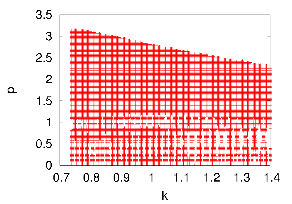
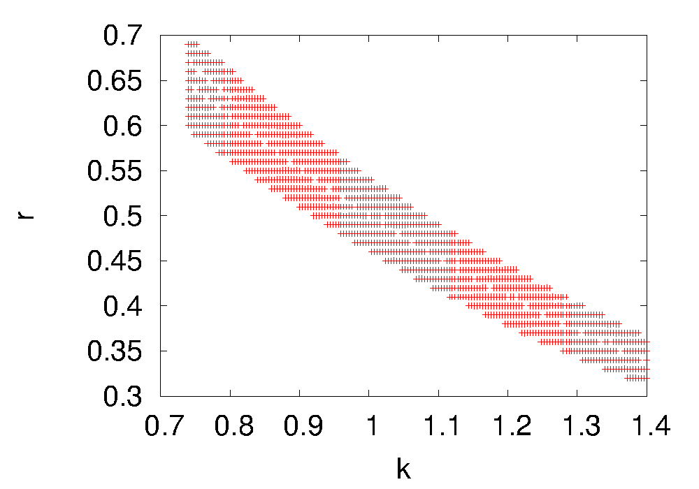
Figure 1: Allowed parameter space for ansatz conserving four zero cases given in Category A

IV Breaking of Scaling ansatz and generation of nonzero $\theta_{13}$

We want to break the scaling ansatz in such a way that
•   $\theta_{13}$ becomes nonzero.
•  Four zero structure is also retained.

The second assumption rules out all Category B textures as we have mentioned earlier. Breaking of scaling ansatz can only be incorporated in the remaining six four zero textures in Category A and after breaking the scaling ansatz by a dimensionless real parameter $\epsilon$ their structure come out as follows

$$m_{D}^{IA}=\left(\begin{array}[]{ccc}0&a&0\\ 0&kb(1+\epsilon)&kc\\ 0&b&c\end{array}\right),m_{D}^{IIA}=\left(\begin{array}[]{ccc}0&0&a\\ 0&kb&kc(1+\epsilon)\\ 0&b&c\end{array}\right),m_{D}^{IIIA}=\left(\begin{array}[]{ccc}a&0&0\\ kb(1+\epsilon)&0&kc\\ b&0&c\end{array}\right),$$ (61)

$$m_{D}^{IVA}=\left(\begin{array}[]{ccc}0&0&a\\ kb&0&kc(1+\epsilon)\\ b&0&c\end{array}\right),m_{D}^{VA}=\left(\begin{array}[]{ccc}a&0&0\\ kb(1+\epsilon)&kc&0\\ b&c&0\end{array}\right),m_{D}^{VIA}=\left(\begin{array}[]{ccc}0&a&0\\ kb&kc(1+\epsilon)&0\\ b&c&0\end{array}\right).$$

(62)

Theses structures of $m_{D}$ are free from RG effects which we have discussed in Appendix-A. Moreover, the breaking considered here are the most general which can be understood as follows: Consider the matrix $m_{D}^{IA}$ in which the breaking scheme is incorporated as

$${(m_{D})}_{\mu 2}=k(1+\epsilon){(m_{D})}_{\tau 2}$$ (63)

while

$${(m_{D})}_{\mu 3}=k{(m_{D})}_{\tau 3}.$$ (64)

Now, redefining the parameters $k(1+\epsilon)\rightarrow k$ and $-\epsilon\rightarrow\epsilon$ it is equivalent to break the ansatz in ${(m_{D})}_{\mu 3}$ and ${(m_{D})}_{\tau 3}$ elements. Proof of this equivalence is similar for other remaining five $m_{D}$ matrices. The effective neutrino mass matrix $m_{\nu}$ is same for all of them and is given by

$$m_{\nu}=m_{0}\left(\begin{array}[]{ccc}1&kp+kp\epsilon&p\\ kp+kp\epsilon&k^{2}re^{i\alpha}+2k^{2}p^{2}\epsilon&kre^{i\alpha}+kp^{2}\epsilon\\ p&kre^{i\alpha}+kp^{2}\epsilon&re^{i\alpha}\end{array}\right)$$ (65)

with the same definitions of the parameters ($k$, $p$, $r$, $\alpha$) that we have already used in eqns.(27) and (32).
We now rewrite this $m_{\nu}$ by breaking it in two parts, one $\epsilon$ dependent and the other independent of $\epsilon$, i.e

$$m_{\nu}=m_{0}\left(\begin{array}[]{ccc}1&kp&p\\ kp&k^{2}re^{i\alpha}&kre^{i\alpha}\\ p&kre^{i\alpha}&re^{i\alpha}\end{array}\right)+\epsilon m_{0}\left(\begin{array}[]{ccc}0&kp&0\\ kp&2k^{2}p^{2}&kp^{2}\\ 0&kp^{2}&0\end{array}\right)=m_{\nu}^{0}+\epsilon m_{\nu}^{\prime}$$ (66)

where we have denoted the first matrix in the right hand side of the above equation by $m_{\nu}^{0}$ and the second one by $m_{\nu}^{\prime}$. Computing $h_{t}$ using the above $m_{\nu}$, we get

$$h_{t}=m_{\nu}m_{\nu}^{\dagger}=m_{\nu}^{0}{m_{\nu}^{0}}^{\dagger}+\epsilon(m_{\nu}^{0}{m_{\nu}^{\prime}}^{\dagger}+m_{\nu}^{\prime}{m_{\nu}^{0}}^{\dagger})=h^{0}+\epsilon h^{p}$$ (67)

neglecting O($\epsilon^{2})$ terms. It is to be noted that $h^{0}$ is same as $h$, that we have obtained in eq.(33). After rotating out the phase $\phi$ appearing in $h^{0}$ we are left with

$$h_{t}^{\prime}=m_{0}^{2}\begin{pmatrix}A&k\arrowvert B\arrowvert&\arrowvert B\arrowvert\cr k\arrowvert B\arrowvert&k^{2}C&kC\cr\arrowvert B\arrowvert&kC&C\cr\end{pmatrix}+\epsilon h^{\prime\prime}$$ (68)

where $h^{\prime\prime}=diag(e^{i\phi},1,1)$ $h^{p}$ $diag(e^{-i\phi},1,1)$ and $h_{t}^{\prime}=diag(e^{i\phi},1,1)$ $h_{t}$ $diag(e^{-i\phi},1,1)$. To diagonalise $h_{t}^{\prime}$ we first rotate this matrix with unperturbed diagonalising matrix $U$ in eq. (38) with angles in eq. (39). The first part of $h_{t}^{\prime}$ becomes diagonal, however, the $h^{\prime\prime}$ part is not. Performing the operation $U^{\dagger}h_{t}^{\prime}U$ we get

$${h_{t}}^{\prime\prime}=U^{\dagger}h_{t}^{\prime}U=\begin{pmatrix}m_{1}^{2}&0&0\cr 0&m_{2}^{2}&0\cr 0&0&0\cr\end{pmatrix}+\epsilon\begin{pmatrix}x&y&z\cr y^{\ast}&w&q\cr z^{\ast}&q^{\ast}&0\cr\end{pmatrix}$$ (69)

where different elements of the the 2nd matrix are obtained from the explicit multiplication $U^{\dagger}h^{\prime\prime}U$. To diagonalise the second matrix of $h_{t}^{\prime\prime}$ we further require the matrix

$$U_{\epsilon}=\begin{pmatrix}1&\epsilon a&\epsilon b\cr-\epsilon a^{\ast}&1&\epsilon c\cr-\epsilon b^{\ast}&-\epsilon c^{\ast}&1\cr\end{pmatrix}.$$ (70)

Explicit expressions of parameters $x$, $y$, $z$, $q$ and $w$ are given in Appendix B. We demand that upto O($\epsilon$)the above matrix diagonalises $h_{t}^{\prime\prime}$ of eq.(69), i.e after the operation ${U_{\epsilon}}^{\dagger}{h_{t}}^{\prime\prime}U_{\epsilon}$ the off-diagonal elements of the resulting matrix are zero and solving those equations we find out the unknown variables $a$, $b$, $c$. They come out as

$$a=\frac{y}{(m_{2}^{2}-m_{1}^{2})}$$

$$b=-\frac{z}{m_{1}^{2}}$$

$$c=-\frac{q}{m_{2}^{2}}.$$ (71)

As a result of this rotation by the matrix $U_{\epsilon}$ we get

$$U_{\epsilon}^{\dagger}h_{t}^{\prime\prime}U_{\epsilon}=\begin{pmatrix}m_{1}^{2}+\epsilon x&0&0\cr 0&m_{2}^{2}+\epsilon w&0\cr 0&0&0\cr\end{pmatrix}.$$ (72)

In a concise way, we actually have done the following

$$U_{\epsilon}^{\dagger}U^{\dagger}h_{t}^{\prime}UU_{\epsilon}=\begin{pmatrix}m_{1}^{2}+\epsilon x&0&0\cr 0&m_{2}^{2}+\epsilon w&0\cr 0&0&0\cr\end{pmatrix}=\begin{pmatrix}{m_{1}^{\prime}}^{2}&0&0\cr 0&{m_{2}^{\prime}}^{2}&0\cr 0&0&{m_{3}^{\prime}}^{2}\cr\end{pmatrix}$$ (73)

where $m_{1}^{\prime}$, $m_{2}^{\prime}$, $m_{3}^{\prime}$ are the new mass eigenvalues. $m_{3}^{\prime}$ is still zero even after breaking of scaling ansatz because one column remain zero for all allowed $m_{D}$. Hence, the total diagonalisation matrix in our scheme is $V=UU_{\epsilon}$. Explicitly $V$ is given by

$$\small{V=\begin{pmatrix}c_{12}+s_{12}(\frac{\epsilon y^{\ast}}{m_{1}^{2}-m_{2}^{2}})&s_{12}+c_{12}(\frac{\epsilon y}{m_{2}^{2}-m_{1}^{2}})&-c_{12}(\frac{\epsilon z}{m_{1}^{2}})-s_{12}(\frac{\epsilon q}{m_{2}^{2}})\cr&&\cr-c_{23}s_{12}+c_{12}c_{23}(\frac{\epsilon y^{\ast}}{m_{1}^{2}-m_{2}^{2}})&-c_{23}s_{12}(\frac{\epsilon y}{m_{2}^{2}-m_{1}^{2}})+c_{12}c_{23}&c_{23}s_{12}(\frac{\epsilon z}{m_{1}^{2}})-c_{12}c_{23}(\frac{\epsilon q}{m_{2}^{2}})\cr+s_{23}(\frac{\epsilon z^{\ast}}{m_{1}^{2}})&+s_{23}(\frac{\epsilon q^{\ast}}{m_{2}^{2}})&+s_{23}\cr&&\cr s_{23}s_{12}-s_{23}c_{12}(\frac{\epsilon y^{\ast}}{m_{1}^{2}-m_{2}^{2}})&s_{23}s_{12}(\frac{\epsilon y}{m_{2}^{2}-m_{1}^{2}})-s_{23}c_{12}&-s_{23}s_{12}(\frac{\epsilon z}{m_{1}^{2}})+s_{23}c_{12}(\frac{\epsilon q}{m_{2}^{2}})\cr+c_{23}(\frac{\epsilon z^{\ast}}{m_{1}^{2}})&+c_{23}(\frac{\epsilon q^{\ast}}{m_{2}^{2}})&+c_{23}\cr.\end{pmatrix}}$$

To find out the three mixing angles we have to compare $V$ with PMNS matrix. The $U_{\rm PMNS}$ is given by

$$U_{\rm PMNS}=\begin{pmatrix}c_{12}^{\prime}c_{13}^{\prime}&s_{12}^{\prime}c_{13}^{\prime}&s_{13}^{\prime}e^{-i\delta}\cr-s_{12}^{\prime}c_{23}^{\prime}-c_{12}^{\prime}s_{23}^{\prime}s_{13}^{\prime}e^{i\delta}&c_{12}^{\prime}c_{23}^{\prime}-s_{12}^{\prime}s_{23}^{\prime}s_{13}^{\prime}e^{i\delta}&s_{23}^{\prime}c_{13}^{\prime}\cr s_{12}^{\prime}s_{23}^{\prime}-c_{12}^{\prime}c_{23}^{\prime}s_{13}^{\prime}e^{i\delta}&-c_{12}^{\prime}s_{23}^{\prime}-s_{12}^{\prime}c_{23}^{\prime}s_{13}^{\prime}e^{i\delta}&c_{23}^{\prime}c_{13}^{\prime}\cr\end{pmatrix}\begin{pmatrix}e^{i\alpha_{M}}&0&0\cr 0&e^{i\beta_{M}}&0\cr 0&0&1,\end{pmatrix}$$ (75)

(with $c_{ij}^{\prime}=cos\,\theta_{ij}^{\prime}$, $s_{ij}^{\prime}=sin\,\theta_{ij}^{\prime}$, $\delta$ is the Dirac phase and $\alpha_{M}$, $\beta_{M}$ are the Majorana phases.)
After neglecting the higher order terms in $\epsilon$ the modified mixing angles are given by

$$\tan\theta_{23}^{\prime}=\frac{\left|V_{23}\right|}{\left|V_{33}\right|}\approx t_{23}+\epsilon(1+t_{23}^{2})(\frac{s_{12}}{m_{1}^{2}}Re(z)-\frac{c_{12}}{m_{2}^{2}}Re(q))$$

$$\tan\theta_{12}^{\prime}=\frac{\left|V_{12}\right|}{\left|V_{11}\right|}\approx t_{12}+\epsilon(1+t_{12}^{2})\frac{Re(y)}{(m_{2}^{2}-m_{1}^{2})}$$

$$\sin\theta_{13}^{\prime}=\left|V_{13}\right|\approx\epsilon\sqrt{(\frac{c_{12}}{m_{1}^{2}}Re(z)+\frac{s_{12}}{m_{2}^{2}}Re(q))^{2}+(\frac{c_{12}}{m_{1}^{2}}Im(z)+\frac{s_{12}}{m_{2}^{2}}Im(q))^{2}}$$

and the CP violating phase $\delta$ is given by

$$\tan\delta=\frac{\frac{c_{12}}{m_{1}^{2}}Im(z)+\frac{s_{12}}{m_{2}^{2}}Im(q)}{\frac{c_{12}}{m_{1}^{2}}Re(z)+\frac{s_{12}}{m_{2}^{2}}Re(q)}$$ (77)

where $c_{ij}=\cos\theta_{ij}$, $s_{ij}=\sin\theta_{ij}$, $t_{ij}=\tan\theta_{ij}$ are the mixing angles and $m_{1}$, $m_{2}$ are the masses for the ansatz conserving case of eqn. (39) and eqn. (36) respectively. From eqn. (72) we have the mass squared differences:

$$(\Delta m_{21}^{2})^{\prime}=\Delta m_{21}^{2}+\epsilon(w-x)$$

$$(\Delta m_{32}^{2})^{\prime}=\Delta m_{32}^{2}-\epsilon w$$ (78)

where $\Delta m_{21}^{2}$ and $\Delta m_{32}^{2}$ are mass squared differences for unperturbed scaling ansatz as in eq. (40). The measure of CP violation is understood through $J_{CP}$ which is defined as

$$J_{\rm CP}=\frac{(h_{t})_{12}(h_{t})_{23}(h_{t})_{31}}{(\Delta m_{21}^{2})^{\prime}(\Delta m_{32}^{2})^{\prime}(\Delta m_{31}^{2})^{\prime}}$$ (79)

which is known function of $k$, $p$, $r$, $\alpha$ and $\epsilon$.

V Discussion of numerical results

We explore the parameter space of the above case using the same $3\sigma$ values of neutrino experimental data given in eqn.(41). The Lagrangian parameters $p$ and $r$ are ranging from zero to some positive values since we have separated out the phase part from them. The scale factor $k$ should not have zero value because in this case the second row of $(m_{D})$ is zero which in turn decouple the second generation. The constrained parameter space we obtain as

$$0<p<4$$

$$0.65<k<1.4$$

$$0<r<0.7$$

$$-180^{\circ}<\alpha<180^{\circ}.$$ (80)

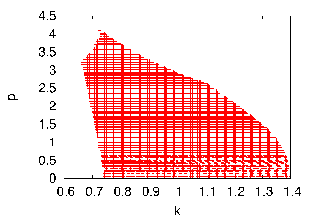
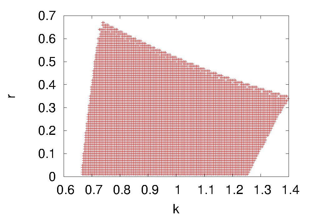
Figure 2: Allowed parameter space for $\epsilon=0.1$

The values outside this range is not admissible within the above mentioned experimental ranges. It is to be noted that allowed parameter space in $k$-$r$ plane for the ansatz breaking case is much larger than that in the ansatz conserving case. First of all, we found that throughout the allowed parameter space $\Sigma m_{i}$ and ${m_{\nu}}_{\beta\beta}$ are always far below the experimental bounds which could be hardly tested in the near future experiments. Next, it is amply clear from the expression of $\theta_{13}$ that it is directly proportional to the value of the ansatz breaking parameter $\epsilon$. The parameter $\epsilon$ is varied upto a reasonable choice $\epsilon=0.1$ for which a large $\theta_{13}$ is generated, however, for a smaller value of $\epsilon$ such as $\epsilon\sim 0.07$, $\theta_{13}\sim 10^{\circ}$ is also admitted because present experimental bound on $\theta_{13}$ is $3.75^{\circ}\leq\theta_{13}\leq 13.60^{\circ}$ for $3\sigma$ bound from RENO last and $4.90^{\circ}\leq\theta_{13}\leq 11.51^{\circ}$ for $3\sigma$ bound from Daya-Bay DayaBay . We have shown all plots for a representative value of $\epsilon=0.1$ . The allowed Lagrangian parameter space is plotted in Fig.2.

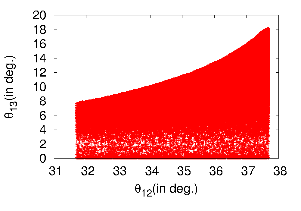
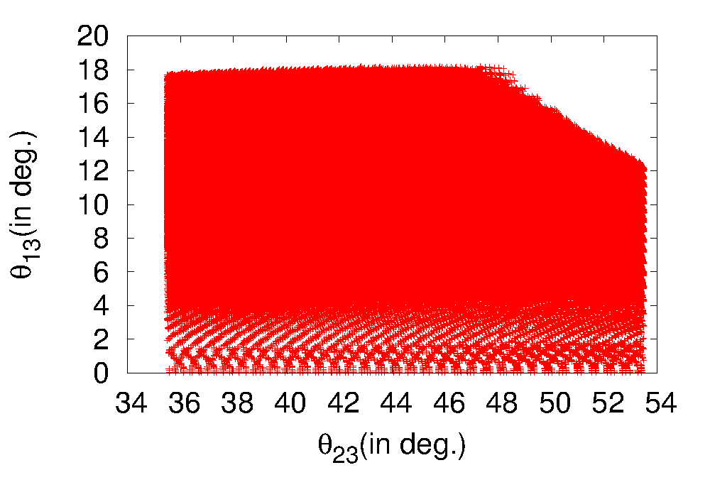
Figure 3: Allowed values of the mixing angles for $\epsilon=0.1$

From Fig.3 it is clear that $\theta_{13}$ is almost insensitive to $\theta_{23}$, however, significantly related to the values of $\theta_{12}$ which is depicted in Fig.3. The CP violation parameter $J_{cp}$ arises due to nonzero $\theta_{13}$ is plotted with $\theta_{13}$ in Fig.4. Sign of $\delta$ is not constrained from oscillation experiments it needs further calculation of baryon asymmetry. Plot (Fig.4) of $\theta_{13}$ vs $\delta$ shows that $\delta$ is maximum for smaller values of $\theta_{13}$ and for larger values of $\theta_{13}$, $\delta$ is relatively small. If we restrict $\theta_{13}$ in $3\sigma$ experimental range we have the bound on $\delta$, $0\leq\delta\leq 35^{\circ}$ and $J_{CP}$, $0\leq J_{CP}\leq 0.02$.

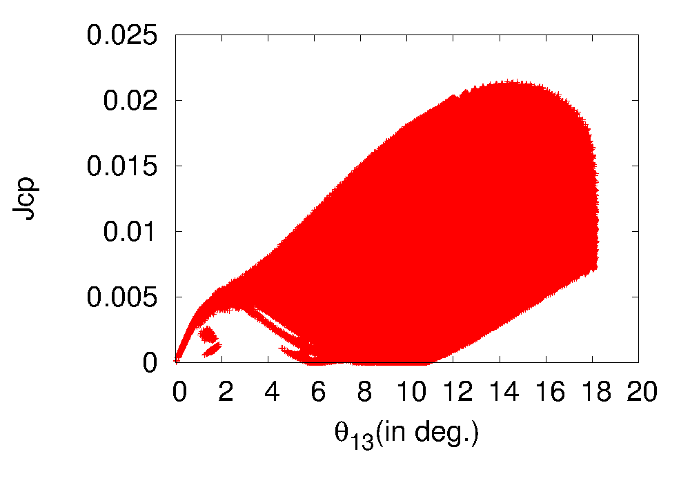
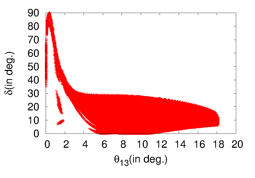
Figure 4: Allowed $\arrowvert\ J_{CP}\arrowvert$ vs $\theta_{13}$ (left), $\arrowvert\delta\arrowvert$ vs $\theta_{13}$(right) for $\epsilon=0.1$

VI Leptogenesis with broken scaling ansatz

VI.1 General discussion on Leptogenesis and Baryogenesis

Let us briefly discuss about right handed Majorana neutrino decay generated leptogenesis. There is a Dirac type Yukawa interaction of right handed neutrino (${N}_{i}$) with SM lepton doublet and Higgs doublet. At the energy scale where $SU(2)_{L}\times U(1)_{Y}$ symmetry is preserved, physical right handed neutrino ${N}_{i}$ with definite mass can decay both to charged lepton with charged scalar and light neutrino with neutral scalar. Due to the Majorana character of ${N}_{i}$, conjugate process is also possible. If out of equilibrium decay of ${N}_{i}$ in conjugate process occur at different rate from actual process, net lepton number will be generated. The CP asymmetry of decay is characterized by a parameter $\varepsilon_{i}$ which is defined as

$$\varepsilon_{i} = \frac{\Gamma_{{N}_{i}\rightarrow l^{-}\phi^{+},\nu_{l}\phi^{0}}-\Gamma_{{N}_{i}\rightarrow l^{+}\phi^{-},\nu_{l}^{c}\phi^{0*}}}{\Gamma_{{N}_{i}\rightarrow l^{-}\phi^{+},\nu_{l}\phi^{0}}+\Gamma_{{N}_{i}\rightarrow l^{+}\phi^{-},\nu_{l}^{c}\phi^{0*}}}.$$ (81)

We are working in a basis where right handed neutrinos have definite mass as , $M_{R}={\rm diag}(M_{1},M_{2},M_{3})$. Now, the decay asymmetry $\varepsilon_{i}$ for $N_{i}$ decay occurs at one loop level. Interference of tree level, one loop vertex and self energy diagrams generate the following $\varepsilon_{i}$ for hierarchical right handed neutrino mass spectrum:

$$\varepsilon_{i}=\frac{1}{4\pi v^{2}H_{ii}}\sum_{j\neq i}Im(H_{ij}^{2})f(x_{ij})$$ (82)

where $x_{ij}=M_{j}^{2}/M_{i}^{2}$, $H=m_{D}^{\dagger}m_{D}$ and Covi:1996wh

$$f(x)=\sqrt{x}\left\{1-(1+x)\ln(1+\frac{1}{x})+\frac{1}{1-x}\right\}.$$ (83)

CP asymmetry parameters $\varepsilon_{i}$ are related to the leptonic asymmetry parameters through $Y_{L}$ as Nielsen:2001fy ; Pilaftsis:2003gt ; Antusch:2006cw

$$Y_{L}\equiv\frac{n_{L}-{\bar{n}}_{L}}{s}=\sum_{i}^{3}\frac{\varepsilon_{i}\kappa_{i}}{g_{*i}}$$ (84)

where $n_{L}$ is the lepton number density, ${\bar{n}}_{L}$ is the anti-lepton number density, $s$ is the entropy density, $\kappa_{i}$ is the dilution factor for the CP asymmetry $\varepsilon_{i}$ and $g_{*i}$ is the effective number of degrees of freedom Roos:1994fz at temperature $T=M_{i}$. The baryon asymmetry $Y_{B}$ produced through the sphaleron transmutation of $Y_{L}$, while the quantum number $B-L$ remains conserved, is given by Harvey:1990qw

$$Y_{B}=-\frac{8N_{F}+4N_{H}}{22N_{F}+13N_{H}}Y_{L}$$ (85)

where $N_{F}$ is the number of fermion families and $N_{H}$ is the number of Higgs doublets. The quantity $Y_{B}=-\frac{28}{79}Y_{L}$ in eq. (85) for SM. Now we introduce the relation between $Y_{B}$ and $\eta_{B}$, where $\eta_{B}$ is the baryon number density over photon number density $n_{\gamma}$. The relation is Kolb

$$\eta_{B}=\left.\frac{s}{n_{\gamma}}\right|_{0}Y_{B}=7.0394Y_{B},$$ (86)

where the zero indicates present time. Finally we have relation between $\eta_{B}$ and $\varepsilon_{i}$

$$\eta_{B}=-2.495\times\sum_{i}\frac{\varepsilon_{i}\kappa_{i}}{g_{*i}}.$$ (87)

This dilution factor $\kappa_{i}$ approximately given by Giudice:2003jh ; Buchmuller:2004nz ; Abada:2006ea

$$\frac{1}{\kappa_{i}}\simeq\frac{8.25}{K_{i}}+\left(\frac{K_{i}}{0.2}\right)^{1.16}\qquad{\rm with}\qquad K_{i}=\frac{\Gamma_{i}}{H_{i}},$$ (88)

where $\Gamma_{i}$ is the decay width of $N_{i}$ and $H_{i}$ is Hubble constant at $T=M_{i}$. Their expressions are

$$\Gamma_{i}=\frac{h_{ii}M_{i}}{4\pi v^{2}}\qquad{\rm and}\qquad H_{i}=1.66\sqrt{g_{*i}}\frac{M_{i}^{2}}{M_{P}},$$ (89)

where $v=246$GeV and $M_{P}=1.22\times 10^{19}$GeV. Thus we have

$$K_{i}=\frac{M_{P}H_{ii}}{1.66\times 4\pi\sqrt{g_{*i}}v^{2}M_{i}}.$$ (90)

VI.2 Calculation of lepton and baryon asymmetry with broken scaling ansatz

The matrix $H=m_{D}^{\dagger}m_{D}$ shown in eq. (82) is important to study leptogenesis. For six possible $m_{D}$ with broken scaling ansatz by parameter $\epsilon$ are given in eq. 62. They will generate following six possible $H$ in three pairs:

$$m_{0}M_{2}\left(\begin{array}[]{ccc}0&0&0\\ 0&1+p^{2}(1+k^{2})+2p^{2}k^{2}\epsilon&lpqe^{i(\beta-\theta)}(1+k^{2}+k^{2}\epsilon)\\ 0&lpqe^{-i(\beta-\theta)}(1+k^{2}+k^{2}\epsilon)&q^{2}l^{2}(1+k^{2})\end{array}\right)\quad{\rm with}\quad l=\sqrt{\frac{M_{3}}{M_{2}}}$$ (94)

$$m_{0}M_{3}\left(\begin{array}[]{ccc}0&0&0\\ 0&q^{2}l^{2}(1+k^{2})&lpqe^{-i(\beta-\theta)}(1+k^{2}+k^{2}\epsilon)\\ 0&lpqe^{i(\beta-\theta)}(1+k^{2}+k^{2}\epsilon)&1+p^{2}(1+k^{2})+2p^{2}k^{2}\epsilon\end{array}\right)\quad{\rm with}\quad l=\sqrt{\frac{M_{2}}{M_{3}}}$$ (98)

(99)

$$m_{0}M_{1}\left(\begin{array}[]{ccc}1+p^{2}(1+k^{2})+2p^{2}k^{2}\epsilon&0&lpqe^{i(\beta-\theta)}(1+k^{2}+k^{2}\epsilon)\\ 0&0&0\\ lpqe^{-i(\beta-\theta)}(1+k^{2}+k^{2}\epsilon)&0&q^{2}l^{2}(1+k^{2})\end{array}\right)\quad{\rm with}\quad l=\sqrt{\frac{M_{3}}{M_{1}}}$$ (103)

$$m_{0}M_{3}\left(\begin{array}[]{ccc}q^{2}l^{2}(1+k^{2})&0&lpqe^{-i(\beta-\theta)}(1+k^{2}+k^{2}\epsilon)\\ 0&0&0\\ lpqe^{i(\beta-\theta)}(1+k^{2}+k^{2}\epsilon)&0&1+p^{2}(1+k^{2})+2p^{2}k^{2}\epsilon\end{array}\right)\quad{\rm with}\quad l=\sqrt{\frac{M_{1}}{M_{3}}}$$ (107)

$$m_{0}M_{1}\left(\begin{array}[]{ccc}1+p^{2}(1+k^{2})+2p^{2}k^{2}\epsilon&lpqe^{i(\beta-\theta)}(1+k^{2}+k^{2}\epsilon)&0\\ lpqe^{-i(\beta-\theta)}(1+k^{2}+k^{2}\epsilon)&q^{2}l^{2}(1+k^{2})&0\\ 0&0&0\end{array}\right)\quad{\rm with}\quad l=\sqrt{\frac{M_{2}}{M_{1}}}$$ (112)

$$m_{0}M_{2}\left(\begin{array}[]{ccc}q^{2}l^{2}(1+k^{2})&lpqe^{-i(\beta-\theta)}(1+k^{2}+k^{2}\epsilon)&0\\ lpqe^{i(\beta-\theta)}(1+k^{2}+k^{2}\epsilon)&1+p^{2}(1+k^{2})+2p^{2}k^{2}\epsilon&0\\ 0&0&0\end{array}\right)\quad{\rm with}\quad l=\sqrt{\frac{M_{1}}{M_{2}}}.$$ (116)

Parameters in above six possible $H$ are already defined in eq.(27) and only $l$ is defined here along with every $H$. Interesting features of the three pairs of $H$ are that for every pair one generation of right handed neutrino decouples and also its decay width vanishes and hence could not take part in generation of lepton asymmetry. For the first pair $N_{1}$ decouples, for the 2nd pair $N_{2}$ decouples and for the 3rd pair $N_{3}$ decouples. Apart from this one more interesting point is that first matrix of every pair have similar expression in their non-zero diagonal and off-diagonal elements whereas the 2nd matrix of every pair have similar expressions. So, we don’t need to study all the three pairs. We will only study the first pair.

First generation of right handed neutrino $N_{1}$ decay width is zero. Lepton asymmetry is generated through decay of $N_{2}$ and $N_{3}$ only contribute. Decay asymmetries $\varepsilon_{2}$ and $\varepsilon_{3}$ for the first form of the first pair in eq. (99),

$$\varepsilon_{2}=\frac{1}{4\pi v^{2}}\frac{{\rm Im}(H_{23}^{2})}{H_{22}}f(M_{3}^{2}/M_{2}^{2})=\frac{M_{2}m_{0}}{4\pi v^{2}}Ff(l^{4})$$

$$\varepsilon_{3}=\frac{1}{4\pi v^{2}}\frac{{\rm Im}(H_{32}^{2})}{H_{33}}f(M_{2}^{2}/M_{3}^{2})=-\frac{M_{2}m_{0}}{4\pi v^{2}}F^{\prime}f(1/l^{4})$$ (118)

where $l=\sqrt{\frac{M_{3}}{M_{2}}}$ and

$$F=\frac{rl^{2}p^{2}(1+k^{2})\sin\alpha}{1+p^{2}(1+k^{2})}\left[1+k^{2}+\frac{2k^{2}\epsilon}{1+p^{2}(1+k^{2})}\right]$$

$$F^{\prime}=\frac{rp^{2}(1+k^{2})\sin\alpha}{(1+k^{2})\sqrt{p^{4}+r^{2}-2rp^{2}\cos\alpha}}\left[1+k^{2}+2k^{2}\epsilon\right].$$ (119)

The definition of different parameters for different $m_{D}$ are given in eq. 27 and also we have used $q^{2}e^{2i(\beta-\theta)}=re^{i\alpha}-p^{2}$. The washout factors for 2nd and 3rd generation are

$$K_{2}=\frac{M_{P}H_{22}}{1.66\times 4\pi\sqrt{g_{*2}}v^{2}M_{2}}=913.7\left(\frac{m_{0}}{\rm eV}\right)\left[1+p^{2}(1+k^{2}+2k^{2}\epsilon)\right]$$

$$K_{3}=\frac{M_{P}H_{33}}{1.66\times 4\pi\sqrt{g_{*3}}v^{2}M_{3}}=913.7\left(\frac{m_{0}}{\rm eV}\right)(1+k^{2})\sqrt{p^{4}+r^{2}-2rp^{2}\cos\alpha}.$$

(120)

where we have used $v=246$GeV, $M_{P}=1.22\times 10^{19}$GeV and $g_{*i}=110.25$ for SM with two right handed neutrinos. With this washout factors we can determine the dilution factors $\kappa_{2}$ and $\kappa_{3}$ using the formula given in eq. 88. Well equipped with the above formulae for $\varepsilon_{2}$, $\varepsilon_{3}$, $\kappa_{2}$ and $\kappa_{3}$ we can easily generate the expression for baryon asymmetry

$$\eta_{B} = -2.495\times\sum_{i}\frac{\varepsilon_{i}\kappa_{i}}{g_{*i}}$$ (121)

$$= -2.27\times 10^{-2}\left[\varepsilon_{2}\kappa_{2}+\varepsilon_{3}\kappa_{3}\right].$$

An additional beauty is that the expressions for $\eta_{B}$ for two matrices in a pair are same. For the 2nd matrix of the first pair in eq. (99), expressions for $\varepsilon_{2}$ and $K_{2}$ are same as the expressions of $\varepsilon_{3}$ and $K_{3}$ for the first matrix of the pair and expressions for $\varepsilon_{3}$ and $K_{3}$ are same as the expressions of $\varepsilon_{2}$ and $K_{2}$ of first matrix of the pair. So, effectively $\eta_{B}$ expression remains same. Consequence is same as for the first matrix of the pair.

The expression of $\eta_{B}$ depends on $m_{0}$, $k$, $p$, $r$, $\alpha$, $\epsilon$ and additional two parameters $M_{2}$ and $l=\sqrt{\frac{M_{3}}{M_{2}}}$. On the top of constrained parameter space from neutrino data, we have also explored the parameter space with the additional constraint arises due to baryon asymmetry $5.5\times 10^{-10}<\eta_{b}<7\times 10^{-10}$ bary1 ; bary2 ; bary3 for $0.1\leq l\leq 0.9$ and $1.1\leq l\leq 10$ (avoiding point of degeneracy $l=1$) and $10^{12}~{}{\rm GeV}\leq M_{2}\leq 10^{15}~{}{\rm GeV}$. We have seen that change in the parameter space is negligible. Only sign of $\alpha$ is constrained for different $l$. For $1.1\leq l\leq 1.54$ and $0.1\leq l\leq 0.9$ sign of $\alpha$ is negative and for $1.54\leq l\leq 10$ sign of $\alpha$ is positive. Again $\alpha=0,\pm 180$ are not allowed. But value of $\alpha$ near $0$ and $180$ are still allowed and the $M_{2}$ value is large there, $M_{2}\simeq O(10^{15})$ GeV.

VII Summary

To sum up, we have explored a predictive and testable scenario of neutrino mass matrix accommodating scaling ansatz with four zero Yukawa textures advocating type I seesaw mechanism with diagonal charged leptons and right chiral neutrino mass matrices. We break scaling ansatz in the Yukawa matrices to generate nonzero $\theta_{13}$ through a dimensionless parameter $\epsilon$. The parameter space of the textures studied allow the $3\sigma$ value of $\theta_{13}$ along with other neutrino experimental data. Using the $\theta_{13}$ constraint we have restricted Dirac CP phase $\delta$ and $J_{CP}$. We have also studied baryogenesis via leptogenesis arises in those textures, however, there is no drastic change in the parameter space due to the constraint from baryogenesis. But, the sign of the only phase present in this model is fixed.

Acknowledgement
Authors would like to thanks Probir Roy, Debabrata Adak and Anirban Biswas for many helpful discussions.

Appendix A RG Effect

It is to be noted that even after breaking of scaling anasatz, the textures given in eqn.(62) are invariant under RG evolution. This is guaranteed in the following way : Following the methodology presented in Ref.rg1 - rg2 due to $\tau$ lepton mass correction on $m_{D}$ of eqn. (5) with scaling ansatz we get

$$\begin{pmatrix}1&0&0\cr 0&1&0\cr 0&0&1-\Delta_{\tau}\end{pmatrix}\begin{pmatrix}a_{1}&a_{2}&a_{3}\cr kb_{1}&kb_{2}&kb_{3}\cr b_{1}&b_{2}&b_{3}\end{pmatrix}=\begin{pmatrix}a_{1}&a_{2}&a_{3}\cr kb_{1}&kb_{2}&kb_{3}\cr b_{1}(1-\Delta_{\tau})&b_{2}(1-\Delta_{\tau})&b_{3}(1-\Delta_{\tau})\par\end{pmatrix}.$$ (122)

Redifining $b_{i}$‘s as $b_{1}(1-\Delta_{\tau})\rightarrow b_{1}$, $b_{2}(1-\Delta_{\tau})\rightarrow b_{2}$, $b_{3}(1-\Delta_{\tau})\rightarrow b_{3}$ we get

$$m_{D}=\begin{pmatrix}a_{1}&a_{2}&a_{3}\cr kb_{1}(1+\Delta_{\tau})&kb_{2}(1+\Delta_{\tau})&kb_{3}(1+\Delta_{\tau})\cr b_{1}&b_{2}&b_{3}\par\end{pmatrix}$$ (123)

where we consider ${(1-\Delta_{\tau})}^{-1}\approx 1+\Delta_{\tau}$ since $\Delta_{\tau}$ is far less than unity. If we consider $k(1+\Delta_{\tau})\rightarrow k$ then, we get the structure of $m_{D}$ given in eqn.(5). So, $m_{D}$ with scaling ansatz remains form invariant including RG effect. Now, if we consider scaling ansatz breaking through $\epsilon$ parameter, the structure of $m_{D}$ comes out as

$$m_{D}=\begin{pmatrix}a_{1}&a_{2}&a_{3}\cr kb_{1}&kb_{2}(1+\epsilon)&kb_{3}\cr b_{1}&b_{2}&b_{3}\end{pmatrix}.$$ (124)

Again, RG effect through parameter $\Delta_{\tau}$ on $m_{D}$ with broken scaling ansatz is given by

$$\begin{pmatrix}1&0&0\cr 0&1&0\cr 0&0&(1-\Delta)\end{pmatrix}\begin{pmatrix}a_{1}&a_{2}&a_{3}\cr kb_{1}&kb_{2}(1+\epsilon)&kb_{3}\cr b_{1}&b_{2}&b_{3}\end{pmatrix}=\begin{pmatrix}a_{1}&a_{2}&a_{3}\cr kb_{1}&kb_{2}(1+\epsilon)&kb_{3}\cr b_{1}(1-\Delta_{\tau})&b_{2}(1-\Delta_{\tau})&b_{3}(1-\Delta_{\tau})\par\end{pmatrix}.$$ (125)

Performing the same exercise of redefinition of $b_{i}$’s and $k$, the same $m_{D}$ is obtained as in eq.(124). So, the structure of $m_{D}$ matrices with broken scaling ansatz in eq.(62) are free from RG effect.

Appendix B Expressions used in Sec-4

In our calculation we have written $m_{\nu}$ by breaking it into two parts, i.e

$$m_{\nu}=m_{\nu}^{0}+\epsilon m_{\nu}^{\prime}.$$ (126)

If we assume a generic form of $m_{\nu}^{\prime}$ as

$$m_{\nu}^{\prime}=m_{0}\left(\begin{array}[]{ccc}A_{1}&B_{1}&C_{1}\\ B_{1}&B_{2}&C_{2}\\ C_{1}&C_{2}&C_{3}\end{array}\right)$$ (127)

(In our case $A_{1}=0$, $B_{1}=kp$, $C_{1}=0$, $B_{2}=2k^{2}p^{2}$, $C_{2}=kp^{2}$, $C_{3}=0$.)
The different elements of the matrix $h^{p}$ in terms of the parameters ($k$, $p$, $r$, $\alpha$) are given by

$$h^{p}_{11}=m_{0}^{2}(2Re(A_{1})+2kpRe(B_{1})+2pRe(C1))$$ (128)

$$h^{p}_{12}=m_{0}^{2}(B_{1}^{\ast}+kpB_{2}^{\ast}+pC_{2}^{\ast}+A_{1}kp+B_{1}k^{2}re^{-i\alpha}+C_{1}kre^{-i\alpha})$$ (129)

$$h^{p}_{13}=m_{0}^{2}(C_{1}^{\ast}+kpC_{2}^{\ast}+pC_{3}^{\ast}+A_{1}p+B_{1}kre^{-i\alpha}+C_{1}re^{-i\alpha})$$ (130)

$$h^{p}_{22}=m_{0}^{2}(2kpRe(B_{1})+2k^{2}r(Re(B_{2})\cos\alpha+Im(B_{2})\sin\alpha)+2kr(Re(C_{2})\cos\alpha$$

$$+Im(C_{2})\sin\alpha))$$ (131)

$$h^{p}_{23}=m_{0}^{2}(kpC_{1}^{\ast}+k^{2}re^{i\alpha}C_{2}^{\ast}+kre^{i\alpha}C_{3}^{\ast}+B_{1}p+B_{2}kre^{-i\alpha}+C_{2}re^{-i\alpha})$$ (132)

$$h^{p}_{33}=m_{0}^{2}(2pRe(C_{1})+2kr(Re(C_{2})\cos\alpha+Im(C_{2})\sin\alpha)+2r(Re(C_{3})\cos\alpha$$

$$+Im(C_{3})\sin\alpha))$$ (133)

Parameters like $x$, $y$, $z$, etc can be expressed in terms of different elements of $h^{p}$ matrix as

$$x=c_{12}(h^{p}_{11}c_{12}-h^{p}_{12}e^{i\phi}c_{23}s_{12}+h^{p}_{13}e^{i\phi}s_{23}s_{12})-c_{23}s_{12}(h^{p^{\ast}}_{12}e^{-i\phi}c_{12}-c_{23}s_{12}h^{p}_{22}+h^{p}_{23}s_{23}s_{12})$$

$$+s_{23}s_{12}(h^{p^{\ast}}_{13}e^{-i\phi}c_{12}-h^{p^{\ast}}_{23}e^{-i\phi}c_{23}s_{12}+h^{p}_{33}s_{23}s_{12})$$ (134)

$$y=c_{12}(h^{p}_{11}s_{12}+h^{p}_{12}e^{i\phi}c_{12}c_{23}-h^{p}_{13}e^{i\phi}s_{23}c_{12})-c_{23}s_{12}(h^{p^{\ast}}_{12}e^{-i\phi}s_{12}+h^{p}_{22}c_{12}c_{23}-h^{p}_{23}s_{23}c_{12})$$

$$+s_{23}s_{12}(h^{p^{\ast}}_{13}e^{-i\phi}s_{12}+h^{p^{\ast}}_{23}e^{-i\phi}c_{12}c_{23}-h^{p}_{33}s_{23}c_{12})$$ (135)

$$z=c_{12}(h^{p}_{12}e^{i\phi}s_{23}+h^{p}_{13}e^{i\phi}c_{23})-c_{23}s_{12}(h^{p}_{22}s_{23}+h^{p}_{23}c_{23})+s_{23}s_{12}(h^{p^{\ast}}_{23}e^{-i\phi}s_{23}+h^{p}_{33}c_{23})$$ (136)

$$w=s_{12}(h^{p}_{11}s_{12}+h^{p}_{12}e^{i\phi}c_{12}c_{23}-h^{p}_{13}e^{i\phi}s_{23}c_{12})+c_{12}c_{23}(h^{p^{\ast}}_{12}e^{-i\phi}s_{12}+h^{p}_{22}c_{12}c_{23}-h^{p}_{23}s_{23}c_{12})$$

$$-s_{23}c_{12}(h^{p^{\ast}}_{13}e^{-i\phi}s_{12}+h^{p^{\ast}}_{23}e^{-i\phi}c_{12}c_{23}-h^{p}_{33}s_{23}c_{12})$$ (137)

$$q=s_{12}(h^{p}_{12}e^{i\phi}s_{23}+h^{p}_{13}e^{i\phi}c_{23})+c_{12}c_{23}(h^{p}_{22}s_{23}+h^{p}_{23}c_{23})-s_{23}c_{12}(h^{p^{\ast}}_{23}e^{-i\phi}s_{23}+h^{p}_{33}c_{23})$$ (138)

References

• (1) J. Gluza and R. Szafron, Phys. Rev. D 85 (2012) 047701 [arXiv:1111.7278 [hep-ph]].
• (2) X. -G. He and S. K. Majee, JHEP 1203, 023 (2012) [arXiv:1111.2293 [hep-ph]].
• (3) G. Mangano, G. Miele, S. Pastor, O. Pisanti and S. Sarikas, Phys. Lett. B 708 (2012) 1 [arXiv:1110.4335 [hep-ph]].
• (4) Q. -H. Cao, S. Khalil, E. Ma and H. Okada, Phys. Rev. D 84 (2011) 071302 [arXiv:1108.0570 [hep-ph]].
• (5) W. Chao and Y. -j. Zheng, arXiv:1107.0738 [hep-ph].
• (6) D. Meloni, JHEP 1110 (2011) 010 [arXiv:1107.0221 [hep-ph]].
• (7) N. Haba and R. Takahashi, Phys. Lett. B 702 (2011) 388 [arXiv:1106.5926 [hep-ph]].
• (8) A. B. Balantekin, J. Phys. Conf. Ser.  337 (2012) 012049 [arXiv:1106.5021 [hep-ph]].
• (9) S. Zhou, Phys. Lett. B 704 (2011) 291 [arXiv:1106.4808 [hep-ph]]. P. Novella and f. t. D. C. collaboration, arXiv:1105.6079 [hep-ex].
• (10) A. B. Balantekin, AIP Conf. Proc.  1269 (2010) 195 [arXiv:1006.2836 [nucl-th]].
• (11) M. C. Gonzalez-Garcia, M. Maltoni and J. Salvado, JHEP 1004,(2010) 056 [arXiv:1001.4524 [hep-ph]].
• (12) E. E. Jenkins and A. V. Manohar, Phys. Lett. B 668 (2008) 210 [arXiv:0807.4176 [hep-ph]].
• (13) A. B. Balantekin and D. Yilmaz, J. Phys. G G 35 (2008) 075007 [arXiv:0804.3345 [hep-ph]].
• (14) V. Barger, R. Gandhi, P. Ghoshal, S. Goswami, D. Marfatia, S. Prakash, S. K. Raut and S U. Sankar, arXiv:1203.6012 [hep-ph].
• (15) Y. H. Ahn and S. K. Kang, arXiv:1203.4185 [hep-ph].
• (16) B. Brahmachari and A. Raychaudhuri, arXiv:1204.5619 [hep-ph].
• (17) X. G. He and S. K. Majee, JHEP 1203 (2012) 023 [arXiv:1111.2293 [hep-ph]].
• (18) H. Ishimori and E. Ma, arXiv : 1205.0075 [hep-ph].
• (19) [MINOS Collaboration] L. Whitehead, Joint Experimental-Theoretical Seminar (24 June 2011, Fermilab, USA). Websites: theory.fnal.gov/jetp, http://www-numi.fnal.gov/pr plots/ .
• (20) [MINOS Collaboration] P. Adamson et al., [arXiv:1108.0015 [hep-ex]].
• (21) [T2K Collaboration] K. Abe et al, Phys. Rev. Lett.  107 (2011) 041801 [arXiv:1106.2822 [hep-ex]].
• (22) H. De. Kerrect, Low Nu 2011, Seoul, South Korea, http://workshop.kias.re.kr/lownu11/ .
• (23) [DAYA-BAY Collaboration] F. P. An et al., Phys. Rev. Lett.  108 (2012) 171803 [arXiv:1203.1669 [hep-ex]].
• (24) [RENO Collaboration] J. K. Ahn et al., arXiv:1204.0626 [hep-ex].
• (25) A. S. Joshipura and W. Rodejohann, Phys. Lett. B 678 (2009) 276 [arXiv:0905.2126 [hep-ph]].
• (26) R. N. Mohapatra and W. Rodejohann, Phys. Lett. B 644 (2007) 59 [hep-ph/0608111].
• (27) A. Blum, R. N. Mohapatra and W. Rodejohann, Phys. Rev. D 76, 053003 (2007) [arXiv:0706.3801 [hep-ph]].
• (28) M. Obara, arXiv:0712.2628 [hep-ph].
• (29) A. Damanik, M. Satriawan, Muslim and P. Anggraita, arXiv:0705.3290 [hep-ph].
• (30) S. Goswami and A. Watanabe, Phys. Rev. D 79, 033004 (2009) [arXiv:0807.3438 [hep-ph]].
• (31) W. Grimus and L. Lavoura, J. Phys. G G 31, 683 (2005) [hep-ph/0410279].
• (32) M. S. Berger and S. Santana, Phys. Rev. D 74, 113007 (2006) [hep-ph/0609176].
• (33) S. Goswami, S. Khan and W. Rodejohann, Phys. Lett. B 680 (2009) 255 [arXiv:0905.2739 [hep-ph]].
• (34) G. C. Branco, D. Emmanuel-Costa, M. N. Rebelo and P. Roy, Phys. Rev. D 77 (2008) 053011 [arXiv:0712.0774 [hep-ph]].
• (35) S. Choubey, W. Rodejohann and P. Roy, Nucl. Phys. B 808, 272 (2009) [Erratum-ibid.  818, 136 (2009)] [arXiv:0807.4289 [hep-ph]].
• (36) B. Adhikary, A. Ghosal and P. Roy, JHEP 0910 (2009) 040 [arXiv:0908.2686 [hep-ph]].
• (37) B. Adhikary, A. Ghosal and P. Roy, JCAP 1101 (2011) 025 [arXiv:1009.2635 [hep-ph]].
• (38) B. Adhikary, A. Ghosal and P. Roy, Mod. Phys. Lett. A 26 (2011) 2427 [arXiv:1103.0665 [hep-ph]].
• (39) H. Fritzsch, Z. -z. Xing and S. Zhou, JHEP 1109 (2011) 083 [arXiv:1108.4534 [hep-ph]].
• (40) M. Maltoni and T. Schwetz, PoS IDM 2008 (2008) 072 [arXiv:0812.3161 [hep-ph]].
• (41) A. Damanik, arXiv:1201.2747 [hep-ph].
• (42) S. A. Thomas, F. B. Abdalla and O. Lahav, Phys. Rev. Lett.  105 (2010) 031301 [arXiv:0911.5291 [astro-ph.CO]].
• (43) M. C. Gonzalez-Garcia, M. Maltoni and J. Salvado, JHEP 1008 (2010) 117 [arXiv:1006.3795 [hep-ph]].
• (44) S. Parke, Unreavelling the neutrino mysteries: Present and future, Summary talk at NUFACT10, http://www.info.tifr.res.in/nufact2010/procedings.php/.
• (45) J. J. Gomez-Cadenas, J. Martin-Albo, M. Sorel, P. Ferrario, F. Monrabal, J. Munoz-Vidal, P. Novella and A. Poves, JCAP 1106 (2011) 007 [arXiv:1010.5112 [hep-ex]].
• (46) L. Covi, E. Roulet and F. Vissani, Phys. Lett. B 384 (1996) 169 [hep-ph/9605319].
• (47) H. B. Nielsen and Y. Takanishi, Phys. Lett. B 507 (2001) 241 [hep-ph/0101307].
• (48) A. Pilaftsis and T. E. J. Underwood, Nucl. Phys. B 692 (2004) 303 [hep-ph/0309342].
• (49) S. Antusch, S. F. King and A. Riotto, JCAP 0611 (2006) 011 [hep-ph/0609038].
• (50) M. Roos,Introduction to cosmology, Chichester, UK: Wiley (2003) p 279.
• (51) J. A. Harvey and M. S. Turner, Phys. Rev.  D 42 (1990) 3344.
• (52) E. W. Kolb and M. S. Turner, The Early Universe (Addison-Wesley, Redwood City, CA, U.S.A,) (1990).
• (53) G. F. Giudice, A. Notari, M. Raidal, A. Riotto and A. Strumia, Nucl.  Phys. B, 685 (2004) 89 [hep-ph/0310123].
• (54) W. Buchmuller, P. Di Bari and M. Plumacher, Annals Phys. 315 (2005) 305 [hep-ph/0401240].
• (55) A. Abada, S. Davidson, A. Ibarra, F. -X. Josse-Michaux, M. Losada and A. Riotto, JHEP 0609 (2006) 010 [hep-ph/0605281].
• (56) [WMAP Collaboration], D. N. Spergel et al., Astrophys. J. Suppl. 148 (2003) 175 [arXiv:0302209][SPIRES].
• (57) [SDSS Collaboration] M. Tegmark et al., Phys. Rev. D 69, (2004) 103501 [arXiv:0310723][SPIRES].
• (58) [WMAP Collaboration] C. L. Bennett et al., Astrophys. J. Suppl. 148 (2003) 1 [arXiv:0302207][SPIRES].
• (59) A. Dighe, S. Goswami and P. Roy, Phys. Rev. D 73, 071301 (2006) [hep-ph/0602062].
• (60) A. Dighe, S. Goswami and P. Roy, Phys. Rev. D 76, 096005 (2007) [arXiv:0704.3735 [hep-ph]].