Abstract

A theory of exceptional extreme events, characterized by their abnormal sizes compared with the rest of the distribution, is presented. Such outliers, called “dragon-kings”, have been reported in the distribution of financial drawdowns, city-size distributions (e.g., Paris in France and London in the UK), in material failure, epileptic seizure intensities, and other systems. Within our theory, the large outliers are interpreted as droplets of Bose-Einstein condensate: the appearance of outliers is a natural consequence of the occurrence of Bose-Einstein condensation controlled by the relative degree of attraction, or utility, of the largest entities. For large populations, Zipf’s law is recovered (except for the dragon-king outliers). The theory thus provides a parsimonious description of the possible coexistence of a power law distribution of event sizes (Zipf’s law) and dragon-king outliers.

PACS: 01.75.+m, 02.70.Rr, 89.65.Cd, 89.75.Fb

Keywords: Statistical outliers, Dragon-kings, Physics and society, Complex systems, Bose-Einstein condensation, Zipf law, Power law

1 Exogenous versus endogenous causes of outliers

Outliers in statistical observations are those data that appear to be markedly deviating from other members of the statistical sample in which they occur [1-3]. There are numerous examples of outliers that, generally, can be of two kinds. One type of outliers are those that are caused by different errors. For instance, a physical apparatus for taking measurements may have suffered a transient malfunction. There may have been an error in data transmission or transcription. Outliers can arise due to human errors or instrument errors. A sample may have been contaminated with elements from outside the population being examined. Such erroneous outliers, due to exogenous reasons, are not of interest, except that it is the duty of the scientist to recognize them and remove them for a sound analysis. These outliers are not of our concern in the present paper.

Another cause of outliers can be endogenous, due to natural deviations in populations. It is these natural outliers whose appearance has to be understood and explained. Such outliers may seem to be in contradiction with the assumed theory, calling for further investigation.

For example, a number of statistical data are known to be in good agreement with power-law distributions. Such power-law type distributions have appeared in different branches of statistical analysis of data [4-8] and are now referred to as the Pareto law or the Zipf law, depending on the context and the value of the exponent. Numerous illustrations of power laws in a variety of applications can be found in the literature dealing with natural languages, information theory, city populations, web access data, internet traffic, bibliometry, finance and business, ecology, biology, genomics, earthquakes, and so on. It is impossible to list all that literature, so we shall cite a few works, where further references can be found [9-32].

In many cases, there are however marked deviations from the power laws, exhibiting large natural outliers. The number of such outliers is not high, usually there is just a single outlier outside the main sample. As examples, we can mention the rank-size distributions of French cities, where Paris is an outlier, of Great Britain cities, where London is an outlier, of Brazilian cities, where São Paulo is an outlier, the distribution of Hungarian cities, where Budapest is an outlier, also the rank-size distribution of billionaires in certain countries (the “king” effect), and so on [33]. More examples can be found in Ref. [34], where these endogenous outliers are named “dragon-kings”.

We stress that these endogenous dragon-kings are fundamentally different from the concept of “black swans” [35], as explained in [34]. The concept of black swan is essentially the same as Knightian uncertainty, i.e., a risk that is a priori unknown, unknowable, immeasurable, not possible to calculate. Nassim Taleb thinks of a black swan as an unpredictable extreme event of enormous impact, especially in the social sphere (private communication, February 2011). One possible incarnation of a black swan is a tail event of a power law distribution. In contrast, the dragon-king concept [34] stresses the fact that many extreme events are distinguishable by their sizes or by other properties from the rest of the statistical population. Dragon-kings are argued to result from mechanisms that are different, or that are amplified by the cumulative effect of reinforcing positive feedbacks. As a consequence of the amplifying mechanism that is specific to the dragon-king appearance, they may actually be knowable, and they may be characterized by specific precursors. Dragon-kings thus carry ambivalence: (i) on the one hand, they occur more often than predicted by the extrapolation of the statistical distribution calibrated on their smaller siblings; (ii) on the other hand, they may be forecasted probabilistically, more than the other large events in the tail of the standard statistical distribution.

In order to capture this essential difference with “black swans”, the term “dragon-king” was chosen as follows. First, in some countries, the king and his family own or control a large part of the whole country wealth while, at the same time, the rest of the population wealth is Pareto distributed. This constitutes an example of the coexistence of a power law distribution of wealths and of a singular point, the king’s wealth that is outside and beyond the distribution of the rest of the population. We refer to this as the king effect. The term “dragon” describes an animal, yes, but an animal of mystical and supernatural powers. Hence, similarly to the king, there is the coexistence of some properties of the dragon that are common with the rest of the animals (wings, tail, claws, etc), together with absolutely abnormal characteristics that make the dragon apart from the rest of the animal kingdom.

This debate illustrates that the knowledge of extreme events is still very poor. The causes for such endogenous outliers are not always clear. Although, we may mention that in the theory of phase transitions there are several so-called droplet models exhibiting the appearance of large critical clusters, essentially overpassing the sizes of all other droplets [36-41]. The occurrence of such extreme clusters can happen in different types of interacting statistical systems, such as condensed matter [36-41], gravitating matter [42], quark-hadron matter [43,44], as well as in social phenomena, e.g., in the clustering of citizen into cities [45].

Some authors connect the existence of the phenomenon of extreme-cluster formation with Bose-Einstein condensation. This phenomenon is well known in physics and intensively studied both theoretically and experimentally, as can be inferred from the recent reviews [46-53]. The possibility of mapping different other effects to the Bose-Einstein condensation has also been discussed. Among these effects, it is possible to mention the functioning of memory [54-56], traffic jams [57], wealth distribution [58], network evolution [59], and ecological dominance [60].

In the present paper, we advance a new approach for treating statistical data of complex systems. The appearance of large natural outliers is explained as due to Bose-Einstein condensation. The approach is rather simple and general and can be applied to different data samples.

2 Definitions and assumptions of model

2.1 Qualitative analogy between Bose-Einstein condensation of atoms and emergence of an outlier in the distribution of city sizes

Before addressing the mathematical basis of the approach we suggest, let us give the intuition for why the Bose-Einstein condensation can be connected to the problem of characterizing statistical outliers. For this purpose, let us recall in a few words what is the essence of the phenomenon of Bose-Einstein condensation. In the present context, the most convenient setup is the condensation of trapped atoms, for which the energy spectrum is discrete, contrary to the uniform case, where the spectrum is continuous.

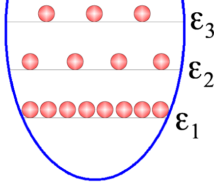
Figure 1: Scheme of the Bose-Einstein condensation of trapped atoms

Suppose that a system of many atoms is confined in a trapping potential, with a discrete energy spectrum characterized by the level energies $\varepsilon_{1},\varepsilon_{2},\ldots,\varepsilon_{n},\ldots$. Atoms are distributed over these energy levels, so as to achieve the minimal free energy for the system. At sufficiently low temperature, a great number of atoms pile down in the lowest energy level, as shown in Fig. 1. This concentration of atoms in the lowest level is the Bose-Einstein condensation. While the lowest level corresponds to the minimal energy, not all atoms are able to occupy it, and there are always atoms on other higher energy levels. This corresponds to the condensate depletion that is caused by two reasons: temperature fluctuations and repulsive atomic interactions. In the presence of the Bose condensate, the distribution of atoms over energy levels cannot be given by a single function, but the condensate has to be separated out from the distribution of the rest of the atoms. Consequently, the condensate is nothing but a statistical outlier.

A similar phenomenon occurs in a statistical system of agents that can occupy different“levels” corresponding to different ranks, such as the inhabitants of different cities. And each given country is finite, similarly to a finite system of trapped atoms. Discrete energy levels are analogous to separate cities. People tend to live in those cities that are the most convenient and profitable for them. Usually, the best opportunities are provided by the largest cities classified by the lowest ranks, within a rank-ordering classification. Thus, the largest city can become an outlier, if a Bose-Einstein condensation occurs. And similarly to the case of atoms, not all people can gather in a single city because of various disturbing factors and individual competitive interactions. The concentration of people in the largest city is equivalent to the Bose condensation. Then, the distribution of inhabitants over all cities can describe all the cities at the exception of the city-outlier that has to be separated from the distribution, in the same way as it is done for a Bose-condensed system of atoms.

The Bose-Einstein condensation of atoms results from the Bose statistics that is at the origin of correlations between atom occupancies over the population of available energy levels. Analogously, the correlations among people are realized by the exchange of information. The choice of cities and the evaluation of their suitability, or fitness, or attractiveness, is always done on the basis of the information available to decision makers. The information exchange between people plays the role of quantum correlations for atoms.

Information processing, of course, requires time and can depend on the geometric location of participants, similarly to the processes of atomic interactions. The time scaled involved in information exchange is much shorter than the typical lifetime of a country. This is in analogy with the smallness of the atomic interaction time as compared with the lifetime of a trapped system. Therefore, it is admissible to invoke an equilibrium description, where the short time-dependent processes are averaged out. As a result, such an equilibrium description does not depend on time and on the spatial location of participants.

In order to summarize the analogies between the Bose-Einstein condensation of trapped atoms and the condensation of inhabitants in cities, we give below a dictionary connecting these phenomena.

confining potential	country territory
trapped atoms	country citizens
energy levels	separate cities
level number	city rank
level distribution	rank distribution
quantum correlations	information exchange
thermal fluctuations	disturbing factors
repulsive interactions	competitive interactions
energy minimization	utility maximization
most profitable level	most profitable city

2.2 Definitions and formulation of the model

Our approach is general, being applicable to various statistical data. For the sake of concreteness, we illustrate it for the case of the rank-size distribution of cities in a country. Equally, the approach is valid for the rank-frequency distribution of words in a text, as well as for other statistical data in sociology, linguistics, economics, and so on.

We consider the situation when the process of city formation has reached a stationary regime inside the given country [61]. This condition holds by construction in the case of the word-frequency distribution in a given text, which is written and therefore fixed.

Let $N$ be the total number of persons (or households or other atomic groups) representing the total population of a country. Or this could be the total number of words in a text. This means that the population can be grouped into characteristic population elements indexed by $n=1,2,\ldots,N$. Or this could be the number of word groups, each group consisting of the same word. The total number $N$ is assumed to be very large, $N\gg 1$. This population of $N$ persons is distributed among $C$ cities.

The city rank $\varepsilon(n)$ of a city with $n$ inhabitants is defined as the number of cities whose population is larger than or equal to $n$ inhabitants. This means that the rank is related to the cumulative distribution of population over cities. The ranks are arranged in the ascending order, so that the rank of a larger city is smaller:

$$\varepsilon(n_{1})<\varepsilon(n_{2})\qquad(n_{1}>n_{2})\;.$$ (1)

Rank $1$ corresponds to the largest city, rank $2$ to the second largest city, and so on. Our aim is to find a relation between the city rank and its characteristic population.

The relation and our derivation of the Bose-Einstein condensation phenomenon in the distribution of cities relies on three key ingredients.

Assumption 1. The characteristic feature of an inhabitant selecting a city can be described by the concept of utility factor $w(\varepsilon)$, which is assumed to be a function only of the city rank $\varepsilon$.

Justification. Each city has evolved during its history, in competition and through diverse complex interactions with other cities in the country. The characteristic feature of an inhabitant selecting a city can be described by the factor $w(\varepsilon)$ characterizing the stationarity state of the relative attraction, according to the usefulness for the decision maker, of each of the $C$ cities to the diverse individuals in the total population of $N$ persons. The utility factor $w(\varepsilon)$ takes the values within the interval $[0,1]$; the larger its numerical value, the more convenient and the more attractive is the city. The factor $w(\varepsilon)$ is a decreasing function of rank $\varepsilon$.

Assumption 2. The attraction factor $w(\varepsilon)$ is taken to be an exponentially decreasing function of rank:

$$w(\varepsilon)=be^{-\beta\varepsilon}\qquad(b>0\;,\;\beta>0)\;.$$ (2)

Justification. This is a natural choice, very often assumed in the biological literature dealing with fitness [62-71]. The parameter $\beta$ is called the decline parameter. The fitness factor decreases with rank, capturing the fact that a smaller city (higher rank) is less attractive, in general, due to less opportunities for job, cultural entertainments, synergies and so on [72]. The attraction of large cities is usually associated with increasing returns to scale and economies of scale [73]. The utility function in decision theory is also often taken in the exponential form [74,75].

Assumption 3. The probability that a city of rank $\varepsilon$ has a population of not less than $n$ inhabitants is assumed to be a multiplicative function of the utility factors for each person:

$$p_{n}(\varepsilon)=aw^{n}(\varepsilon)\;.$$ (3)

Justification. This expression (3) derives from the assumption that separate individuals make their choices independently from each other. As the overall quality or attraction of a city for a given person is completely captured by the utility factor $w(\varepsilon)$, the population of a given city then results from independent choices performed by each inhabitant, which is equivalent to taking the product of the factors $w(\varepsilon)$.

3 Derivation of the rank-size cumulative distribution

The probability $p_{n}(\varepsilon)$ given by (3) has to be normalized as

$$\sum_{n=1}^{N}p_{n}(\varepsilon)=1\;,$$ (4)

in order to express that each city is certainly inhabited. This normalization, taking into account that

$$\sum_{n=1}^{N}w^{n}\simeq\frac{w}{1-w}\qquad(N\gg 1)\;,$$

yields

$$a=\frac{1-w}{w}\;.$$

Therefore, the probability $p_{n}(\varepsilon)$ defined by (3) acquires the form

$$p_{n}(\varepsilon)=[1-w(\varepsilon)]w^{n-1}(\varepsilon)\;.$$ (5)

The characteristic population of a city of rank $\varepsilon$ is defined as the expectation value

$$n(\varepsilon)=\sum_{n=1}^{N}np_{n}(\varepsilon)\;.$$ (6)

This, in view of the equality

$$\sum_{n=1}^{N}nw^{n}\simeq\frac{w}{(1-w)^{2}}\qquad(N\gg 1)\;,$$

gives the expression

$$n(\varepsilon)=\frac{1}{1-w(\varepsilon)}\;.$$ (7)

Expression (7) is valid for any type of attraction factor $w(\varepsilon)$. Generally, the latter could be taken in different forms, but here we employ the expression (2).

With the form (2) of the attraction factor, the characteristic population (7) becomes

$$n(\varepsilon)=\frac{e^{-\beta\varepsilon}}{e^{\beta\varepsilon}-b}\;.$$ (8)

Introducing the notation

$$\mu\equiv\frac{1}{\beta}\;\ln b$$ (9)

reduces Eq. (8) to

$$n(\varepsilon)=\frac{e^{\beta(\varepsilon-\mu)}}{e^{\beta(\varepsilon-\mu)}-1}\;.$$ (10)

This has the form of the typical Bose-Einstein function describing the population distribution, with the nominator playing the role of a degeneracy factor, the rank $\varepsilon$ playing the role of energy, and $\mu$ playing the role of a chemical potential.

Inverting Eq. (10) gives the rank of a given city

$$\varepsilon(n)=\mu+\frac{1}{\beta}\;\ln\left(\frac{n}{n-1}\right)$$ (11)

as a function of its characteristic population size $n$. A priori, the rank cannot be smaller than one for all population sizes $n$ larger than one:

$$\varepsilon(n)\geq 1\qquad(n>1)\;.$$ (12)

In this way, Eq. (10) gives the expectation value of the population size for a city of rank $\varepsilon$. Here the rank is fixed. Equation. (11), conversely, defines the rank for the given characteristic population size. Recall that $n(\varepsilon)$ is a cumulative distribution, hence its sum over the ranks does not define the total country population.

The formal definition of a city is a disputed and complex issue, that we do not address here. Let us just mention that cities have more than one inhabitant, being relatively large and permanent settlements, with administrative, legal, or historical status based on local law. Thus, there should be in general one more restriction on the rank, when the lowest characteristic population is fixed by some number $m$, so that all $C$ cities have populations not smaller than this minimal number $m$. Then the boundary condition follows:

$$\varepsilon(m)=C\;,$$ (13)

which defines the chemical potential

$$\mu=C-\;\frac{1}{\beta}\;\ln\left(\frac{m}{m-1}\right)\;.$$ (14)

Expression (11) retrieves a variant of Zipf’s law for the largest cities. Indeed, taking $n\gg 1$ allows one to expand the logarithm and obtain

$$\varepsilon(n)=\mu+\frac{1}{\beta}\cdot\frac{1}{n}\qquad(n\gg 1)\;,$$ (15)

relating the city rank to the inverse of the population size. The only difference with the standard formulation of Zipf’s law is the term $\mu$ that gives a small correction. Since $n(\varepsilon)$, by definition, is positive, then $\mu$ should be smaller than the minimal $\varepsilon$ equal to one. Hence $\mu<1$.

4 Bose-Einstein condensation into dragon-king cities

It turns out that the distributions (10) and (15) are not the whole story. Indeed, the boundary condition (13) may sometimes disagree with the population distribution (10). The occurrence of such a disagreement signifies the appearance of an anomaly, that we term a “dragon-king” city [34], which is equivalent to Bose-Einstein condensation.

To demonstrate how this happens, let us consider the population of the most inhabited city of rank one

$$N_{1}\equiv n(1)=\frac{e^{\beta(1-\mu)}}{e^{\beta(1-\mu)}-1}\;.$$ (16)

By its definition, this is a finite positive number, which requires that $\mu$ be smaller than one,

$$\mu<1\qquad(0<N_{1}<\infty)\;.$$ (17)

The latter implies that the decline parameter $\beta$ has to be limited by the inequality

$$\beta<\beta_{c}\qquad(\mu<1)\;,$$ (18)

where the critical value is defined by

$$\beta_{c}\equiv\frac{1}{C-1}\;\ln\left(\frac{m}{m-1}\right)\;.$$ (19)

When condition (18) holds true, the boundary condition (13) is compatible with the population distribution (10). Therefore, the rank-size distribution of cities follows formula (11) with $\mu$ given by equality (14).

However, when $\beta$ becomes larger than the critical value $\beta_{c}$, the boundary condition (13) becomes incompatible with the population distribution (10). A large value of $\beta$ implies a relatively much stronger attraction to the first rank compared with the higher ranks. It is therefore expected that the largest city, rank $1$, plays a special role. Indeed, considering that the largest city of rank $1$ is an outlier of the distribution of all other cities, that we refer to as a dragon-king, we should exclude it from the statistics described by distribution (11). The remaining cities continue to be described by this distribution. The situation is completely analogous to the Bose-Einstein condensation, where the role of the dragon-king is played by the Bose condensate. In that sense, the dragon-king represents a condensate droplet, with its inhabitants playing the role of condensate particles.

In general, it is possible that several largest cities could be outliers (dragon-kings) of the distribution of city sizes and thus should be excluded from the description offered by formula (11). In physics, this would correspond to the occurrence of granular condensate consisting of several grains, or droplets, of condensed particles in the surrounding of uncondensed matter [52,76]. For instance, if $k$ cities are dragon-kings, then for the population $n(k)$ to be a positive number, $\mu$ has to be smaller than $k$, hence the decline parameter $\beta$ has to be constrained by the inequality

$$\beta<\frac{1}{C-k}\;\ln\left(\frac{m}{m-1}\right)\;.$$ (20)

In that case, a series of condensation transitions would arise, with the condensation of the largest city, then of the second largest one, and so on as the decline factor $\beta$ increases through the succession of the critical values, corresponding to a larger and larger mismatch between the attraction factors of large cities and smaller ones.

For the convenience of presenting the formulas, let us introduce the parameter that can be called the effective temperature

$$T\equiv\frac{\beta_{c}}{\beta}\;.$$ (21)

This parameter quantifies the level of noise causing the dispersion of the country inhabitants among different cities. Then the rank-size distribution (11) takes the form

$$\varepsilon(n)=\mu+\frac{T}{\beta_{c}}\;\ln\left(\frac{n}{n-1}\right)\;,$$ (22)

with the chemical potential

$$\mu=C-(C-1)T\;.$$ (23)

For high temperature $T>1$, one has $\mu<1$, and there is no condensation. The value $T_{c}=1$ is the critical point of the starting condensation, where $\mu=1$. Below this temperature $T<1$, the largest city of rank $1$ falls out of the data sample, becoming a dragon-king, with other cities remaining uncondensed and described by the rank-size distribution (11).

With these notations, the generalized Zipf’s law, obtained for large $n$, reads as

$$\varepsilon\simeq\mu+\left(\frac{T}{\beta_{c}}\right)\frac{1}{n}\qquad(n\gg 1~{}~{}~{}\&~{}~{}~{}\mu<1)~{},$$ (24)

relating the rank $\varepsilon$ of a given city to its population size $n$. In this way, our model not only gives the interpretation of outliers in the distribution of city sizes as Bose-condensed droplets, but it also provides a possible mechanism for the Zipf’s law.

5 Discussion

We have suggested a novel approach for deriving rank-size distributions. First, we obtain the Zipf law that has been well documented for a variety of statistical data. Secondly, according to this approach, the appearance of outliers of the distributions, that we have referred to as “dragon-kings” [34], is equivalent to the Bose-Einstein condensation. The objects of the first ranks, such as the largest cities, when becoming outliers, are similar to Bose-condensed droplets. For concreteness, we followed the interpretation related to the rank-size distribution of cities. But the approach can be applied for interpreting the appearance of outliers of other nature, e.g., in the rank-frequency distribution of words in different texts.

In physics, the Bose-Einstein condensation is a collective coherent phenomenon. The same interpretation applies to our derivation through the three assumptions underlying our model, which are set to capture the collective organization of cities over their historical development. Consequently, the appearance of dragon-kings can also be understood as the result of collective effects resulting in the coherent accumulation of agents in these outliers. The Bose condensation is a phase transition. Hence, we propose that the occurrence of “dragon-kings” [34] is also a kind of a phase transition. Other related mechanisms for the formation of dragon-kings are also associated with phase transitions. Let us mention generalized percolation transition, where the infinite cluster plays the role of the outlier or dragon-king. Another example is that of the synchronization between moving objects, like oscillators [77], which can give rise to the coexistence of a power law distribution of event sizes and of dragon-kings [78-80].

When dealing with statistical data, there are phenomenological recipes that allow one to suspect the presence of outliers [1-3]. The simplest hint that the object of rank $1$ is an outliers is when

$$n(1)-n(2)\gg n(2)-n(3)\;.$$ (25)

In the approach we suggest, the procedure would be as follows. For the given numbers $m$ (of a minimum city size) and $C$ (number of cities in the country) characterizing the considered statistical set, one should fit the function $\varepsilon(n)$ to the given data, thus, defining the parameter $T$. One should compare the fittings with and without the object suspected to be an outlier. Comparing these fittings and the related values of $T$ and $\mu$, one could conclude, in line with the above theory, whether there is condensation or not. Condensation should correspond to the low temperature $T<1$.

The suggested method of describing outliers applies to the sets of given data, such as city sizes or word frequencies. One could ask the question whether the method could be transferred to systems with time evolution, such as stock market data accompanied by crashes? The principal answer to this question is yes, provided the whole set of data is given. Omitting details, the idea for using the method to temporal data would be as follows. Let a database of time series be given, where one can define the drawdowns, occurring at different times and quantified by some index. And let $n$ be the value measuring the fall of the index from some previous peak value. Suppose $\varepsilon(n)$ is the number of drawdowns whose fall index is larger than $n$. This $\varepsilon(n)$ plays the role of the drawdown rank. Then we may follow the general consideration described above. The largest drawdown becomes an outlier when condensation occurs. Then this condensed outlier represents a market crash.

The aim of the present paper has been the development of a general theory. So, here we limit ourselves by the principal points. Applications to particular examples involve discussions of technical problems of fitting methods, which is out of the scope of the present paper. Different applications will be treated in separate publications.

References

- [1] F.E. Grubbs, Technometrics 11, 1-21 (1969).
- [2] V. Barnett, T. Lewis, Outliers in Statistical Data (Wiley, New York, 1994).
- [3] P. Rousseeuw, A. Leroy, Robust Regression and Outlier Detection (Wiley, New York, 1996).
- [4] V. Pareto, Cours d’Economie Politique (Droz, Geneva, 1896).
- [5] J.B. Estoup, Gammes Stenographiques (Institut Stenographique de France, Paris, 1916).
- [6] J.C. Willis, Age and Area (Cambridge University, Cambridge, 1922).
- [7] G.U. Yule, Statistical Study of Literary Vocabulary (Cambridge Univesrity, Cambridge, 1944).
- [8] G.K. Zipf, Human Behavior and the Principle of Least Effort (Addison-Wesley, New York, 1949).
- [9] B.B. Mandelbrot, Compt. Rend., 232, 1638-1640 (1951).
- [10] B.B. Mandelbrot, Compt. Rend., 232, 2003-2005 (1951).
- [11] G.A. Milller, Annu. Rev. Psychol., 5, 401-420 (1954).
- [12] L. Egghe, R. Rousseau, Introduction to Informetrics: Quantitative Methods in Library, Documentation and Information Science (Elsevier, Amsterdam, 1990).
- [13] J. Nicolis, Chaos and Information Processing: A Heuristic Outline (World Scientific, Singapore, 1991).
- [14] A. Miller, The Science of Words (Freeman, New York, 1991).
- [15] H.A. Simon, Biometrika 42, 425-440 (1995).
- [16] P. Krugman, The Self-Organizing Economy (Blackwell, Cambridge, 1996).
- [17] D. Sornette, L. Knopoff, Y.Y. Kagan, C. Vanneste, J. Geophys. Res., 101, 13883-13894 (1996).
- [18] B.B. Mandelbrot, Fractals and Scaling in Finance : Discontinuity, Concentration, Risk (Springer, Berlin, 1997).
- [19] D. Sornette, D. Zajdenweber, Eur. Phys. J. B, 8, 653-664 (1998).
- [20] J.P. Bouchaud, D. Sornette, C. Walter, J.P. Aguilar, Int. J. Theor. Appl. Finance 1, 25-41 (1998).
- [21] M.A. Nowak, J. Theor. Biol. 204, 179-189 (2000).
- [22] A. Johansen, D. Sornette, Physica A 276, 338-345 (2000).
- [23] P. Harremoees, F. Topsoe, Entropy 3, 227-292 (2001).
- [24] J. Camacho, R.V. Sole, Eur. Phys. Lett. 55, 774-780 (2001).
- [25] W. Li, Y. Yang, J. Theor. Biol. 219, 539-551 (2002).
- [26] D. Sornette, Why Stock Markets Crash (Princeton University, Princeton, 2003).
- [27] J. Eeckhout, Am. Econom. Rev. 94, 1429-1451 (2004).
- [28] R. Suzuki, J.R. Buck, P.L. Tyacks, Animal Behav. 69, 9-17 (2005).
- [29] C. Anderson, Long Tail. Why the Future of Business is Selling Less of More (Hyperion, New York, 2006).
- [30] A. Clauset, C.R. Shalazi, M.E. Newman, SIAM Rev. 51, 661-703 (2009).
- [31] M. Levy, Am. Econom. Rev. 99, 1672-1675 (2009).
- [32] A. Saichev, Y. Malevergne, D. Sornette Theory of Zipf’s Law and Beyond (Springer, Berlin, 2009).
- [33] World Gazetteer Database (2010).
- [34] D. Sornette, Int. J. Terraspace Sci. Eng. 2, 1-18 (2009).
- [35] N.N. Taleb, The Black Swan (Penguin, Harlow, 2010).
- [36] J.I. Frenkel, Kinetic Theory of Liquids (Clarendon, Oxford, 1946).
- [37] D. ter Haar, Elements of Statistical Mechanics (Rinehart, New York, 1954).
- [38] M.E. Fisher, Nature of Critical Points (Colorado University, Boulder, 1965).
- [39] M.E. Fisher, Rep. Prog. Phys. 30, 615-730 (1967).
- [40] K. Binder, D. Stauffer, Adv. Phys. 25, 343-396 (1976).
- [41] V.I. Yukalov, Phys. Rep. 208, 395-489 (1991).
- [42] P. Bialas, Z. Burda, D. Johnston, Nucl. Phys. B 542, 413-424 (1999).
- [43] V.I. Yukalov, E.P. Yukalova, Physica A 243, 382-414 (1997).
- [44] V.I. Yukalov, E.P. Yukalova, Phys. Part. Nucl. 28, 37-65 (1997).
- [45] M. Marsili, Y.C. Zhang, Phys. Rev. Lett. 80, 2741-2744 (1998).
- [46] J.O. Andersen, Rev. Mod. Phys. 76, 599-639 (2004).
- [47] V.I. Yukalov, Laser Phys. Lett. 1, 435-461 (2004).
- [48] V.I. Yukalov, D. Girardeau, Laser Phys. Lett. 2, 375-382 (2005).
- [49] A. Posazhennikova, Rev. Mod. Phys. 78, 1111-1134 (2006).
- [50] V.I. Yukalov, Laser Phys. Lett. 4, 632-647 (2007).
- [51] N.P. Proukakis, B. Jackson. J. Phys. B 41, 203002 (2008).
- [52] V.I. Yukalov, Laser Phys. 19, 1-110 (2009).
- [53] V.I. Yukalov, Phys. Part. Nucl. 42, 460-513 (2011).
- [54] H. Frohlich, Int. J. Quant. Chem. 2, 641-649 (1968).
- [55] J. Pascual-Leone, Acta Psychol. 32, 301-345 (1970).
- [56] V. Weiss, H. Weiss, Chaos Solit. Fract. 18, 643-652 (2003).
- [57] M.R. Evans, T. Hanney, J. Phys. A 38, 195-239 (2005).
- [58] J.P. Bouchaud, M. Mezard, Physica A 282, 536-545 (2000).
- [59] G. Bianconi, A.L. Barabasi, Phys. Rev. Lett. 86, 5632-5635 (2001).
- [60] G. Bianconi, L. Ferretti, S. Franz, Eur. Phys. Lett. 87, 28001 (2009).
- [61] W. Weidlich, Phys. Rep. 204, 1-163 (1991).
- [62] B.F. Manly, Heredity 36, 229-234 (1976).
- [63] R.H. Crozier, P. Pamilo, Austral. J. Biol. Sci. 32, 469-474 (1979).
- [64] I.S. Novella, E.A. Duarte, S.F. Elena, A. Moya, E. Domingo, J.J. Holland, Proc. Natl. Acad. Sci. USA 92, 5841-5844 (1995).
- [65] D.A. Russell, Geol. Soc. Am. 307, 381-388 (1996).
- [66] A. Arias, E. Lazaro, C. Escarmis, E. Domingo, J. Gen. Virol. 82, 1049-1060 (2001).
- [67] G. Palyi, C. Zucchi, L. Caglioty, eds., Progress in Biological Chirality (Elsevier, Amsterdam, 2004).
- [68] M.C. Cowperthwaite, J.J. Bull, L.A. Meyers, Genetics 170, 1449-1457 (2005).
- [69] S. Bershtein, M. Segal, R. Bekerman, N. Tokuriki, D.S. Tawlih, Nature 444, 929-932 (2006).
- [70] G. Martin, T. Lenormand, Genetics 179, 907-916 (2008).
- [71] D.B. Saakian, A.S. Martirosyan, C.K. Hu, Phys. Rev. E 81, 061913 (2010).
- [72] L.M.A. Bettencourt, J. Lobo, D. Helbing, C. Kühnert, G.B. West, Proc. Natl. Acad. Sci. USA 104, 7301-7306 (2007).
- [73] B. O’Flaherty, City Economics (Harvard University, Cambridge, 2005).
- [74] P. Weirich, Decision Space (Cambridge University, Cambridge, 2000).
- [75] C. Gollier, Economics of Risk and Time (MIT, Cambridge, 2001).
- [76] V.I. Yukalov, E.P. Yukalova, V.S. Bagnato, Laser Phys. 19, 686-699 (2009).
- [77] V.I. Yukalov, Coherence phenomena, in Encyclopedia of Nonlinear Science, ed. A. Scott (Routledge, New York, 2005), p. 144-147.
- [78] L. Gil, D. Sornette, Phys. Rev. Lett. 76, 3991-3994 (1996).
- [79] I. Osorio, M.G. Frei, D. Sornette, J. Milton, Y.C. Lai, Phys. Rev. E 82, 021919 (2010).
- [80] D. Sornette and I. Osorio, “Prediction”, in: Epilepsy: The Intersection of Neurosciences, Biology, Mathematics, Physics and Engineering, eds. I. Osorio, H.P. Zaveri, M.G. Frei, S. Arthurs (Taylor and Francis, London, 2010), p. 203-237.