Squirals and beyond: Substitution tilings
with singular continuous spectrum

Abstract.

The squiral inflation rule is equivalent to a bijective block substitution rule and leads to an interesting lattice dynamical system under the action of $\mathbb{Z}^{2}$. In particular, its balanced version has purely singular continuous diffraction. The dynamical spectrum is of mixed type, with pure point and singular continuous components. We present a constructive proof that admits a generalisation to bijective block substitutions of trivial height on $\mathbb{Z}^{d}$.

1. Introduction

Dynamical systems of translation bounded measures on $\mathbb{R}\hskip 0.5pt^{d}$ with pure point spectrum are well understood by now. This owes a lot to the equivalence between pure point dynamical and diffraction spectra [33, 11], and to the general characterisation of model sets via dynamical systems; see [12] and references therein. From an applied perspective, pure point spectra are linked to the analysis of periodic and almost periodic systems, such as crystals and quasicrystals, by standard crystallographic methods; see [18] for background, and [10] for a recent review in the aperiodic setting. In fact, the understanding of pure point systems has improved sufficiently that one can begin to attack the corresponding inverse problem systematically [35].

As soon as one enters the realm of mixed spectra, the picture is less transparent. While some partial understanding exists for systems with absolutely continuous spectral components (for instance through the connection with the highly developed field of stochastic processes; see [5] and references therein), one is pretty much in the dark when it comes to systems with singular continuous spectra. The classic Thue-Morse system, see [2] for background, and its generalisations in the spirit of [30, 6] are notable exceptions, which are all one-dimensional.

Beyond the theoretical interest, there was little motivation in the past to dive further into systems with continuous spectral components, at least not from an applied point of view. However, with the modern measurements possible in materials science, spectra of this type are detectable and observed more frequently [48], so that some further analysis is needed. One obstacle has been that practically no examples in higher dimensions are known, and certainly not in an explicit fashion. This, in turn, is where the classic Thue-Morse system excels: Since its original (spectral) discussion in [47, 36] and its later reformulation in [28], it has been the paradigm of singular continuous (dynamical) spectrum, and it is actually rather easy to also calculate its distribution function explicitly and with high precision; see [8] and references therein for details and [49] for an approach to the analysis of its ‘fractal’ aspects. The good accessibility of the latter is a consequence of the underlying Riesz product structure; see [50] for background material.

However, the situation is not as bad as it appears. A substantial step forward was achieved in [32, 33, 34] for lattice substitution systems by identifying modular coincidence as one viable and powerful generalisation of Dekking’s criterion [19] for pure pointedness in one-dimensional substitutions of constant length. The interesting cases are the systems that fail to possess a modular coincidence, such as the bijective substitutions of constant length and their higher-dimensional generalisations studied in [20, 21]. However, to the best of our knowledge, no serious attempt has been made to investigate a genuinely higher-dimensional example with singular continuous spectrum explicitly (by which we mean an example that cannot be written as a product of one-dimensional systems, such as those appearing in [26]).

Here, we report on a planar example that was identified as a good candidate in [22], and could be tackled with the methods explained in [23]. It it known as the squiral tiling and appears in [25, Fig. 10.1.4], where it was constructed as a simple example for a tiling of the plane by one prototile with infinitely many edges (and its mirror image). It is obtained by means of the simple inflation rule

(1)

together with the corresponding rule for the opposite chirality of the squiral prototile. It has the integer inflation multiplier $3$ and defines an aperiodic tiling of the Euclidean plane. The term ‘aperiodicity’ is used in its strong version here, hence meaning that the inflation rule defines a unique hull (via the closure of the $\mathbb{Z}^{2}$-orbit of a fixed point in the local topology) with the property that no element of this hull admits a non-trivial period. A larger patch of the tiling is shown in Figure 1.

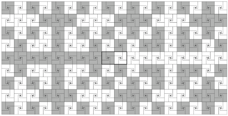
Figure 1. A rectangular patch of the squiral tiling with a ‘black and white’ reflection symmetry in the vertical axis. The displayed patch was obtained via two inflation steps of (1) from the central rectangular seed (marked), the latter comprising four tiles of each chirality.

As an application of [23], Frettlöh and Sing checked that this tiling has no modular coincidence, so cannot be a model set, wherefore this is a candidate for a mixed spectrum. In what follows, we reformulate this tiling via a topologically conjugate one (by mutual local derivability [15, 3]) and bring it to the simpler setting of block or lattice substitutions. It will then be possible to show that its balanced version (with weights $1$ and $\bar{1}=-1$ of equal frequency) has purely singular continuous diffraction spectrum. As a consequence, the dynamical spectrum will be a mixture of a pure point and a singular continuous part, in line with the (implicit) conjecture in [20].

Our approach (as indicated already) will be constructive, so that we do not only determine the spectral type, but also derive the diffraction measure explicitly. In fact, we can identify it as a two-dimensional Riesz product. This means that one can formulate a simple recursion for a sequence of 2D continuous distribution functions that converge towards the distribution function of the squiral measure, and uniformly so (even though the underlying measures are absolutely continuous, and can thus only converge to the squiral measure in the vague topology).

In Section 7, this approach is generalised to primitive and bijective block substitutions of constant length over a binary alphabet, in arbitrary dimension $d$. We prove that these systems show singular continuous diffraction if the height lattice is trivial.

2. Squirals and lattice inflations

The squiral inflation of Eq. (1) is primitive, with inflation matrix $M=\left(\begin{smallmatrix}5&4\\ 4&5\end{smallmatrix}\right)$. The latter has eigenvalues $9=3^{2}$ and $1$, with Perron-Frobenius eigenvector $(1,1)$, which is in line with both chiralities occupying the same area and occurring with equal frequency (via reading it as left or as right eigenvector). Moreover, if we add one pseudo-vertex at the middle of the long edge of the squiral, the inflation tiling is face to face as well. As such, it defines a strictly ergodic dynamical system under the shift action of $\mathbb{Z}^{2}$. Note that the special (spiralling) vertex always falls on the centre of a square that is formed by $4$ squirals of the same chirality. This also explains the name as a mixture of ‘square’ and ‘spiral’. It is natural to view the squiral tilings as a (local) decoration of the square lattice, where the colour simply codes the chirality of the square decoration. This correspondence gives rise to a mutually local rule in the sense of [15, 3] as follows.

The first step consists of identifying an induced inflation rule on the coloured square lattice, which is simply given by

(2)

This defines a block substitution that is bijective and of constant length in the terminology of [20]. As a coloured tiling, it is thus defined by a primitive inflation rule (with the same inflation matrix $M$ as before). One quickly checks that the inflation action and the derivation rule (now applicable in either direction) commute, so that the block substitution defines a hull that is mutually locally derivable (MLD) to the squiral hull. It is clear that the former is better suited for our further analysis.

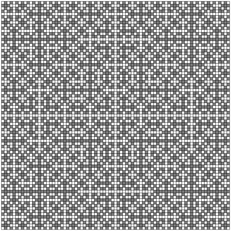
Figure 2. A square-shaped patch of the squiral tiling with full $D_{4}$-symmetry, as obtained from the equivalent block substitution (2).

If one iterates the block substitution starting from a single square with its centre as reference point, one obtains a sequence of growing (finite) tilings that converges to a tiling of the plane which is a fixed point; see Figure 2 for an illustration. This particular tiling has perfect $D_{4}$-symmetry and defines (via its hull, the closure of its $\mathbb{Z}^{2}$-orbit in the local topology) a minimal dynamical system that is uniquely ergodic. This follows from standard arguments because the inflation is primitive and leads to a face to face tiling of finite local complexity. As a consequence, the fixed point is linearly repetitive, which implies the claim by [31, Thm. 6.1]. For some general results on tiling dynamical systems, we refer to [41, 44, 20].

3. Autocorrelation coefficients

Let us now represent each (coloured) square by a point at its lower left corner that carries a matching colour, which we call $1$ (for white) or $\bar{1}$ (for grey). The hull $\mathbb{X}$ is then a closed subspace of $\{1,\bar{1}\}^{\mathbb{Z}^{2}}$ that is invariant under the shift action of $\mathbb{Z}^{2}$ by construction. Given $w\in\mathbb{X}$, we define the corresponding Dirac comb

(3) $$\omega\,=\,w\hskip 0.5pt\delta_{\mathbb{Z}^{2}}\,=\sum_{z\in\mathbb{Z}^{2}}w_{z}\hskip 0.5pt\delta_{z}\hskip 0.5pt,$$

where we write $z\in\mathbb{Z}^{2}$ as a pair of integers from now on. For the weights, we use the convention $\bar{1}=-1$. Following the approach pioneered by Hof [27], we define the natural autocorrelation measure $\gamma$ of $\omega$ as

(4) $$\gamma\,=\,\omega\circledast\widetilde{\omega}\,:=\,\lim_{N\to\infty}\frac{\omega\big{|}_{C_{N}}\!*\,\widetilde{\omega\big{|}_{C_{N}}}}{(2N+1)^{2}}$$

where $C_{N}$ denotes the closed centred square of side length $2N$. Here, $\widetilde{\mu}$ denotes the measure defined by $\widetilde{\mu}(g)=\overline{\mu(\widetilde{g})}$ for $g\in C_{\mathsf{c}}(\mathbb{R}\hskip 0.5pt^{2})$, with $\widetilde{g}(x):=\overline{g(x)}$. The limit in Eq. (4) always exists due to unique ergodicity, and is independent of the choice of $w\in\mathbb{X}$. The measure $\gamma$ is of the form $\gamma=\eta\hskip 0.5pt\hskip 0.5pt\delta_{\mathbb{Z}^{2}}$ with coefficients

$$\eta\hskip 0.5pt(m,n)\,=\,\lim_{N\to\infty}\frac{1}{(2N+1)^{2}}\sum_{k,\ell=-N}^{N}w_{k,\ell}\,w_{k-m,\ell-n}\hskip 0.5pt,$$

where the result is again independent of the choice of $w$. We discuss the convergence of these sums in more detail later.

Due to the symmetry of our system, it suffices to consider the positive quadrant and formulate the autocorrelation accordingly. This simplifies our further calculations. To this end, we consider the square inflation with the lower left corner as new reference point, and observe that this, when starting from a single block, leads an iteration sequence which fills the positive quadrant only. To obtain a complete tiling, one may start from the legal seed $\begin{smallmatrix}\bar{1}&1\\ 1&\bar{1}\end{smallmatrix}$ with reference point in its centre. Recall that a patch is called legal when it occurs in the $n$-fold substitution of a single letter, for some $n\in\mathbb{N}$. The iteration of the substitution then converges towards a $2$-cycle that covers $\mathbb{Z}^{2}$, each element of which defines the same hull. The substitution is still a $2$-cycle when restricted to the positive quadrant. Due to the $D_{4}$-symmetry of the pattern in Figure 2, and hence that of the entire hull $\mathbb{X}$, it is sufficient to calculate the autocorrelation coefficients within the positive quadrant.

Denote the two configurations in the positive quadrant (written in the alphabet $\{1,\bar{1}\}$, with $\bar{\bar{1}}=1$) by $v$ and $\varrho v$. They satisfy

(5) $$(\varrho v)_{3m+r,3n+s}\,=\,\begin{cases}\overline{v}_{m,n},&\text{if }r\equiv s\equiv 0\bmod 2,\\ v_{m,n},&\text{otherwise},\end{cases}$$

where $m,n\geq 0$ and $0\leq r,s\leq 2$. The autocorrelation coefficients clearly satisfy

(6) $$\eta\hskip 0.5pt(m,n)\,=\lim_{N\to\infty}\frac{1}{N^{2}}\sum_{k,\ell=0}^{N-1}(\varrho v)_{k,\ell}\,(\varrho v)_{k+m,\ell+n}\,=\lim_{N\to\infty}\frac{1}{N^{2}}\sum_{k,\ell=0}^{N-1}v_{k,\ell}\,v_{k+m,\ell+n}$$

for $m,n\geq 0$. All limits exist due to unique ergodicity and the fact that the sum is an orbit average of a continuous function [46]. Moreover, we have used the symmetry to write $\eta$ via the positive quadrant only. Clearly, we have $\eta\hskip 0.5pt(0,0)=1$ together with

(7) $$\eta\hskip 0.5pt(-m,n)\,=\,\eta\hskip 0.5pt(m,-n)\,=\,\eta\hskip 0.5pt(-m,-n)\,=\,\eta\hskip 0.5pt(m,n)\hskip 0.5pt,$$

which specifies the function $\eta$ on all of $\mathbb{Z}^{2}$. Note that the $D_{4}$-symmetry of our system also implies the relation $\eta\hskip 0.5pt(m,n)=\eta\hskip 0.5pt(n,m)$.

For our further analysis, we introduce the shorthand

$$\langle m,n\rangle\,:=\,\eta\hskip 0.5pt(m,n)\hskip 0.5pt.$$

Considering the coefficient $\langle 3m\!+\!r,3n\!+\!s\rangle$ for $\varrho v$ and fixed $m,n\geq 0$ and $0\leq r,s\leq 2$, one can split the defining sum modulo $3$ and use Eqs. (5) and (6) to derive the recursion relations

(8) $$\begin{split}\langle 3m,3n\rangle\,&=\,\langle m,n\rangle\\ \langle 3m,3n\!+\!1\rangle\,&=\,-\tfrac{2}{9}\langle m,n\rangle+\tfrac{1}{3}\langle m,n\!+\!1\rangle\\ \langle 3m,3n\!+\!2\rangle\,&=\,\tfrac{1}{3}\langle m,n\rangle-\tfrac{2}{9}\langle m,n\!+\!1\rangle\\[2.84526pt] \langle 3m\!+\!1,3n\rangle\,&=\,-\tfrac{2}{9}\langle m,n\rangle+\tfrac{1}{3}\langle m\!+\!1,n\rangle\\ \langle 3m\!+\!1,3n\!+\!1\rangle\,&=\,-\tfrac{2}{9}\bigl{(}\langle m\!+\!1,n\rangle+\langle m,n\!+\!1\rangle\bigr{)}+\tfrac{1}{9}\langle m\!+\!1,n\!+\!1\rangle\\ \langle 3m\!+\!1,3n\!+\!2\rangle\,&=\,-\tfrac{2}{9}\bigl{(}\langle m,n\rangle+\langle m\!+\!1,n\!+\!1\rangle\bigr{)}+\tfrac{1}{9}\langle m\!+\!1,n\rangle\\[2.84526pt] \langle 3m\!+\!2,3n\rangle\,&=\,\tfrac{1}{3}\langle m,n\rangle-\tfrac{2}{9}\langle m\!+\!1,n\rangle\\ \langle 3m\!+\!2,3n\!+\!1\rangle\,&=\,-\tfrac{2}{9}\bigl{(}\langle m,n\rangle+\langle m\!+\!1,n\!+\!1\rangle\bigr{)}+\tfrac{1}{9}\langle m,n\!+\!1\rangle\\ \langle 3m\!+\!2,3n\!+\!2\rangle\,&=\,\tfrac{1}{9}\langle m,n\rangle-\tfrac{2}{9}\bigl{(}\langle m\!+\!1,n\rangle+\langle m,n\!+\!1\rangle\bigr{)}.\end{split}$$

All relations are linear and of the form

(9) $$\langle 3m\!+\!r,3n\!+\!s\rangle\,=\sum_{k=0}^{\min(1,r)}\sum_{\ell=0}^{\min(1,s)}\alpha^{(r,s)}_{k,\ell}\hskip 0.5pt\langle m\!+\!k,n\!+\!\ell\rangle\hskip 0.5pt,$$

where the coefficients are elements of $\{-\frac{2}{9},0,\frac{1}{9},\frac{1}{3},1\}$.

Lemma 1.

The autocorrelation coefficients $\langle m,n\rangle$ of the block substitution system exist for all $m,n\in\mathbb{Z}$ and are completely determined by $\langle 0,0\rangle=1$ together with the linear recursions (8), which hold for all $m,n\in\mathbb{Z}$.

In particular, one has the special values $\langle 0,\pm 1\rangle=\langle\pm 1,0\rangle=-\frac{1}{3}$, $\langle\pm 1,\pm 1\rangle=\frac{1}{6}$, $\langle 0,\pm 2\rangle=\langle\pm 2,0\rangle=\frac{11}{27}$, $\langle\pm 2,\pm 2\rangle=\frac{7}{27}$ and $\langle\pm 1,\pm 2\rangle=\langle\pm 2,\pm 1\rangle=-\frac{8}{27}$. Moreover, the coefficients satisfy $(-1)^{m+n}\langle m,n\rangle>0$ for all $m,n\in\mathbb{Z}$.

Proof.

The existence of the coefficients is clear by unique ergodicity, as discussed earlier. The recursion relations (8), for $m,n\geq 0$, follow from an elementary (though somewhat tedious) calculation as mentioned above. The initial condition $\langle 0,0\rangle=1$ is clear, while the other special values for non-negative arguments can then be successively calculated from the recursions by solving linear equations. As is easily seen, the coefficients $\langle m,n\rangle$ with $m,n\geq 2$ are then determined recursively.

One can now explicitly check that the same method (formally) also gives the other special values, which are in agreement with the symmetry relations (7) and $\langle m,n\rangle=\langle n,m\rangle$. Indeed, one can verify that the recursions (extended to all $m,n\in\mathbb{Z}$) respect all $D_{4}$-symmetries. The linear recursion relations thus determine $\langle m,n\rangle$ from $\langle 0,0\rangle$ on the entire lattice $\mathbb{Z}^{2}$.

The positivity claim is certainly true for all $-2\leq m,n\leq 2$. Inspecting the recursion relations (8), one sees that all terms on the right hand side of any single relation have the same sign, and that the parity on the left hand side matches the formula, so that our claim follows inductively. In particular, due to the recursive structure, no coefficient can vanish. ∎

Let us formulate another, rather surprising consequence of the recursive structure, which will significantly simplify one of our later estimates.

Lemma 2.

One has $\langle m,0\rangle^{2}-\langle m,n\rangle^{2}\geq 0$ for all $m,n\in\mathbb{Z}$.

Proof.

Our claim follows if we show that $|\langle m,n\rangle|\leq|\langle m,0\rangle|$ holds for all $m,n\geq 0$. Since $|\langle m,n\rangle|=(-1)^{m+n}\langle m,n\rangle$ by Lemma 1, the absolute values satisfy the recursion relations (8) with each coefficient on the right-hand sides replaced by its modulus. The inequalities are true for $0\leq m,n\leq 2$ (by inspection of the initial condition and the special values of Lemma 1). The claim now follows by induction, where one applies the recursions once to differences of the form $|\langle 3m\!+\!r,0\rangle|-|\langle 3m\!+\!r,3n\!+\!s\rangle|$, with $0\leq r,s\leq 2$, which are all non-negative. ∎

The autocorrelation coefficients define a positive definite function on $\mathbb{Z}^{2}$. By the Herglotz-Bochner theorem, compare Lemma 7 in the appendix, it is thus the (inverse) Fourier transform of a unique positive measure on the $2$-torus $\mathbb{T}^{2}=[0,1)^{2}$, so that

(10) $$\langle m,n\rangle\,=\int_{0}^{1}\int_{0}^{1}\exp\bigl{(}2\pi\hskip 0.5pt\mathrm{i}(mx+ny)\bigr{)}\,\mathrm{d}\mu(x,y)\,=\int_{0}^{1}\int_{0}^{1}\cos\bigl{(}2\pi(mx+ny)\bigr{)}\,\mathrm{d}\mu(x,y).$$

The second equality follows from the $D_{4}$-symmetry of the coefficients, which implies the corresponding symmetry for $\mu$. As $\langle 0,0\rangle=1$, we see that $\mu$ is a probability measure on $\mathbb{T}^{2}$.

Remark 1.

The Herglotz-Bochner theorem can be used to construct examples of positive definite functions on $\mathbb{Z}^{2}$ with $D_{4}$-symmetry that do not satisfy the inequalities of Lemma 2. For instance, $\alpha+(1-\alpha)(-1)^{m+n}$ is the Fourier transform of $\alpha\hskip 0.5pt\delta_{(0,0)}+(1-\alpha)\hskip 0.5pt\delta_{(\frac{1}{2},\frac{1}{2})}$, but violates the inequalities for $\alpha\in(0,1)$ and $m+n$ odd.

Before we continue our analysis of the planar case, let us look at an important one-dimensional subsystem. It will reappear later in an essential way. Moreover, it serves to introduce the methods we use.

4. A rank $1$ subsystem

Consider $\epsilon(m)=\langle m,0\rangle$ for $m\in\mathbb{Z}$, which defines a positive definite function on $\mathbb{Z}$, with $(-1)^{m}\epsilon(m)>0$ for all $m\in\mathbb{Z}$ by Lemma 2. One has $\epsilon(0)=1$ together with the recursions

(11) $$\begin{split}\epsilon(3m)\,&=\,\epsilon(m)\\ \epsilon(3m+1)\,&=\,-\frac{2}{9}\epsilon(m)+\frac{1}{3}\epsilon(m+1)\\ \epsilon(3m+2)\,&=\,\frac{1}{3}\epsilon(m)-\frac{2}{9}\epsilon(m+1)\hskip 0.5pt,\end{split}$$

which hold for all $m\in\mathbb{Z}$. We consider the measure $\gamma=\epsilon\hskip 0.5pt\delta_{\mathbb{Z}}$ on the lattice $\mathbb{Z}$, which corresponds to the autocorrelation of our planar system along the $x$ direction (or, by symmetry, along the $y$ direction). Its Fourier transform, by [4, Thm. 1], is of the form $\widehat{\gamma}=\nu\ast\delta_{\mathbb{Z}}$ with $\nu=\widehat{\gamma}|_{[0,1)}$. Following the approach of [28, 6], one can easily see that $\nu$ is a purely singular continuous measure, and it is possible to compute the corresponding distribution function explicitly.

The absence of a point part of $\nu$ follows by Wiener’s lemma. We provide a proof of the latter in the Appendix that is tailored to our later needs; compare [29, Cor. 7.11] or [37, Sec. 4.6]. Define $\Sigma_{1}(N)=\sum_{m=0}^{N-1}\epsilon(m)^{2}$, and recall that $\lvert\epsilon(n)\rvert\leq\epsilon(0)$ from positive definiteness. Now, using Jensen’s inequality via $(a+b)^{2}\leq 2(a^{2}+b^{2})$, we can estimate

$$\Sigma_{1}(3N)\, = \sum_{r=0}^{2}\sum_{m=0}^{N-1}\epsilon(3m+r)^{2}$$

$$= \Sigma_{1}(N)+\sum_{m=0}^{N-1}\bigl{(}-\frac{2}{9}\epsilon(m)+\frac{1}{3}\epsilon(m+1)\bigr{)}^{2}+\bigl{(}\frac{1}{3}\epsilon(m)-\frac{2}{9}\epsilon(m+1)\bigr{)}^{2}$$

$$\leq \bigl{(}1+\frac{52}{81}\bigr{)}\,\Sigma_{1}(N)+\frac{26}{81}\bigl{(}\epsilon(N)^{2}-\epsilon(0)^{2}\bigr{)}\,\leq\,\frac{133}{81}\,\Sigma_{1}(N)\,,$$

which shows that $\Sigma_{1}(N)=\mathcal{O}(N^{\alpha})$ with $\alpha=\log_{3}(133/81)<1/2$, so the measure $\nu$ has no points. The absence of an absolutely continuous component can be shown in complete analogy to the Thue-Morse case by invoking the Riemann-Lebesgue lemma, so we conclude that $\nu$ is purely singular continuous. The corresponding distribution function $\varPhi$ is defined via $\varPhi(x)=\nu\bigl{(}[0,x]\bigr{)}$ for $x\in[0,1]$ and extended to $\mathbb{R}\hskip 0.5pt$ by means of $\varPhi(x+n)=n+\varPhi(x)$ for $n\in\mathbb{Z}$, which gives a continuous, non-decreasing function on $\mathbb{R}\hskip 0.5pt$. The general properties of $\varPhi$ follow by the arguments used for the (generalised) Thue-Morse system; compare [9, 6] for details. Let us summarise some of them as follows.

The continuous distribution function $\varPhi$ possesses the Fourier series representation

(13) $$\varPhi(x)\,=\,x+\sum_{m\geq 1}\frac{\epsilon(m)}{m\pi}\sin(2\pi mx)\,=\,x\sum_{m\in\mathbb{Z}}\epsilon(m)\,\mathrm{sinc}(2\pi mx)\,,$$

with $\mathrm{sinc}(z)=\frac{\sin(z)}{z}$ and $\mathrm{sinc}(0)=1$. The first sum is uniformly (but not absolutely) convergent. The second equality is a consequence of $\varPhi$ being the integral of a (formal) Fourier-Stieltjes series with coefficients $\epsilon(m)$; compare [39, Sec. 1.2.6] and [29, Sec. 7]. The limit can be approximated by distribution functions $\varPhi_{n}$ of absolutely continuous positive measures,

(14) $$\varPhi_{n}(x)\,=\,x+\sum_{m=1}^{3^{n}-1}\frac{c_{n}(m)}{m\pi}\sin(2\pi mx)\,,$$

where $\varPhi_{0}(x)=x$ (which is the distribution function of Lebesgue measure $\lambda$) and the coefficients satisfy the initial conditions $c_{0}(m)=\delta_{m,0}$ together with the recursions

$$\begin{split}c_{n}(3m)\,&=\,c_{n-1}(m)\\ c_{n}(3m\!+\!1)\,&=\,-\frac{2}{9}c_{n-1}(m)+\frac{1}{3}c_{n-1}(m\!+\!1)\\ c_{n}(3m\!+\!2)\,&=\,\frac{1}{3}c_{n-1}(m)-\frac{2}{9}c_{n-1}(m\!+\!1)\,.\end{split}$$

The distribution functions $\varPhi_{n}$ define a sequence of absolutely continuous measures that converge vaguely to our singular continuous measure defined by $\varPhi$. Here, the individual Fourier series for $\varPhi_{n}(x)-x$ are finite sums, hence trigonometric polynomials with fundamental period $1$. Moreover, we have uniform convergence $\varPhi_{n}\longrightarrow\varPhi$ as $n\to\infty$ by the same argument as in [6], which is based on the stepping-stone argument from [16, Thm. 30.13].

The corresponding densities $\varphi_{n}(x)$, defined by $\,\mathrm{d}\varPhi_{n}(x)=\varphi_{n}(x)\,\mathrm{d}x$, have the Riesz product representation

(15) $$\varphi_{n}(x)\,=\,\prod_{\ell=0}^{n-1}\theta(3^{\ell}x)\,,$$

where $\theta(x)=1-\frac{4}{9}\cos(2\pi x)+\frac{2}{3}\cos(4\pi x)$ is a strictly positive, $1$-periodic function that satisfies $\theta(1-x)=\theta(x)$ and $\int_{0}^{1}\theta(x)\,\mathrm{d}x=1$. The functions $\varPhi_{4}$ and $\varphi_{4}$ are illustrated in Figure 3. The measure defined by $\varPhi$ is represented as the infinite Riesz product $\prod_{\ell=0}^{\infty}\theta(3^{\ell}x)$, to be understood with convergence in the vague topology. In summary:

Figure 3. Distribution function $\varPhi_{4}(x)$ (left) and its smooth density $\varphi_{4}(x)$ (right), according to Eqs. (14) and (15).

Proposition 1.

The function $\epsilon\!:\,\mathbb{Z}\longrightarrow\mathbb{R}\hskip 0.5pt$ defined by Eq. (11) together with $\epsilon(0)=1$ is positive definite. It is the Fourier transform of a probability measure $\nu$ on $[0,1)$ that is purely singular continuous, with distribution function $\varPhi$ of Eq. (13) and a representation as an infinite Riesz product. ∎

5. Analysis of the planar case

Since all ingredients to the above arguments are also available in higher dimensions, we proceed constructively. Here, with the coefficients from Lemma 1, we define

(16) $$\Sigma(N)\,:=\,\sum_{m,n=0}^{N-1}\langle m,n\rangle^{2},$$

which is now a sum over $N^{2}$ terms.

Lemma 3.

The sums of Eq. (16) satisfy $\Sigma(3N)\leq\frac{319}{81}\,\Sigma(N)<4\Sigma(N)$.

Proof.

The recursion relations (8) imply that

$$\begin{split}\Sigma(3N)\;&=\,\sum_{m,n=0}^{3N-1}\langle m,n\rangle^{2}\;=\sum_{m,n=0}^{N-1}\,\sum_{r,s=0}^{2}\langle 3m\!+\!r,3n\!+\!s\rangle^{2}\\ &=\,\frac{1}{81}\sum_{m,n=0}^{N-1}84\langle m,n\rangle^{2}+14\langle m,n\!+\!1\rangle^{2}+14\langle m\!+\!1,n\rangle^{2}+7\langle m\!+\!1,n\!+\!1\rangle^{2}\\ &\hphantom{=\,\frac{1}{81}\sum_{m,n=0}^{N-1}}\;+2\bigl{(}4\langle m,n\rangle-2\langle m,n\!+\!1\rangle-2\langle m\!+\!1,n\rangle+\langle m\!+\!1,n\!+\!1\rangle\bigr{)}^{2}.\end{split}$$

One can now use Jensen’s inequality in the form $(a+b+c+d)^{2}\leq 4\hskip 0.5pt(a^{2}+b^{2}+c^{2}+d^{2})$ and observe the relation

$$\sum_{m,n=0}^{N-1}\langle m,n\!+\!1\rangle^{2}\,=\,\Sigma(N)+\sum_{m=0}^{N-1}\bigl{(}\langle m,N\rangle^{2}-\langle m,0\rangle^{2}\bigr{)}\,\leq\,\Sigma(N)\hskip 0.5pt,$$

which follows from Lemma 2. The analogous estimate holds for $\sum_{m,n=0}^{N-1}\langle m\!+\!1,n\rangle^{2}$, while

$$\begin{split}\sum_{m,n=0}^{N-1}\langle m\!+\!1,&n\!+\!1\rangle^{2}\,=\,\Sigma(N)+\bigl{(}\langle N,N\rangle^{2}-\langle 0,0\rangle^{2}\bigr{)}\\ &+\sum_{m=1}^{N-1}\bigl{(}\langle m,N\rangle^{2}-\langle m,0\rangle^{2}\bigr{)}+\sum_{n=1}^{N-1}\bigl{(}\langle N,n\rangle^{2}-\langle 0,n\rangle^{2}\bigr{)}\,\leq\,\Sigma(N)\hskip 0.5pt.\end{split}$$

Putting everything together leads to the estimate

$$\Sigma(3N)\,\leq\,\frac{319}{81}\,\Sigma(N)$$

which implies our claim. ∎

Remark 2.

Let us note that, without Lemma 2, one would obtain

(17) $$\Sigma(3N)\,\leq\,\frac{319}{81}\,\Sigma(N)+\mathcal{O}(N)\hskip 0.5pt,$$

which is weaker but still sufficient for the application of Wiener’s lemma later on. This is the type of relation that one can expect in similar examples that fail to satisfy Lemma 2.

Lemma 4.

Let $\zeta\!:\,\mathbb{Z}^{2}\longrightarrow\mathbb{R}\hskip 0.5pt$ be a function that satisfies the recursion relations (8), with $\zeta(0,0)\geq 0$. Then, $\zeta$ is a positive definite function on $\mathbb{Z}^{2}$, and defines a unique positive measure $\mu_{\zeta}$ on the $2$-torus $\mathbb{T}^{2}$, via

$$\zeta(m,n)\,=\int_{\mathbb{T}^{2}}\,\mathrm{e}^{2\pi\hskip 0.5pt\mathrm{i}kx}\,\mathrm{d}\mu_{\zeta}(x)\hskip 0.5pt,$$

where $\mu_{\zeta}(\mathbb{T}^{2})=\zeta(0,0)$. Moreover, the measure $\mu_{\zeta}$ is absolutely continuous, relative to the Haar measure on $\mathbb{T}^{2}$, if and only if $\zeta(0,0)=0$. In the latter case, $\zeta\equiv 0$.

Proof.

When $\zeta(0,0)=1$, we have $\zeta(m,n)=\langle m,n\rangle$ by Lemma 1, which is positive definite by construction. Since the recursion (8) is linear, $\zeta(0,0)=a\geq 0$ leads to $\zeta(m,n)=a\,\langle m,n\rangle$, which is still positive definite on $\mathbb{Z}^{2}$. The Herglotz-Bochner theorem [42] results in the representation via the unique positive measure $\mu_{\zeta}$; compare Lemma 7 below. It is a probability measure if and only if $\zeta(0,0)=1$.

Whenever $a>0$, the special values $\zeta(m,n)$ with $-2\leq m,n\leq 2$ are different from $0$, again by Lemma 1, wherefore $\zeta(3m,3n)=\zeta(m,n)$ transports them all the way to infinity. By the Riemann-Lebesgue lemma [39, 42], this implies that $\mu_{\zeta}$ cannot be absolutely continuous relative to Lebesgue measure (which is the Haar measure on $\mathbb{T}^{2}$). The only exception is $\zeta(0,0)=0$, which forces also all special values to vanish, and hence $\zeta$ itself. ∎

Theorem 1.

The diffraction measure $\widehat{\gamma}=\widehat{\gamma_{\omega}}$ of the balanced Dirac comb $\omega$ of Eq. (3) is a translation bounded, positive measure that is purely singular continuous. All elements of the hull of $\omega$ possess the same autocorrelation and the same diffraction measure.

Proof.

The diffraction measure is $\widehat{\gamma}=\mu*\delta_{\mathbb{Z}^{2}}$, by an application of [4, Thm. 1], where $\mu$ is the positive measure from Eq. (10). From Lemma 3, we know that $\frac{1}{N^{2}}\Sigma(N)\longrightarrow 0$ as $N\to\infty$, so that Wiener’s lemma (see Lemma 7 in the appendix) implies that $\mu$ is continuous.

We may now employ the unique decomposition $\mu=\mu_{\mathsf{sc}}+\mu_{\mathsf{ac}}$ as a sum of non-negative measures, relative to Lebesgue measure on $\mathbb{T}^{2}$. Defining the functions $\eta_{\mathsf{ac}}$ and $\eta_{\mathsf{sc}}$ as the inverse Fourier transforms of $\mu_{\mathsf{ac}}$ and $\mu_{\mathsf{sc}}$, in analogy to Eq. (10), one finds

$$\eta_{\mathsf{ac}}(m,n)+\eta_{\mathsf{sc}}(m,n)\,=\,\langle m,n\rangle$$

for all $(m,n)\in\mathbb{Z}^{2}$, together with $\eta_{\mathsf{ac}}(0,0)\geq 0$ and $\eta_{\mathsf{sc}}(0,0)\geq 0$. Since $\mu_{\mathsf{ac}}$ and $\mu_{\mathsf{sc}}$ are mutually orthogonal in the measure sense, it is clear that both $\eta_{\mathsf{ac}}$ and $\eta_{\mathsf{sc}}$ satisfy the same set of recursions, namely those of Eq. (8), but possibly with different initial conditions. By an application of Lemma 4, we see that $\eta_{\mathsf{ac}}$ must vanish, so that $\langle m,n\rangle=\eta_{\mathsf{sc}}(m,n)$ on $\mathbb{Z}^{2}$. This implies $\mu$, and hence $\widehat{\gamma}$, to be purely singular continuous.

The hull of $\omega$, which is its orbit closure in the vague topology, is strictly ergodic. Consequently, the autocorrelation coefficients of each Dirac comb in this hull are the ones specified by Eq. (8) and Lemma 1, which implies the last claim. ∎

To further investigate the probability measure $\mu$, and then also the diffraction measure $\widehat{\gamma}=\mu*\delta_{\mathbb{Z}^{2}}$, let us define a multi-dimensional distribution function $F$, compare [24, §23], as $F(x,y):=\mu\bigl{(}[0,x)\times[0,y)\bigr{)}$, which is continuous from the left and from below by construction; see [16, Sec. I.6] or [17, Sec. 12] for an alternative, equivalent approach. Note that $F$ is non-decreasing along any line parallel to the $x$-axis or the $y$-axis. The (continuous) measure $\nu$ from Proposition 1 is the marginal of $\mu$ in the sense that

(18) $$\nu\bigl{(}[0,x)\bigr{)}\,=\,\mu\bigl{(}[0,x)\times[0,1)\bigr{)}\quad\text{and}\quad\mu\bigl{(}[0,1)\times[0,y)\bigr{)}\,=\,\nu\bigl{(}[0,y)\bigr{)}$$

holds for all $x,y\in[0,1)$, where the second relation follows by the symmetry of our system. Since the distribution function of $\nu$ is continuous by Proposition 1, an application of [45, Thm. 2.3] shows that $F$ is a continuous function. This is one of the somewhat subtle points to observe when using higher-dimensional distribution functions.

To continue, it is advantageous to extend $F$ to a continuous function on $\mathbb{R}\hskip 0.5pt^{2}$, which is most easily done via $F(x,y)=\widehat{\gamma}\bigl{(}[0,x)\times[0,y)\bigr{)}$ for $x,y\geq 0$. Here, $F$ is clearly continuous, by an extension of the above argument across the lines $\{x=m\}$ and $\{y=n\}$, where $F(m,y)=\varPhi(y)$ and $F(x,n)=\varPhi(x)$. In particular, we thus have

$$F(x,y)\,=\,\widehat{\gamma}\bigl{(}[0,x]\times[0,y]\bigr{)}$$

for $x,y\geq 0$. This can now consistently be extended to all of $\mathbb{R}\hskip 0.5pt^{2}$ by setting $F(-x,y)=F(x,-y)=-F(x,y)$ and hence $F(-x,-y)=F(x,y)$. In particular, one has $F(0,0)=0$ as well as $F(0,y)=F(x,0)=0$, and $F$ is continuous on $\mathbb{R}\hskip 0.5pt^{2}$.

Lemma 5.

Let $F$ be the continuous distribution function defined by $F(x,y)=\widehat{\gamma}\bigl{(}[0,x]\times[0,y]\bigr{)}$ for $x,y\geq 0$ together with $F(-x,y)=F(x,-y)=-F(x,y)$. Then, $F$ satisfies

$$F(x+1,y)\,=\,F(x,y)+\varPhi(y)\quad\text{and}\quad F(x,y+1)\,=\,F(x,y)+\varPhi(x)$$

for arbitrary $x,y\in\mathbb{R}\hskip 0.5pt$, where $\varPhi$ is the function from Eq. (13) and Proposition 1. The function $h$ defined by $h(x,y)=F(x,y)-x\hskip 0.5pt\varPhi(y)-y\hskip 0.5pt\varPhi(x)+xy$ is continuous and $\mathbb{Z}^{2}$-periodic.

Proof.

Observe first that Eq. (18) has a natural extension the periodic measures $\nu*\delta_{\mathbb{Z}}$ and $\widehat{\gamma}=\mu*\delta_{\mathbb{Z}^{2}}$.

Now, for $x,y\geq 0$, one has

$$F(x,y+1)-F(x,y)\,=\int_{0}^{x}\!\int_{y}^{y+1}\!\,\mathrm{d}\widehat{\gamma}\,=\int_{0}^{x}\!\int_{\{y\}}^{\{y\}+1}\!\,\mathrm{d}\widehat{\gamma}\,=\int_{0}^{x}\!\int_{0}^{1}\!\,\mathrm{d}\widehat{\gamma}\,=\int_{0}^{x}\!\,\mathrm{d}(\nu*\delta_{\mathbb{Z}})\,=\,\varPhi(x)\hskip 0.5pt,$$

where $\{x\}$ denotes the fractional part of $x$, and the $1$-periodicity of $\widehat{\gamma}$ (in $y$) was used twice, in the second step via $[\{y\},\{y\}+1]=[\{y\},1]\cup(1,\{y\}+1]$ together with the fact that $\widehat{\gamma}$ is a continuous measure. The other identity follows analogously, and the extension to all of $\mathbb{R}\hskip 0.5pt^{2}$ is clear by symmetry.

The final claim now follows from a simple calculation. ∎

Due to the underlying symmetry, $h$ has a Fourier series of the form

$$h(x,y)\,=\sum_{m,n=1}^{\infty}a_{m,n}\sin(2\pi mx)\sin(2\pi ny)\hskip 0.5pt,$$

where $a_{m,n}=\frac{\langle m,n\rangle}{\pi^{2}mn}$ follows from a routine calculation; see [1] for background on multiple Fourier series. Together with Eq. (13), this leads to the series representation

(19) $$\begin{split}F(x,y)\,=&\,-xy+x\hskip 0.5pt\varPhi(y)\hskip 0.5pt+y\hskip 0.5pt\varPhi(x)\,+\!\sum_{m,n=1}^{\infty}\frac{\langle m,n\rangle}{\pi^{2}\hskip 0.5ptmn}\sin(2\pi mx)\sin(2\pi ny)\\ =&\;\,xy+x\sum_{n=1}^{\infty}\frac{\langle 0,n\rangle}{\pi\hskip 0.5ptn}\sin(2\pi ny)+y\sum_{m=1}^{\infty}\frac{\langle m,0\rangle}{\pi\hskip 0.5ptm}\sin(2\pi mx)\\ &\;+\sum_{m,n=1}^{\infty}\frac{\langle m,n\rangle}{\pi^{2}\hskip 0.5ptmn}\sin(2\pi mx)\sin(2\pi ny)\hskip 0.5pt,\end{split}$$

which is actually uniformly convergent (for summation over square-shaped regions). In line with Eq. (13), one can also rewrite the distribution function as

$$F(x,y)\,=\,xy\sum_{m,n\in\mathbb{Z}}\langle m,n\rangle\,\mathrm{sinc}(2\pi mx)\,\mathrm{sinc}(2\pi ny)\hskip 0.5pt,$$

which highlights the structure as an integral over a planar Fourier-Stieltjes series.

It is important to observe that $F$ is well-defined once the measure $\mu$ is given, and that $F$ specifies the measure uniquely; compare [17, Thm. 12.5] for details. We can thus employ the Lebesgue-Stieltjes approach to measures also in this more general situation.

For actual calculations, it is advantageous to use an approximation to $F$ via a sequence of distribution functions with densities, pretty much as in the Thue-Morse example. Indeed, the recursion relations (8), via an explicit but somewhat tedious calculation, implies the functional relation

(20) $$F(x,y)\,=\,\frac{1}{9}\int_{0}^{3x}\int_{0}^{3y}\vartheta\bigl{(}\frac{x}{3},\frac{y}{3}\bigr{)}\,\mathrm{d}F(x,y)$$

(written in Lebesgue-Stieltjes notation) with the kernel function

(21) $$\vartheta(x,y)\,=\,\frac{1}{9}\bigl{(}1+2\cos(2\pi\hskip 0.5ptx)+2\cos(2\pi\hskip 0.5pty)-2\cos(2\pi(x\!+\!y))-2\cos(2\pi(x\!-\!y))\bigr{)}^{2}\hskip 0.5pt,$$

which is shown in Figure 4. Clearly, $\vartheta$ is a non-negative, $\mathbb{Z}^{2}$-periodic function that is symmetric in both arguments. Moreover, it satisfies the relations $\vartheta(1\!-\!x,y)=\vartheta(x,y)=\vartheta(x,1\!-\!y)=\vartheta(y,x)$ together with the normalisation $\int_{[0,1]^{2}}\vartheta(x,y)\,\mathrm{d}x\,\mathrm{d}y=1$. A general formula for $\vartheta$ will be discussed below in Eq. (30).

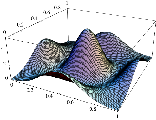
Figure 4. The function $\vartheta$ of Eq. (21) on $[0,1]^{2}$.

The functional relation (20) can now be employed to define an iterative calculation of $F$ as follows. One starts from $F^{(0)}(x,y)=xy$ (which corresponds to the measure $\,\mathrm{d}F^{(0)}=\lambda$) and continues with the iteration

(22) $$F^{(N+1)}(x,y)\,=\,\frac{1}{9}\int_{0}^{3x}\int_{0}^{3y}\vartheta\bigl{(}\frac{x}{3},\frac{y}{3}\bigr{)}\,\mathrm{d}F^{(N)}(x,y)\hskip 0.5pt.$$

The functions $F^{(N)}$ have the form

$$\begin{split}F^{(N)}(x,y)\,=&\;\,x\hskip 0.5pty+x\sum_{n=1}^{3^{N}-1}\frac{\beta^{(N)}_{0,n}}{\pi\hskip 0.5ptn}\sin(2\pi ny)+y\sum_{m=1}^{3^{N}-1}\frac{\beta^{(N)}_{m,0}}{\pi\hskip 0.5ptm}\sin(2\pi mx)\\ &\;+\sum_{m,n=1}^{3^{N}-1}\frac{\beta^{(N)}_{m,n}}{\pi^{2}\hskip 0.5ptmn}\sin(2\pi mx)\sin(2\pi ny)\hskip 0.5pt,\end{split}$$

where the coefficients $\beta^{(N)}_{m,n}$ are defined for $N,m,n\geq 0$ by the initial conditions $\beta^{(0)}_{m,n}=\delta_{m,0}\delta_{n,0}$ together with the recursion

$$\beta^{(N+1)}_{3m+r,3n+s}\,=\sum_{k=0}^{\min(1,r)}\sum_{\ell=0}^{\min(1,s)}\alpha^{(r,s)}_{k,\ell}\hskip 0.5pt\beta^{(N)}_{m+k,n+\ell}\hskip 0.5pt,$$

with $N\geq 0$ and the same coefficients $\alpha^{(r,s)}_{k,\ell}$ as in Eq. (9). This can once again be verified by a direct calculation.

All $F^{(N)}$ represent absolutely continuous measures, so that we can define Radon-Nikodym densities via $\,\mathrm{d}F^{(N)}(x,y)=f^{(N)}(x,y)\,\mathrm{d}x\,\mathrm{d}y$, where

$$f^{(N)}(x,y)\,=\,\frac{\partial^{2}}{\partial x\hskip 0.5pt\partial y}F^{(N)}(x,y)\hskip 0.5pt.$$

This gives $f^{(1)}=\vartheta$, with the function $\vartheta$ from Eq. (21), via the application of some trigonometric identities. The iteration now reveals the Riesz product formula

(23) $$f^{(N)}(x,y)\,=\prod_{\ell=0}^{N-1}\vartheta(3^{\ell}x,3^{\ell}y)\hskip 0.5pt,$$

which highlights the deeper role of $\vartheta$ in Eq. (22). The distribution function $F^{(3)}$ and the corresponding density $f^{(3)}$ are shown in Figure 5.

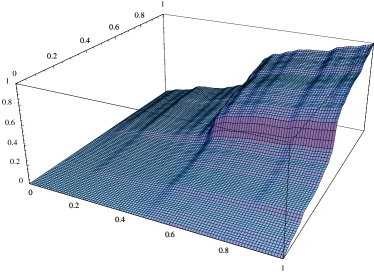
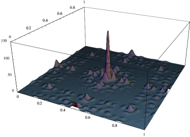
Figure 5. The distribution function $F^{(3)}$ of Eq. (22) (left) and the corresponding density $f^{(3)}$ of Eq. (23) (right), approximating the diffraction measure of the squiral tiling (in the version of Figure 2) on $[0,1]^{2}$.

Remark 3.

The measure defined by the continuous function $F$ is represented by the infinite Riesz product $\prod_{\ell=0}^{\infty}\vartheta(3^{\ell}x,3^{\ell}y)$, to be understood with convergence in the vague topology. By a comparison of Eqs. (20) and (22), it is clear that $F$ is a fixed point of the latter. In fact, within the class of distribution functions with certain continuity and additivity constraints, it is the only fixed point, with uniform (but not absolute) convergence towards it from the initial condition $F^{(0)}$, again by arguments analogous to [16, Thm. 30.13].

6. A topological factor with maximal pure point spectrum

It is well known that the one-dimensional Thue-Morse system admits a topological factor with maximal pure point spectrum, which can be defined by the period doubling substitution. In fact, the latter is induced by a simple sliding block map of width $2$. The corresponding factor map is globally $2$-to-$1$ between the hulls; see [6] for details and an extension to generalised Thue-Morse sequences. Amazingly, a similar approach also works for the squiral tiling.

Define the mapping $\psi\!:\,\{1,\bar{1}\}^{\mathbb{Z}^{2}}\longrightarrow\{1,\bar{1}\}^{\mathbb{Z}^{2}}$ by $w\mapsto\psi w$ with

$$(\psi w)_{m,n}\,=\,w_{m,n}w_{m+1,n}w_{m,n+1}w_{m+1,n+1}\hskip 0.5pt,$$

which is continuous. It is clear that $\mathbb{Y}:=\psi\mathbb{X}$ defines a factor for the action of $\mathbb{Z}^{2}$. Moreover, the inflation rule (1) induces a new inflation on $\mathbb{Y}$, which reads

(24) $$\begin{matrix}&&1&1&a\\ &&\bar{1}&\bar{1}&1\\ a&\longmapsto&\bar{1}&\bar{1}&1\end{matrix}$$

with $a\in\{1,\bar{1}\}$. Note that the arrangement matches that of the inflation rule (1). One checks consistency by starting from the $14$ legal patches with $2\times 2$ squares, and verifies that they inflate to larger patches that produce the correct $3\times 3$ blocks in the lower left corner under $\psi$. One can check that the block map is not globally $2$-to-$1$, though it is $2$-to-$1$ almost everywhere. For a more detailed discussion and a classification of the substitution factors of the squiral, we refer to [7].

Consider one of the two possible fixed points of the induced substitution (24) and decompose $\mathbb{Z}^{2}=\varLambda_{+}\operatorname{\dot{\cup}}\varLambda_{-}$, where $\varLambda_{\pm}=\{(m,n)\in\mathbb{Z}^{2}\mid w_{m,n}=\pm 1\}$. Using $e_{1}=(1,0)$ and $e_{2}=(0,1)$, the fixed point property now induces the set-valued relations

(25) $$\varLambda_{\pm}\,=\,\bigl{(}3\mathbb{Z}^{2}+S_{\pm}\bigr{)}\operatorname{\dot{\cup}}\,\bigl{(}3\varLambda_{\pm}+2(e_{1}\!+\!e_{2})\bigr{)}$$

with the translation sets $S_{+}=\{2e_{1},2e_{2},2e_{1}\!+\!e_{2},e_{1}\!+\!2e_{2}\}$ and $S_{-}=\{0,e_{1},e_{2},e_{1}\!+\!e_{2}\}$.

The solutions are

$$\varLambda_{\pm}\,=\,\operatorname*{\dot{\bigcup}}_{n\geq 1}\bigl{(}3^{n}\mathbb{Z}^{2}+3^{n-1}S_{\pm}+(3^{n-1}-1)(e_{1}\!+\!e_{2})\bigr{)}\;\operatorname{\dot{\cup}}\,A_{\pm}$$

where either $A_{+}=\{-(e_{1}\!+\!e_{2})\}$ and $A_{-}=\varnothing$, or vice versa. The special role of the point $(-1,-1)$ becomes transparent in the topology of the $3$-adic numbers.

The sets $\varLambda_{\pm}$ are model sets with two copies of the $3$-adic numbers as internal space. The Dirac combs $\delta_{\!\varLambda_{\pm}}$ are thus pure point diffractive by the model set theorem; see [43, Thm. 4.5] or [14, Thm. 2]. A standard calculation now reveals that the corresponding Fourier module is $\mathbb{Z}[\frac{1}{3}]\times\mathbb{Z}[\frac{1}{3}]$. By general arguments [33, 11], this equals the dynamical spectrum of $\mathbb{Y}$.

By the results of [20], the pure point part of the dynamical spectrum of $\mathbb{X}$ thus equals the dynamical spectrum of $\mathbb{Y}$, which shows that $\mathbb{Y}$ is indeed a topological factor that exhausts the pure point spectrum of the squiral tiling. To summarise, we have shown the following.

Theorem 2.

The squiral tiling dynamical system has a dynamical spectrum of mixed type, with pure point part $\mathbb{Z}[\frac{1}{3}]\times\mathbb{Z}[\frac{1}{3}]$ and an additional singular continuous part. The latter is exploited by the diffraction measure of the balanced Dirac comb of Eq. (3), while the former can be recovered from the pure point diffraction spectrum of the factor system defined via Eq. (24). ∎

7. Generalisations

When inspecting the structure of the above constructive approach, it is apparent that the method is not restricted to the particular example of the squiral tiling or its equivalent block substitution rule. Instead, one might as well consider a $d$-dimensional extension to bijective block substitutions on a binary alphabet as follows.

Let $K$ be a matrix array of dimension $K_{1}\times K_{2}\times\ldots\times K_{d}$, with all $K_{i}\geq 2$ and entries $\pm 1$ (with $\bar{1}=-1$ as before), not all equal. Now consider the rule

$$\varrho\!:\;1\longmapsto K\hskip 0.5pt,\;\bar{1}\longmapsto\bar{K}\hskip 0.5pt,$$

where $\bar{K}$ is obtained from $K$ by flipping all signs. This defines a primitive block substitution rule with substitution matrix $M=\left(\begin{smallmatrix}m&\bar{m}\\ \bar{m}&m\end{smallmatrix}\right)$, where $m$ is the cardinality of $1$s in $K$ and $\bar{m}$ that of $\bar{1}$s. The PF eigenvalue is $\prod_{i}K_{i}$, with (left and right) eigenvector given by $(1,1)$. This is in line with a tiling interpretation, with unit cubes of two colours as prototiles. They occur with equal frequency in any fixed point tiling.

Select any legal block patch of size $2\!\times\!2\!\times\!\ldots\!\times\!2$, which contains $2^{d}$ blocks, and take its centre as reference point (meaning that each sector of $\mathbb{Z}^{d}$ contains one block of it). This way, the origin is a corner of a block. Starting from such a seed, we can now iterate $\varrho$ to create a sequence of block patches that ultimately cover all positions of $\mathbb{Z}^{d}$, due to our assumption that all $K_{i}\geq 2$. Note that the block patches of type $K$ and $\bar{K}$ fit together in a face-to-face manner in this process.

Without loss of generality, we may now assume that we have constructed a fixed point in this way, which is possibly only true after replacing $\varrho$ by a suitable power of it, and modifying $K$ accordingly. This modification is always possible, as follows from an application of Dirichlet’s pigeon hole principle to the finite set of legal seeds. Note that any power of $\varrho$ still satisfies our basic assumptions, wherefore this step is immaterial for the arguments to follow (although it might technically complicate explicit calculations due to the increased size of the new array $K$).

Let $w$ be the fixed point under consideration. It is then specified by the recursion relations

(26) $$w_{K_{1}m_{1}+r_{1},\ldots,K_{d}m_{d}+r_{d}}\,=\,\hskip 0.5pt\kappa_{r_{1},\ldots,r_{d}}\hskip 0.5ptw_{m_{1},\ldots,m_{d}}$$

where all $m_{i}\in\mathbb{Z}$ and $0\leq r_{i}<K_{i}$, while the coefficients $\kappa_{r_{1},\ldots,r_{d}}\in\{\pm 1\}$ are the elements of $K$, numbered accordingly. Due to the primitivity of $\varrho$, the fixed point $w$ defines a repetitive configuration in the shift space $\{\pm 1\}^{\mathbb{Z}}$, wherefore it leads to a hull

$$\mathbb{X}\,=\,\mathbb{X}(w)\,:=\,\overline{\{t+w\mid t\in\mathbb{Z}^{d}\}}$$

that is a minimal subshift of $\{\pm 1\}^{\mathbb{Z}}$. Moreover, $(\mathbb{X},\mathbb{Z}^{d})$ defines a strictly ergodic dynamical system by standard arguments [41, 44, 20, 40].

If $\omega=w\hskip 0.5pt\delta_{\mathbb{Z}^{d}}$ is the attached Dirac comb, its autocorrelation $\gamma=\omega\circledast\widetilde{\omega}$ (defined in complete analogy to Eq. (4)) exists and is of the form $\gamma=\eta\hskip 0.5pt\delta_{\mathbb{Z}^{d}}$ with coefficients

(27) $$\eta\hskip 0.5pt(m_{1},\ldots,m_{d})\,=\lim_{N\to\infty}\frac{1}{(2N+1)^{d}}\sum_{k_{1}=-N}^{N}\dots\sum_{k_{d}=-N}^{N}w_{k_{1},\ldots,k_{d}}\,w_{k_{1}-m_{1},\ldots,k_{d}-m_{d}}\hskip 0.5pt.$$

The sums are orbit averages of a continuous function under the action of $\mathbb{Z}^{d}$, which always exist due to unique ergodicity (by an application of the stronger version of Birkhoff’s ergodic theorem [46]).

One can now repeat the constructive calculation of the squiral block substitution in this more general setting.

Lemma 6.

Let $\varrho$ be a primitive, bijective block substitution on a binary alphabet, with a fixed point configuration $w$ that satisfies Eq. (26). The corresponding autocorrelation coefficients satisfy $\eta\hskip 0.5pt(0,\ldots,0)=1$ together with the linear recursion relations

$$\eta\hskip 0.5pt(K_{1}m_{1}\!+\!\hskip 0.5ptr_{1},\ldots,K_{d}\hskip 0.5ptm_{d}\hskip 0.5pt\!+\!\hskip 0.5ptr_{d})\,=\sum_{s_{1}=0}^{1}\dots\sum_{s_{d}=0}^{1}\begin{pmatrix}r_{1},\ldots,r_{d}\\ s_{1},\ldots,s_{d}\end{pmatrix}\,\eta\hskip 0.5pt(m_{1}\!+\!\hskip 0.5pts_{1},\ldots,m_{d}\hskip 0.5pt\!+\!\hskip 0.5pts_{d})$$

with rational coefficients $\left(\begin{smallmatrix}r_{1},\ldots,r_{d}\\ s_{1},\ldots,s_{d}\end{smallmatrix}\right)$ of modulus $\leq 1$. This recursion determines all coefficients uniquely once the initial condition $\eta\hskip 0.5pt(0,\ldots,0)$ is given.

In particular, one has $\left(\begin{smallmatrix}0\,,\ldots,\hskip 0.5pt0\\ s_{1},\ldots,s_{d}\end{smallmatrix}\right)=\delta_{s_{1},0}\cdot\ldots\cdot\delta_{s_{d},0}$, so that the relation

$$\eta\hskip 0.5pt(K_{1}m_{1},\ldots,K_{d}\hskip 0.5ptm_{d})\,=\,\eta\hskip 0.5pt(m_{1},\ldots,m_{d})$$

holds for all $(m_{1},\ldots,m_{d})\in\mathbb{Z}^{d}$.

Proof.

It is clear that $\eta\hskip 0.5pt(0,\ldots,0)=1$. For a general $\eta\hskip 0.5pt(K_{1}m_{1}\!+\!\hskip 0.5ptr_{1},\ldots,K_{d}\hskip 0.5ptm_{d}\hskip 0.5pt\!+\!\hskip 0.5ptr_{d})$, we start from the right-hand side of Eq. (27) (for finite $N$) and split the summation over the $i$th index modulo $K_{i}$. For each term, we can now apply the recursion (26). The sum can then be regrouped to contribute to coefficients of the form $\eta\hskip 0.5pt(m_{1}\!+\!s_{1},\ldots,m_{d}\!+\!s_{d})$ with $0\leq s_{i}\leq 1$. In the limit as $N\to\infty$, the contributions sum up to

(28) $$\begin{pmatrix}r_{1},\ldots,r_{d}\\ s_{1},\ldots,s_{d}\end{pmatrix}\,=\,\sum_{t_{1}=s_{1}(K_{1}-r_{1})}^{K_{1}-1-r_{1}(1-s_{1})}\dots\sum_{t_{d}=s_{d}(K_{d}-r_{d})}^{K_{d}-1-r_{d}(1-s_{d})}\frac{\kappa_{t_{1},\ldots,t_{d}}\,\kappa_{t_{1}+r_{1}-s_{1}K_{1},\ldots,t_{d}+r_{d}-s_{d}K_{d}}}{K_{1}\cdot\ldots\cdot K_{d}}$$

which follows by carefully keeping track of the various overflow rules due to the calculations modulo $K_{i}$. The claim on the rationality and boundedness is then obvious.

Inspecting the equations for the autocorrelation coefficients, one notices that for some of them (for instance those with $m_{1}=\ldots=m_{d}=0$ and one $r_{i}=1$) the resulting equation is a linear equation for a single coefficient that occurs on both sides. The prefactor of this coefficient on the right hand side can never be $1$, as one can see from Eq. (28) together with the assumption that the $\kappa$-array does contain entries of both signs. So, this type of equation always has a unique solution in terms of $\eta\hskip 0.5pt(0,\ldots,0)$, which fixes this particular $\eta$ value. The same argument applies to all equations of this type. The remaining coefficients are then determined recursively, and the solution is unique as soon as $\eta\hskip 0.5pt(0,\ldots,0)$ is specified.

The final claim is clear for $s_{1}=\ldots=s_{d}=0$. If $s_{i}=1$ for some $i$, the corresponding sum is empty, and the coefficient vanishes. ∎

By construction, the mapping $\eta\!:\,\mathbb{Z}^{d}\longrightarrow\mathbb{R}\hskip 0.5pt$ is a positive definite function on $\mathbb{Z}^{d}$, with $\eta\hskip 0.5pt(0,\ldots,0)=1$. By the Herglotz-Bochner theorem, see [42] or Lemma 7 below, there is then a unique probability measure $\mu$ on $\mathbb{T}^{d}=[0,1)^{d}$ such that

(29) $$\eta\hskip 0.5pt(\boldsymbol{m})\,=\,\int_{0}^{1}\cdots\int_{0}^{1}\exp(2\pi\hskip 0.5pt\mathrm{i}\hskip 0.5pt\hskip 0.5pt\boldsymbol{mx})\,\mathrm{d}\mu(\boldsymbol{x})\hskip 0.5pt,$$

where we write $\boldsymbol{m}=(m_{1},\ldots,m_{d})$ etc. in the remainder of this section, with $\boldsymbol{mx}$ denoting the scalar product. The positive measure $\mu$ has a unique decomposition into three components,

$$\mu\,=\,\mu_{\mathsf{pp}}+\mu_{\mathsf{sc}}+\mu_{\mathsf{ac}}\hskip 0.5pt,$$

with Lebesgue measure (as the Haar measure on $\mathbb{T}^{d}$) as reference measure.

Proposition 2.

Let $\varrho$ be as in Lemma 6, with autocorrelation coefficients $\eta$ and associated positive measure $\mu$ on $\mathbb{T}^{d}$. Then, the spectral type of $\mu$ is pure, which means that it is either a pure point measure, a purely singular continuous measure, or a purely absolutely continuous measure.

Proof.

By standard arguments, we know that $\mu_{\mathsf{pp}}\perp\mu_{\mathsf{sc}}\perp\mu_{\mathsf{ac}}\perp\mu_{\mathsf{pp}}$ in the measure-theoretic sense. Now, the recursion relations imply a set of functional relations for $\mu$, which must hold for each component separately as a consequence of the orthogonality relations.

Defining $\eta_{\alpha}(\boldsymbol{m})=\check{\mu}_{\alpha}(\boldsymbol{m})$ for $\alpha\in\{\mathsf{pp},\mathsf{sc},\mathsf{ac}\}$ separately, each type of autocorrelation coefficient must then satisfy the same recursion relations as $\eta$ itself, subject to the condition

$$\eta\hskip 0.5pt(\boldsymbol{0})\,=\,\eta_{\mathsf{pp}}(\boldsymbol{0})+\eta_{\mathsf{sc}}(\boldsymbol{0})+\eta_{\mathsf{ac}}(\boldsymbol{0})\,=\,1\hskip 0.5pt.$$

Note that, due to the linearity of the recursion relations, this splitting indeed leads to a solution of the recursion with the correct initial condition, hence the unique solution stated in Lemma 6.

This observation means that the three components of $\eta\hskip 0.5pt(\boldsymbol{m})$ are proportional according to their individual initial conditions $\eta_{\alpha}(\boldsymbol{0})$, so cannot produce different spectral type. This is only compatible with the claim made, and the type is pure. ∎

Let us take a closer look at the spectral types. Assume that the measure $\mu$ is absolutely continuous. Then, the Riemann-Lebesgue Lemma tells us that $\eta\hskip 0.5pt(\boldsymbol{m})=\eta_{\mathsf{ac}}(\boldsymbol{m})\longrightarrow 0$ as $\lvert\boldsymbol{m}\rvert\to\infty$. Recalling the last claim of Lemma 6, it follows that we must have $\eta\hskip 0.5pt(\boldsymbol{m})=0$ for all $\boldsymbol{m}\neq\boldsymbol{0}$, and hence $\eta\hskip 0.5pt(\boldsymbol{m})=\delta_{\boldsymbol{m},\boldsymbol{0}}$. This would imply $\mu$ to be Lebesgue measure on $\mathbb{T}^{d}$. A careful inspection of the recursion reveals that this outcome is only possible if all coefficients of type $\left(\begin{smallmatrix}r_{1},\ldots,r_{d}\\ 0\,,\ldots,\,0\end{smallmatrix}\right)$ vanish. However, we have

$$\left(\begin{array}[]{@{}c@{}c@{}c@{}}K_{1}\!-\!1&,\ldots,&K_{d}\!-\!1\\ 0&,\ldots,&0\end{array}\right)\,=\,\frac{\kappa_{0,\ldots,0}\,\kappa_{K_{1}-1,\ldots,K_{d}-1}}{K_{1}\cdot\ldots\cdot K_{d}}\,\neq\,0$$

which excludes this possibility. Consequently, the measure $\mu$ in Proposition 2 is a singular measure.

Put together, we have proved the following result.

Theorem 3.

Let $\varrho$ be a primitive, bijective block substitution on $\mathbb{Z}^{d}$, for a binary alphabet. Assume that it is extensive in all directions, and let $w$ be a fixed point configuration that satisfies Eq. (26) on $\mathbb{Z}^{d}$.

If $\eta$ is the corresponding autocorrelation function on $\mathbb{Z}^{d}$, and $\mu$ the attached positive measure on $\mathbb{T}^{d}$ according to Eq. (29), the measure $\mu$ is singular. In particular, it is either pure point or purely singular continuous. ∎

Both possibilities clearly occur. Examples for pure point cases can be constructed via substitutions that have fully periodic fixed points. Such fixed points usually have non-trivial height lattices, and are thus of limited interest; see [20, Sec. 3.1] for the precise definition of the height lattice of a $\mathbb{Z}^{d}$ lattice substitution. If the height lattice of a primitive bijective substitution is trivial, one can construct a cyclic space in the complement of the span of the eigenfunctions [20, 21]. Its spectral measure is nothing but our measure $\mu$, which is then inevitably singular continuous.

Corollary 1.

If the block substitution from Theorem 3 has trivial height, the diffraction measure of the corresponding balanced Dirac comb is purely singular continuous. ∎

Remark 4.

Singular continuity of a (positive) measure $\mu$ comprises rather different situations in $d>1$ dimensions. For instance, $\mu$ can be genuinely singular continuous, such as the measure of our squiral tiling above. However, one can also find product measures of a different kind. As an example, consider the primitive, bijective block substitution defined by

$$\begin{array}[]{ccccc}&&\bar{1}&1&\bar{1}\\ 1&\longmapsto&1&\bar{1}&1\end{array}$$

in symbolic notation on the binary alphabet $\{1,\bar{1}\}$. This rule defines a hull that is $2$-periodic in the horizontal direction and Thue-Morse in the vertical one. Consequently, the measure $\mu$ in this case is a product measure, written as $\mu=\mu_{1}\otimes\mu_{2}$, where $\mu_{1}$ is a pure point measure and $\mu_{2}$ is the classic TM measure. Nevertheless, $\mu$ is purely singular continuous as a measure on $\mathbb{T}^{2}$. This is an example with a non-trivial height lattice that still shows purely singular continuous diffraction, though the corresponding distribution function is not continuous.

Let us assume that the probability measure $\mu$ from Eq. (29) is purely singular continuous and that the distribution function $F$ for $\widehat{\gamma}=\mu*\delta_{\mathbb{Z}^{d}}$ is continuous (which excludes examples such as those mentioned in Remark 4). The latter condition is equivalent to the $d$ one-dimensional distribution functions $F(1,\ldots,1,x_{i},1,\ldots,1)$ being continuous, by an application of [45, Thm. 2.3]. Then, the recursion relation for the autocorrelation coefficients $\eta$ can meaningfully be turned into an iteration, as in our planar example. One can then derive an explicit representation of $\mu$ (and hence also $\widehat{\gamma}$) as a (generalised) Riesz product in this case. In particular, iterating the corresponding functional equation once with initial condition $F^{(0)}(\boldsymbol{x})=\prod_{i=1}^{d}x_{i}$ leads to $F^{(1)}$, with density function

$$f^{(1)}(\boldsymbol{x})\,=\,\frac{\partial^{d}}{\partial x_{1}\dots\partial x_{d}}F^{(1)}(\boldsymbol{x})\hskip 0.5pt,$$

which plays the role of the trigonometric function $\vartheta$ in this more general setting. It can directly be calculated by means of the recursion coefficients as

(30) $$\vartheta(\boldsymbol{x})\,=\sum_{r_{1}=1-K_{1}}^{K_{1}-1}\dots\sum_{r_{d}=1-K_{d}}^{K_{d}-1}\begin{pmatrix}\lvert r_{1}\rvert,\ldots,\lvert r_{d}\rvert\\ 0\;\,,\ldots,\;\,0\end{pmatrix}\prod_{i=1}^{d}\cos(2\pi r_{i}\hskip 0.5ptx_{i})\hskip 0.5pt,$$

which defines a non-negative function on $\mathbb{R}\hskip 0.5pt^{d}$ with $\int_{\mathbb{T}^{d}}\vartheta(\boldsymbol{x})\,\mathrm{d}\boldsymbol{x}=1$. This leads to $f^{(N)}(\boldsymbol{x})=\prod_{\ell=0}^{N-1}\vartheta(K_{1}^{\ell}x_{1},\ldots,K_{d}^{\ell}x_{d})$ and thus to an infinite Riesz product for the diffraction measure $\widehat{\gamma}$. The distribution function can also be written as

$$F(\boldsymbol{x})\,=\,x_{1}\cdot\ldots\cdot x_{d}\sum_{\boldsymbol{m}\in\mathbb{Z}^{d}}\eta\hskip 0.5pt(\boldsymbol{m})\prod_{i=1}^{d}\mathrm{sinc}(2\pi m_{i}x_{i})\hskip 0.5pt,$$

in complete analogy to our previous formulas of this type.

A complete classification of the cases with pure point spectrum and an extension to larger alphabets remain as interesting open problems. Another question concerns a better understanding of the topological factors of bijective substitutions. We expect a complete correspondence between the original dynamical spectrum and the diffraction spectra of the system and its factors.

Appendix

Let us formulate Wiener’s lemma for the group $\mathbb{Z}^{d}$, which is a straight-forward generalisation of the case $d=1$ in [37, Sec. 4.16]. Here, $C_{n}=\{u\in\mathbb{R}\hskip 0.5pt^{d}\mid\|u\|_{\infty}\leq n\}$ denotes the closed cube of sidelength $2n$, centred at the origin. One has $\mathrm{card}(\mathbb{Z}^{d}\cap C_{n})=(2n\!+\!1)^{d}$.

Lemma 7.

If $\eta\!:\,\mathbb{Z}^{d}\longrightarrow\mathbb{C}\hskip 0.5pt$ is positive definite, there is a unique positive measure $\mu$ on $\mathbb{T}^{d}\simeq\mathbb{R}\hskip 0.5pt^{d}/\mathbb{Z}^{d}$ such that

$$\eta\hskip 0.5pt(k)\,=\int_{\mathbb{T}^{d}}\,\mathrm{e}^{2\pi\hskip 0.5pt\mathrm{i}ku}\,\mathrm{d}\mu(u)$$

holds for all $k\in\mathbb{Z}^{d}$. When $\eta\hskip 0.5pt(0)=1$, the measure $\mu$ is a probability measure on $\mathbb{T}^{d}$.

Moreover, one has the relation

$$\lim_{n\to\infty}\frac{1}{(2n+1)^{d}}\sum_{k\in\mathbb{Z}^{d}\cap C_{n}}\bigl{|}\eta\hskip 0.5pt(k)\bigr{|}^{2}\,=\,\sum_{t\in\mathbb{T}^{d}}\bigl{(}\mu(\{t\})\bigr{)}^{2},$$

where the last sum runs over at most countably many points.

Proof.

Since $\mathbb{Z}^{d}$ and $\mathbb{T}^{d}$ form a mutually dual pair of locally compact Abelian groups, the first claim is just the Herglotz-Bochner theorem for this situation, compare [42], with $\mu(\mathbb{T}^{d})=\eta\hskip 0.5pt(0)$.

Now, define $g_{n}(u)=\frac{1}{(2n+1)^{d}}\sum_{k\in\mathbb{Z}^{d}\cap C_{n}}\,\mathrm{e}^{2\pi\hskip 0.5pt\mathrm{i}ku}$, which is bounded by $1$. It is not difficult to see that $g_{n}(u)\xrightarrow{\,n\to\infty\,}1_{\{0\}}(u)$ holds for any $u\in\mathbb{T}^{d}=[0,1)^{d}$. Using Fubini’s theorem and noting that $\bar{\mu}=\mu$, one obtains

$$\begin{split}\frac{1}{(2n\!+\!1)^{d}}&\sum_{k\in\mathbb{Z}^{d}\cap C_{n}}\!\!\bigl{|}\eta\hskip 0.5pt(k)\bigr{|}^{2}\,=\,\frac{1}{(2n\!+\!1)^{d}}\sum_{k\in\mathbb{Z}^{d}\cap C_{n}}\int_{\mathbb{T}^{d}}\!\,\mathrm{e}^{2\pi\hskip 0.5pt\mathrm{i}ku}\,\mathrm{d}\mu(u)\overline{\int_{\mathbb{T}^{d}}\!\,\mathrm{e}^{2\pi\hskip 0.5pt\mathrm{i}kv}\,\mathrm{d}\mu(v)}\\ &=\int_{\mathbb{T}^{d}\times\mathbb{T}^{d}}g_{n}(u-v)\,\mathrm{d}\mu(u)\,\mathrm{d}\mu(v)\;\,\xrightarrow{\,n\to\infty\,}\,\int_{\mathbb{T}^{d}\times\mathbb{T}^{d}}1_{\{0\}}(u-v)\,\mathrm{d}\mu(u)\,\mathrm{d}\mu(v)\end{split}$$

where the last step follows from dominated convergence; compare [38, Thm. 6.1.15] for a formulation in sufficient generality. The integral over the diagonal evaluates via Fubini’s theorem as

$$\int_{\mathbb{T}^{d}}\int_{\mathbb{T}^{d}}1_{\{0\}}(u-v)\,\mathrm{d}\mu(u)\,\mathrm{d}\mu(v)\,=\int_{\mathbb{T}^{d}}\mu(\{v\})\,\mathrm{d}\mu(v)\,=\sum_{t\in\mathbb{T}^{d}}\bigl{(}\mu(\{t\})\bigr{)}^{2},$$

where the last sum (since $\mu$ is a positive measure) runs over all points $t\in\mathbb{T}^{d}$ with $\mu(\{t\})>0$, which are (at most) countably many. ∎

References

- [1] Alimov Sh A, Ashurov R R and Pulatov A K, Multiple Fourier series and Fourier integrals, in: Commutative Harmonic Analysis IV, eds V P Khavin and N K Nikol’skiĭ, Springer, Berlin (1992) pp. 1–96.
- [2] Allouche J-P and Shallit J, Automatic Sequences: Theory, Applications, Generalizations, Cambridge University Press, Cambridge (2003).
- [3] Baake M, A guide to mathematical quasicrystals, in: Quasicrystals – An Introduction to Structure, Physical Properties and Applications, eds J-B Suck, M Schreiber and P Häussler, Springer, Berlin (2002) pp. 17–48; arXiv:math-ph/9901014.
-
[4]
Baake M,
Diffraction of weighted lattice subsets,
Can. Math. Bulletin 45 (2002) 483–498;
arXiv:math.MG/0106111. - [5] Baake M, Birkner M and Moody R V, Diffraction of stochastic point sets: Explicitly computable examples, Commun. Math. Phys. 293 (2010) 611–660; arXiv:0803.1266.
- [6] Baake M, Gähler F and Grimm U, Spectral and topological properties of a family of generalised Thue-Morse sequences, J. Math. Phys. 53 (2012) 032701; arXiv:1201.1423.
- [7] Baake M, Gähler F and Grimm U, The squiral tiling and its topological substitution factors, in preparation.
- [8] Baake M and Grimm U, The singular continuous diffraction measure of the Thue-Morse chain, J. Phys. A: Math. Theor. 41 (2008) 422001; arXiv:0809.0580.
-
[9]
Baake M and Grimm U,
Surprises in aperiodic diffraction,
J. Physics: Conf. Ser. 226 (2010) 012023;
arXiv:0909.5605. - [10] Baake M and Grimm U, Kinematic diffraction from a mathematical viewpoint, Z. Krist. 226 (2011) 711–725; arXiv:1105.0095.
- [11] Baake M and Lenz D, Dynamical systems on translation bounded measures: Pure point dynamical and diffraction spectra, Ergodic Th. & Dynam. Syst. 24 (2004) 1867–1893; math.DS/0302231.
- [12] Baake M, Lenz D and Moody R V, Characterization of model sets by dynamical systems, Ergodic Th. & Dynam. Syst. 27 (2007) 341–382; arXiv:math.DS/0511648.
- [13] Baake M and Moody R V (eds.), Directions in Mathematical Quasicrystals, CRM Monograph Series vol. 13, AMS. Providence, RI (2000)
- [14] Baake M and Moody R V, Weighted Dirac combs with pure point diffraction, J. reine angew. Math. (Crelle) 573 (2004) 61–94; arXiv:math/0203030.
- [15] Baake M, Schlottmann M and Jarvis P D, Quasiperiodic patterns with tenfold symmetry and equivalence with respect to local derivability, J. Phys. A: Math. Gen. 24 (1991) 4637–4654.
- [16] Bauer H, Measure and Integration Theory, de Gruyter, Berlin (2001).
- [17] Billingsley P, Probability and Measure, 3rd ed., Wiley, New York (1995).
- [18] Cowley J M, Diffraction Physics, 3rd ed., North-Holland, Amsterdam (1995).
- [19] Dekking F M, The spectrum of dynamical systems arising from substitutions of constant length, Z. Wahrscheinlichkeitsth. verw. Geb. 41 (1978) 221–239.
- [20] Frank N P, Multi-dimensional constant-length substitution sequences, Topol. Appl. 152 (2005) 44–69.
- [21] Frank N P, Spectral theory of bijective substitution sequences, MFO Reports 6 (2009) 752–756.
- [22] Frettlöh D, Nichtperiodische Pflasterungen mit ganzzahligem Inflationsfaktor, PhD thesis, Univ. Dortmund (2002).
- [23] Frettlöh D and Sing B, Computing modular coincidences for substitution tilings and point sets, Discr. Comput. Geom. 37 (2007) 381–407; arXiv:math.MG/0601067.
- [24] Gnedenko B V, The Theory of Probability and The Elements of Statistics, 4th ed., reprint, AMS Chelsea, Providence (2005).
- [25] Grünbaum B and Shephard G C, Tilings and Patterns, Freeman, New York (1987).
-
[26]
Höffe M and Baake M,
Surprises in diffuse scattering,
Z. Krist. 215 (2000) 441–444;
arXiv:math-ph/0004022. - [27] Hof A, On diffraction by aperiodic structures, Commun. Math. Phys. 169 (1995) 25–43.
- [28] Kakutani S, Strictly ergodic symbolic dynamical systems, Proc. 6th Berkeley Symposium on Math. Statistics and Probability eds L M LeCam, J Neyman and E L Scott, Univ. of California Press, Berkeley (1972), pp. 319–326.
- [29] Katznelson Y, An Introduction to Harmonic Analysis, 3rd ed., Cambridge University Press, New York (2004).
- [30] Keane M, Generalized Morse sequences, Z. Wahrscheinlichkeitsth. verw. Geb. 10 (1968) 335–353.
- [31] Lagarias J C and Pleasants P A B, Repetitive Delone sets and quasicrystals, Ergod. Th. & Dynam. Syst. 23 (2003) 831–867; arXiv:math.DS/9909033.
- [32] Lee J-Y and Moody R V, Lattice substitution systems and model sets, Discr. Comput. Geom. 25 (2001) 173–201; arXiv:math.MG/0002019.
- [33] Lee J-Y, Moody R V, and Solomyak B, Pure point dynamical and diffraction spectra, Ann. H. Poincaré 3, 1003–1018; arXiv:0910.4809.
- [34] Lee J-Y, Moody R V, and Solomyak B, Consequences of pure point diffraction spectra for multiset substitution systems, Discr. Comput. Geom. 29 (2003) 525–560; arXiv:0910.4450.
- [35] Lenz D and Moody R V, Stationary processes with pure point diffraction, preprint arXiv:1111.3617.
- [36] Mahler K, The spectrum of an array and its application to the study of the translation properties of a simple class of arithmetical functions. Part II: On the translation properties of a simple class of arithmetical functions, J. Math. Massachusetts 6 (1927) 158–163.
- [37] Nadkarni M G, Basic Ergodic Theory, 2nd ed., Birkhäuser, Basel (1995).
- [38] Pedersen G K, Analysis Now, rev. printing, Springer, New York (1995).
- [39] Pinsky M A, Introduction to Fourier Analysis and Wavelets, Brooks/Cole, Pacific Grove, CA (2002).
- [40] Queffélec M, Substitution Dynamical Systems – Spectral Analysis, LNM 1294, 2nd ed., Springer, Berlin (2010).
- [41] Robinson E A, Symbolic dynamics and tilings of , Proc. Sympos. Appl. Math. 60 (2004) 81–119.
- [42] Rudin W, Fourier Analysis on Groups, reprint, Wiley, New York (1990).
- [43] Schlottmann M, Generalised model sets and dynamical systems, in: [13], pp. 143–159.
- [44] Solomyak B, Dynamics of self-similar tilings, Ergod. Th. & Dynam. Syst. 17 (1997) 695–738 and 19 (1999) 1685 (Erratum).
- [45] Tucker H G, A Graduate Course in Probability, Academic Press, New York (1967).
- [46] Walters P, An Introduction to Ergodic Theory, reprint, Springer, New York (2000).
- [47] Wiener N, The spectrum of an array and its application to the study of the translation properties of a simple class of arithmetical functions. Part I: The spectrum of an array, J. Math. Massachusetts 6 (1927) 145–157.
- [48] Withers R L, Disorder, structured diffuse scattering and the transmission electron microscope, Z. Krist. 220 (2005) 1027–1034.
- [49] Zaks M A, On the dimensions of the spectral measure of symmetric binary substitutions, J. Phys. A: Math. Gen. 35 (2002) 5833–5841.
- [50] Zygmund A, Trigonometric Series, 3rd ed., Cambridge University Press, Cambridge (2002).