Direct modeling of neutral helium in the heliosphere

Abstract

Several years of neutral particle measurements by the NASA/IBEX mission have yielded direct observations of interstellar neutral helium and oxygen. The data indicate the presence of secondary neutral helium and oxygen, which are created within the heliosphere by charge exchange involving helium or oxygen ions. This contribution describes a detailed conserving calculation method based on Keplerian orbits that has been developed to characterize helium distribution functions throughout the heliosphere, in particular in the innermost heliosphere, while accounting for loss and production of neutral particles along their path. Coupled with global heliosphere models of plasma distributions, this code is useful for predicting the fluxes of heavy neutral atoms at spacecraft detectors, so enabling inferences on the characteristics of the interstellar medium.

1 Introduction

On its galactic journey, the Sun traverses a cloud of interstellar gas that is moderately warm and dense, and is partially ionized, meaning that it also contains neutral atoms (dominantly hydrogen, but also helium, oxygen, and others). While the interstellar plasma interacts with the solar wind to form the global heliosphere, interstellar neutrals are unaffected and proceed into the heliosphere in their original velocity state. As such they are direct messengers of the interstellar medium, detectable by spacecraft in the inner solar system (like NASA/IBEX; Bzowski et al. 2012; Möbius et al. 2012). This has intensified interest in accurate heliospheric neutral modeling, including secondaries.

The entrance of heavy interstellar neutrals into the heliosphere has been modeled in detail in the past (e.g., Müller & Zank 2004; Izmodenov et al. 2004; Bzowski et al. 2012, and references therein). These calculations are typically variants of models and calculations of neutral interstellar hydrogen in the heliosphere, which have a long history spanning four decades (for reviews, see Axford 1972; Zank 1999; Izmodenov 2006). Simulations treat the heavies as test particles on the background of the global hydrogen/proton heliosphere. Monte-Carlo methods are useful in the global heliosphere, but statistics are poorer in the innermost heliosphere where IBEX measures. Reverse-trajectory methods are therefore popular to calculate heavy neutrals in the heliosphere, but typically the input flux is approximated at an outer boundary that is still well inside the heliosphere. This paper focuses on a method combining the best of both approaches, starting from the pristine interstellar medium, but calculating the phase space distribution function (PDF) at an arbitrary point of interest in a conserved way through reverse trajectories while allowing for arbitrary ionization (loss) and production terms.

2 Scientific framework and numerical details

In a heliocentric frame of reference, the motion of the neutrals is governed by the central gravitational potential of the Sun, such that the neutrals are on Keplerian trajectories, their paths deflected close to the Sun. The potential is weak for hydrogen which experiences an additional outward radiation pressure force that balances most of gravity. During solar maximum when radiation levels are highest in the solar cycle, radiation even overcompensates gravity, leading to an effectively repulsive potential for hydrogen during these times. Heavy neutrals are easier to handle, and the unimportance of radiation pressure for them means that the corresponding central potential is conservative and time-independent.

Primary (interstellar) particles are on open trajectories (hyperbolae, and possibly parabolae as limiting case). Each individual trajectory can be described geometrically by specifying the orbital plane, the direction of perihelion, and the orbital eccentricity $e$. If $\theta$, the angle that a particle’s position vector makes with the direction of perihelion, is given, then the particle’s radial distance and velocity are determined with simple formulae from celestial mechanics ($r(\theta)$; $v_{r}(\theta)$; $v_{\theta}(\theta)$); the time to or since perihelion $t(\theta)$ can also be obtained relatively easy albeit not in closed form. If any of the latter quantities is given instead, the other variables are determined just as easy from it, even if sometimes two solutions arise describing situations which are symmetric with respect to the perihelion (e.g., $\theta(r)$). Each individual trajectory can also alternatively be described physically by specifying conserved quantities including total specific energy $E$, specific angular momentum $\vec{l}$, and the eccentricity vector $\vec{a}$ (Müller & Cohen 2012). Again with trajectories defined in this manner, any one given value for angle, distance, velocity or time will yield all the respective others. There are of course numerous relations that link orbital elements to the physical quantities (for instance, the orbital plane is perpendicular to $\vec{l}$, and $e$ and the perihelion distance $r_{min}$ depend only on $l$ and $E$).

On their way through the heliosphere, atoms have a probability of being lost. In the case of interstellar helium, in order of importance for helium atoms detected at a 1 AU distance (e.g., location of IBEX), the processes are loss due to photoionization, loss due to charge exchange (c.x.) with slow helium ions in the outer heliosheath, double-c.x. with solar wind alpha particles, and c.x. with solar wind protons (Bzowski et al. 2012). Earlier studies (e.g., Müller & Zank 2004) were limited in admitting only c.x. with protons as a loss process. Secondary helium is created as the neutral product of a c.x. collision between a helium ion and a neutral, the dominant interaction being bow-shock decelerated interstellar He⁺ exchanging charge with interstellar helium in the outer heliosheath (loss of a primary particle and at the same time creation of a secondary neutral in a different velocity state, reflecting the underlying plasma distribution function). Of course, once created, a secondary neutral on its further trajectory suffers the same types of losses as the primary neutrals.

Two frames of reference are most appropriate for the neutral calculations: (1) The “ISM frame” in which the $x$ axis points antiparallel to the interstellar (ISM) flow so that the ISM flow vector at infinity is $(u_{x,ISM},0,0)$ with $u_{x,ISM}=-26.3$ km/s (Witte 2004); and (2) the “Kepler frame” in which the $x$ axis points to the perihelion of the trajectory in question, and the $x$-$y$ plane is the orbital plane. For each trajectory, $a_{z}=l_{x}=l_{y}=0$ in its Kepler frame, leading to a convenient reduction of conserved quantities that need to be considered. Rotation transformations relate ISM frame coordinates to Kepler frame coordinates, and also to other coordinates of choice such as a heliocentric frame of reference associated with ecliptic longitude and latitude. Spherical polar coordinates like the latter are typically used for the heliosphere plasma background model. $r$ is invariant under these transformations.

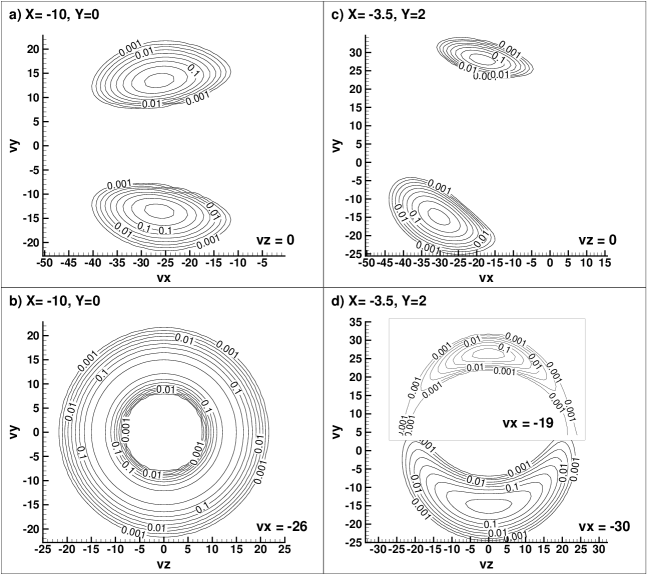
Figure 1.: Phase space densities of primary neutral interstellar helium at downwind locations, on the symmetry axis ((-10.0, 0.0), panels (a) and (b)), and at a location slightly off the symmetry axis at (-3.5, 2.0), distance 4.0 AU (panels (c) and (d)). Both locations are in the helium focusing cone, with the PSD being a deformed torus loosely perpendicular to the $x$-axis; see text for details. Presented for each PSD are two perpendicular cuts through the 3D object, with the cut plane specified (panel (d) and its inset have different cut planes, as indicated). The maximum PSD value in the ISM is normalized to 1 (logarithmic contour levels with 3 lines per dex.

The strategy to calculate a phase space distribution function (PDF) at a point of interest $\vec{r}_{0}$ is essentially to investigate all possible trajectories that pass through $\vec{r}_{0}$. For the primary PDF some of these trajectories have to be disregarded because they are not connected to the ISM (everything outside of the heliospheric bow shock); similarly, some trajectories that do not intersect with the outer heliosheath do not contribute towards the secondary PDF. In principle, all these trajectories passing through $\vec{r}_{0}$ can be obtained by scanning the entire 3D velocity space; for each individual phase space location $(\vec{r}_{0},\vec{v}_{0})$, the reverse trajectory is uniquely determined and the velocity at infinity, or at any point where the trajectory intersects the outer heliosheath, is calculated in one algebraic step, while preserving the conserved quantities by design.

Neglecting secondary neutrals for the moment, the prescription for the primary PDF is then as follows: By Liouville’s theorem, the raw phase space density at $(\vec{r}_{0},\vec{v}_{0})$ is the same as the value of the ISM Maxwellian at the calculated velocity at infinity. Attenuation factors arise due to photoionization and charge exchange; the photoionization factor can be cast into an analytic form involving essentially only expressions for $\theta$ and for the asymptotic $\theta_{\infty}$ at infinity, the latter a function of $e$. As we want to take the plasma background from an external global heliosphere model, the c.x. attenuation requires a c.x. loss integration along the trajectory from infinity (in reality, from the bow shock crossing) to $\vec{r}_{0}$, which is carried out at the $r$-grid nodes of the background model, with $\theta(r)$ determined algebraically (conserving by design) and the transformation matrix between Kepler and global heliosphere frames being constant during this calculation.

In practice, instead of 3D scanning, the locations of local maxima in the PDF are predicted algebraically: There are typically two maxima associated with the primary neutrals, called direct- and indirect-path velocities, where the indirect path is longer and leads the particle closer to the Sun (e.g., Müller & Cohen 2012). These velocities can be obtained in one step in the ISM frame by requiring the velocity at infinity to be $u_{x,ISM}$, which is the location of the maximum of the ISM Maxwellian:

$$(v_{x},v_{y})=(u_{x,ISM},0)-{f_{\mu}\over r_{0}l_{z}}(y,r_{0}-x)\,;\,\,\,l_{z}=-\frac{y\,u_{x,ISM}}{2}\left(1\pm\sqrt{1+4{f_{\mu}\over u_{x,ISM}^{2}}{r_{0}-x\over y^{2}}}\right)$$ (1)

with $(x,y)\equiv\vec{r}_{0}$, $f_{\mu}$ the constant of gravity multiplied by the solar mass, and the upper sign the direct path. The derivation typically makes use of the conserved quantities; similar results have been summarized by Axford (1972) and others.

The simplest practical strategy for the primary helium PDF is hence to obtain the location of the two maxima with equation (1), and then scan velocity space around them until the phase space density has dropped off by, say, 4 orders of magnitude which is equivalent to $\sim$4 thermal velocities, beyond which it can safely be neglected. A more sophisticated procedure is to develop the equivalent of eq. (1) for the fixed ISM frame with arbitrary interstellar vectors $\vec{u}$ and with it, map the locus of the edge of the ISM Maxwellian to velocities at $\vec{r}_{0}$. This gives a closed velocity surface at $\vec{r}_{0}$ within which the non-negligible PDF resides.

3 Primary helium results

Figure 1 shows two examples of applying the code, using typical ISM characteristics (Witte 2004), a typical heliospheric background model (Müller et al. 2006), and typical photoionization and c.x. rates. In the helium focusing cone on the downwind symmetry axis (Fig. 1a, b), the primary helium PSD is degenerate, with all planes containing the symmetry axis being equally preferred orbital planes for the interstellar particles. This leads to a torus-like PDF, with the torus perpendicular to the $v_{x}$ axis and the cross section of the torus slightly gravitationally deformed away from a circular shape. The locus of maxima (64% of the interstellar Maxwellian maximum due to losses) is a circle with radius $\sqrt{-2f_{\mu}/x}=13.3$ km/s at a constant $v_{x}=u_{x,ISM}$.

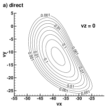
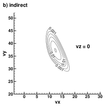
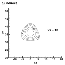
Figure 2.: Phase space density cuts of primary neutral interstellar helium at a sidewind location (0, 2) through the direct (a) and the indirect (b, c) PDF.

Moving $\vec{r}_{0}$ slightly off the symmetry axis (Fig. 1c, d), it can be seen that the degeneracy is broken. The plane of the torus is now tilted with respect to the $v_{y}$-$v_{z}$ plane, and the torus now connects a thick knot (maximum 62%) to a small knot (34%), with the connections having only very low phase space density. Going further off-axis makes it clear that the thick knot is associated with direct path trajectories; the small knot is associated with the indirect path (more prone to losses and hence less dense), and they are no longer connected. Inspecting upwind directions, the direct portion approaches a Maxwellian, whereas the indirect portion is severely deformed, having to travel to the Sun first and then back to the point of interest, with the incumbent losses along the way.

An intermediate situation is shown in Figure 2, for the sidewind location (0, 2). Direct and indirect PDF are well separated. The direct peak (64%) occurs for negative $v_{x}$ and negative $v_{y}$, whereas both are positive for the indirect peak (5%). The 3D shapes are lenticular for the direct PDF, and even more irregular for the indirect one. The velocity volume occupied by these PDF traces back to the ISM and its Maxwellian. In configuration space, all the associated trajectories go through the location (0, 2), but at a remote reference distance, for example a sphere of radius 1000 AU, they fill a certain area. Note that not all interstellar particles passing through that area intersect the location (0, 2); in that sense, one can only talk about mapping the ISM Maxwellian to the PDF at (0, 2) in velocity space, but not in configuration space.

With the fast, accurate characterization of the neutral PDF in hand, it is straightforward to perform integrals in velocity space including moments of the PDF, to arrive at configuration space maps of number density, bulk velocity, temperature, loss and production rate, and others. All of these quantities also can be obtained separately for direct and indirect neutrals. Given the secondary production rate, through forward calculation the peak of the secondary PDF at an arbitrary location $\vec{r}_{0}$ can be constrained, making the calculation of the secondary PDF (scanning a velocity neighborhood of the expected center) more efficient. As mentioned above, for each individual secondary PDF point, an integration (nominally from bow shock to heliopause) is necessary to sum up the production terms and convolve the integration as usual with losses on the way to $\vec{r}_{0}$. This integration involves the knowledge of the primary PDF, and as such, the process has a recursive flavor to it. As seen from the vantage of heliospheric physics, one of the less resolved ingredients in the problem of secondary PDF is how the helium ions necessary for c.x. are being handled correctly. This problem is outside the purview of the neutral solver exhibited in this contribution, but pertains more to the correct handling of heavy ions through the global plasma heliosphere models.

4 Conclusions

Using the Kepler equations of celestial mechanics is an elegant, fast way to calculate trajectories of neutral heavy atoms originating in the local interstellar medium. The associated conserved quantities enable one-step calculations of particle locations and velocities that are accurate by design. The presented examples for helium show the sometimes complicated heliospheric phase space distribution functions. They emphasize the role of gravitational deflection and the effect of loss and production processes on the helium phase space distribution. The primary neutral helium PDF can be calculated in this way at any arbitrary point in the heliosphere, and its various moments yield maps of effective temperature, bulk velocity, and density. The latter are elevated in the region of the helium focusing cone, which is also where direct and indirect solutions merge together and therefore become equally important.

The developed computational method, if applied only to primaries, is somewhat parallel to the hot model of neutrals (Fahr 1971). Yet the same method applies to secondary helium neutrals as well, which is a novel feature. The method furthermore treats the plasma as background and therefore can be used with a variety of global heliospheric models to study the sensitivity of the helium signal to heliospheric asymmetries or other differences in the global models. Lastly, the mathematics of the method are not affected by a time-dependence neither of the background plasma nor of the photoionization rate; the method is therefore adaptable to realistic, time-dependent scenarios, necessitating only an increased level of housekeeping to match times in the trajectory with the time-dependent inputs.

Acknowledgments

Partial support of this work by NASA grants NNX10AC44G, NNX11AB48G, NNX10AE46G, and by a University of Chicago subcontract of NASA grant NNG05EC85C is gratefully acknowledged. The author thanks Vladimir Florinski, Priscilla Frisch, and Gary Zank for helpful interactions.

References

- Axford (1972) Axford, W. I. 1972, in Solar Wind, edited by C. P. Sonett, P. J. Coleman, & J. M. Wilcox (NASA SP-308), 609
- Bzowski et al. (2012) Bzowski, M., Kubiak, M. A., Möbius, E., Bochsler, P., Leonhard, T., Heirtzler, D., Kucharek, H., Sokol, J. M., Hlond, M., Crew, G. B., Schwadron, N. A., Fuselier, S. A., & McComas, D. J. 2012, ApJS, 198, 12
- Fahr (1971) Fahr, H. J. 1971, A&A, 14, 263
- Izmodenov (2006) Izmodenov, V. V. 2006, in The Physics of the Heliospheric Boundaries, edited by V. V. Izmodenov, & R. Kallenbach (ISSI Sci. Rep. SR-005), 45
- Izmodenov et al. (2004) Izmodenov, V. V., Malama, Y. G., Gloeckler, G., & Geiss, J. 2004, A&A, 414, L29
- Möbius et al. (2012) Möbius, E., Bochsler, P., Bzowski, M., Heirtzler, D., Kubiak, M. A., Kucharek, H., Lee, M. A., Leonard, T., Schwadron, N. A., Wu, X., Fuselier, S. A., Crew, G., McComas, D. J., Petersen, L., Saul, L., Valovcin, D., Vanderspek, R., & Wurz, P. 2012, ApJS, 198, 11
- Müller & Cohen (2012) Müller, H.-R., & Cohen, J. H. 2012, in Physics of the Heliosphere: A 10-year Retrospective (10th Annual International Astrophysics Conference), edited by J. Heerikhuisen, & G. Li, AIP Conf. Proc., 1436, in press
- Müller et al. (2006) Müller, H.-R., Frisch, P. C., Florinski, V., & Zank, G. P. 2006, ApJ, 647, 1491
- Müller & Zank (2004) Müller, H.-R., & Zank, G. P. 2004, JGR, 109, A07104
- Witte (2004) Witte, M. 2004, A&A, 426, 835
- Zank (1999) Zank, G. P. 1999, Space Sci. Rev., 89, 413