Possible Detection of an Emission Cyclotron Resonance Scattering Feature from the Accretion-powered Pulsar 4U 1626$-$67

Abstract

We present analysis of 4U 1626$-$67, a 7.7 s pulsar in a low-mass X-ray binary system, observed with the hard X-ray detector of the Japanese X-ray satellite Suzaku in March 2006 for a net exposure of $\sim 88$ ks. The source was detected at an average 10–60 keV flux of $\sim 4\times 10^{-10}$ erg cm^-2 s^-1. The phase-averaged spectrum is reproduced well by combining a negative and positive power-law times exponential cutoff (NPEX) model modified at $\sim$ 37 keV by a cyclotron resonance scattering feature (CRSF). The phase-resolved analysis shows that the spectra at the bright phases are well fit by the NPEX with CRSF model. On the other hand, the spectrum in the dim phase lacks the NPEX high-energy cutoff component, and the CRSF can be reproduced by either an emission or an absorption profile. When fitting the dim phase spectrum with the NPEX plus Gaussian model, we find that the feature is better described in terms of an emission rather than an absorption profile. The statistical significance of this result, evaluated by means of an F-test, is between $2.91\times 10^{-3}$ and $1.53\times 10^{-5}$, taking into account the systematic errors in the background evaluation of HXD-PIN. We find that, the emission profile is more feasible than the absorption one for comparing the physical parameters in other phases. Therefore, we have possibly detected an emission line at the cyclotron resonance energy in the dim phase.

1. Introduction

Accreting binary pulsars are an ideal laboratory for studying the fundamental physics of radiative transfer of X-ray photons under strong (of the order of 10¹² G) magnetic fields. A quite evident manifestation of such transfers are cyclotron resonance scattering features (CRSFs) observed in the spectra of many X-ray sources — the first being observed in Her X-1 (Trümper et al., 1978). CRSFs are caused by resonant scatterings between the Landau levels of electrons under the strong magnetic field near the surface of neutron star. The cyclotron resonance energy, $E_{a}$, is strongly related to the magnetic field strength:

$$E_{a}=11.6B_{12}\cdot(1+z_{g})^{-1}\,\textrm{keV},$$ (1)

where $B_{12}$ is the magnetic field strength in units of $10^{12}$ G, and $z_{g}$ represents the gravitational red-shift at the resonance point. To date, CRSFs have been detected from 16 accreting binary pulsars and measured their magnetic field strength (Mihara, 1995; Coburn et al., 2002). However, the formation mechanism of CRSFs is not still fully understood due to the complex physics of resonant scattering and their continuum. Thus, the comparison of the CRSFs parameters observed in different sources, at different luminosity and spectral states is important to gain information on the physical processes taking place.

The Japanese X-ray satellite Suzaku, with its high sensitivity hard X-ray detector (HXD; Takahashi et al., 2007), has discovered CRSFs from GX 304-1 (Yamamoto et al., 2011), successfully detected CRSFs from A0535+262 (Terada et al., 2006) in its lowest luminosity epochs, and performed detailed studies of the CRSFs of Her X-1 (Enoto et al., 2008), 4U 1907+09 (Rivers et al., 2010) and 1A 1118$-$61 (Suchy et al., 2011).

4U 1626$-$67 was observed by Suzaku on 2006 March. The source is a 7.7 s pulsar in a low-mass X-ray binary system with an orbital period of 42 min (Middleditch et al., 1981; Chakrabarty, 1998). The X-ray spectrum shows low-energy emission lines from Ne and O (Angelini et al., 1995; Schulz et al., 2001; Krauss et al., 2007) and a feature at $\sim 37$ keV (Orlandini et al., 1998). The 37 keV absorption feature was discovered by BeppoSAX and interpreted as the fundamental CRSF. The 10–60 keV source flux is $4.4\times 10^{-10}$ erg cm^-2 s^-1 and the resonance energy corresponds to a magnetic field strength of $\sim 3\times 10^{12}$ G (Orlandini et al., 1998). The broadband X-ray continuum exhibits a strong phase dependence as reported by HEAO-1 (Pravdo et al., 1979), Tenma (Kii et al., 1986) and RXTE (Coburn, 2001). The cyclotron feature and the phase dependence variability provide information on radiative transfer in the plasma of the accretion column. In this paper, we used the March 2006 Suzaku observation of 4U 1626$-$67 to investigate the characteristics of the $\sim 37$ keV feature and the continuum in the phase resolved spectra. The paper is organized as follows: we describe the observations from Suzaku and the data reduction procedure in §2, show the results of the timing and spectral analyses in §3, and finally provide a discussion and summary in §4.

2. Observations and data reduction

2.1. Suzaku observation of 4U 1626$-$67

Suzaku is the fifth Japanese X-ray satellite (Mitsuda et al., 2007) to be launched and is equipped with two different instruments. One instrument is an X-ray imaging spectrometer (XIS; Koyama et al., 2007), a charge-coupled device camera at the focus of the X-ray telescope (XRT; Serlemitsos et al., 2007), covering the 0.2–12 keV energy range. There are four XIS units; three of them (XIS-0, XIS-2 and XIS-3) are front-illuminated (FI) while the other one (XIS-1) is back-illuminated (BI). The other instrument is a hard X-ray detector (HXD; Takahashi et al., 2007), which consists of PIN silicon diodes (HXD-PIN; 10–70 keV) and Gd₂SiO₅Ce (GSO; 50–600 keV) scintillators. 4U1626$-$67 was observed by Suzaku on 2006 March 9 UT 01:18 through March 11 19:38 at “XIS nominal” pointing position. The XIS operated in standard clocking mode and included the “1/8 window” option in order to have a time resolution of 1 s, without a charge injection function.

2.2. Data reduction procedure

We used data produced by Suzaku pipeline processing version 2.0.6.13 with the calibration versions hxd-20090515, xis-20090403 and xrt-20080709, and the software version HEADAS 6.5.1.

XIS and HXD events were screened by using standard criteria. We discarded events collected when the earth’s limb was less than 5^∘, when the earth’s day–night boundary angle from the line of sight was less than 25^∘, or when the spacecraft was in an orbit phase within 436 s (for the XIS) or 500 s (for the HXD) of the South Atlantic Anomaly ingress/egress. For XIS-1, we also excluded events in the time interval between 2006 March 10 UT 06:58:30 and 07:20:54, because the cooling system was not properly working during this period. We accepted only XIS events with standard grades (0, 2, 3, 4 and 6) in the analysis.

XIS spectra and light curves were extracted from a circle with a radius of 4.3 arcmin centered at the source. Spectra from the three FI XIS sensors were summed together and the XIS intensity in the 0.4–10.0 keV energy band was $\sim 5$ c s^-1 for each sensor. We accumulated the XIS background spectra from a source-free region having the same exposure area as that of the corresponding sensors. The derived background spectra, exhibited an intensity of $\sim 0.02$ c s^-1 for each sensor in the 0.4–10.0 keV range, and is considered negligible.

HXD screened events were used to obtain spectra and light curves for the PIN and GSO sensors. The HXD-PIN simulated non X-ray background (NXB) model was provided by the Suzaku HXD team, and we used the METHOD = LCFITDT and METHODV = 2.0 datasets (Fukazawa et al., 2009). The systematic uncertainty of the NXB model is estimated to be 2.31% for a 10 ks exposure in the 15–40 keV energy band (Fukazawa et al., 2009). Hereinafter, we assume 3% systematic errors in the HXD-PIN analyses, and the cosmic X-ray background (CXB) spectra were subtracted by using data acquired by HEAO-1 (Boldt, 1987). However, the source was not detected by the HXD-GSO. The NXB-subtracted HXD-GSO light curve and spectrum exceeded the HXD-GSO NXB by $\sim 1$%, and the latter were within typical systematic uncertainties (Fukazawa et al., 2009). Net exposures were 102.7 ks for XIS-0, 2 and 3, 101.4 ks for XIS-1 and 87.6 ks for the HXD.

3. Analysis and results

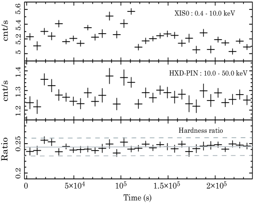
Figure 1.— Energy-resolved light curves of 4U 1626$-$67 observed with Suzaku. Upper and middle panels show background-subtracted light curves obtained with XIS-0 in the 0.4–10.0 keV range and with the HXD in the 10–50 keV range, respectively. The bottom panel shows the hardness ratio of the above two panels.The gray solid line shows the average and the gray dotted lines show the $\pm$3$\sigma$ interval.

3.1. Timing analysis

For the arrival time of each XIS and HXD-PIN event, barycenter correction was performed with the tool aebarycen (Terada et al., 2008). We surveyed the HXD-PIN data by using a folding technique to obtain a best spin period of $P_{(\rm Suzaku)}=7.67795(9)$ s. This period is consistent with the spin-down trend that started to be observed from 1990 onwards, and that is calculated by using the spin-down rate of $\dot{\nu}\sim-4.8\times 10^{-13}$ Hz s^-1 measured with the Swift satellite over the period 2004–2007 (Chakrabarty et al., 1997; Camero-Arranz et al., 2010).

XIS and HXD background-subtracted light curves of 4U 1626$-$67 are shown in Figure 1. The light curves are plotted using a time bin of 7678 s; a multiple of $P_{(\rm Suzaku)}$. The XIS and HXD light curves have an intensity variation of less than 7%, and the hardness ratio between them is approximately constant; the reduced chi-squared ($\chi^{2}$) value is about 1 when fitting a constant model to the hardness ratio. The average and their 3 $\sigma$ level are shown in the Figure 1. As a results, we confirmed that there is no significant spectral variation. Thus, X-ray spectra were extracted by using data over the entire observation.

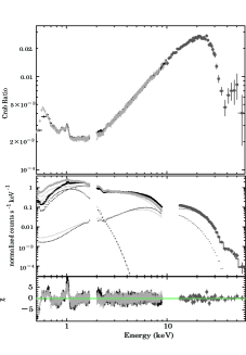
Figure 2.— Phase-averaged background-subtracted spectra of 4U 1626$-$67 obtained with Suzaku XIS (black crosses denote XIS-FI data and light gray crosses denote XIS-BI data) and HXD (denoted by circles). Error bars are only for statistical predictions. The top panel shows the raw count rate energy spectra divided by those of Crab Nebula. The middle panel shows the spectra in counts/s keV^-1 along with the best-fit models (dotted lines) a blackbody, NPEX with Gaussian-absorption model and photoelectric absorption (see text for details). Plots are presented without removal of instrumental responses. The bottom panel shows the residuals between the actual data and the best-fit model.

3.2. Phase-averaged spectrum

The top panel of Figure 2 shows the broadband 4U 1626$-$67 phase-averaged raw count rate spectrum normalized by a Crab Nebula spectrum that was observed for calibration purposes. XIS source data were normalized by using a canonical model of the Crab Nebula spectrum, since spectra from the Crab Nebula suffer from pile-up. HXD data were normalized by a HXD Crab Nebula spectrum observed on 2006 March 30 taken for the same observation parameters—position of the source with respect to the instrument FoV, grade criteria and PIN threshold file (ae_hxd_pinthr_20060727.fits)—as for 4U 1626$-$67. The 4U 1626$-$67 source intensity is about 20 mCrab at 20 keV, and the normalized spectrum is characterized by three main features: a soft X-ray excess below $\sim 3$ keV, as reported by several authors (Angelini et al., 1995; Schulz et al., 2001; Krauss et al., 2007); a power-law continuum and a dip feature at $\sim$35 keV.

To model the phase-averaged spectrum, we fit the data with a $\sim 0.24$ keV blackbody for the soft excess, a negative and positive power-law times exponential (NPEX) model (Mihara, 1995; Makishima et al., 1999) and a Gaussian-absorption (GABS) model (Soong et al., 1990) for the continuum above 3 keV and a standard photoelectric absorption. The NPEX model

$${f(E)=(A_{n}E^{-\alpha}+A_{p}E^{+\beta})\exp\left(-\frac{E}{kT}\right),}$$ (2)

where $E$ is the energy of an incident photon and $kT$ is a plasma temperature (also called the cutoff energy), has two power law components with indices $\alpha$ and $\beta$. The negative $\alpha$ term describes the spectrum at low energy, and the positive $\beta$ term, which dominates as the energy increases, simulates the Wien peak in the unsaturated Comptonization regime when $\beta=2.0$.

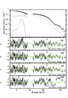
Figure 3.— The top panel shows the phase-averaged and background-subtracted spectra above 3.5 keV of 4U 1626$-$67 obtained with Suzaku XIS (FI: black crosses, BI: light gray crosses) and HXD (gray circles). The lower four panels show the residuals in units of standard deviations, $\chi$, from fitting by: (a) the NPEX with GABS model without Fe-line emission model; (b) the NPEX with GABS model and Fe-line emission model; (c) the NPEX with CYAB and Fe-line emission model and (d) the ECUT with GABS model and Fe-line emission model.

Table 1Best-fit parameters for phase-averaged spectra of 4U 1626$-$67 (d.o.f. = degrees of freedom)

Parameter		NPEX		NPEX with GABS		NPEX with GABS		NPEX with CYAB		ECUT with GABS
$\alpha$		$0.31^{+0.03}_{-0.03}$		$0.26^{+0.02}_{-0.02}$		$0.29^{+0.02}_{-0.02}$		$0.32^{+0.03}_{-0.03}$		$0.65^{+0.06}_{-0.07}$
$kT$(keV)		$5.3^{+0.1}_{-0.1}$		$7.0^{+0.5}_{-0.4}$		$6.7^{+0.2}_{-0.3}$		$7.2^{+1.1}_{-0.4}$		—
$E_{c}$(keV)		—		—		—		—		$24.7^{+0.43}_{-0.53}$
$E_{f}$(keV)		—		—		—		—		$7.08^{+1.14}_{-0.81}$
$A_{n}(\times 10^{-3})$		$8.1^{+0.4}_{-0.3}$		$6.8^{+0.2}_{-0.2}$		$7.2^{+0.3}_{-0.3}$		$7.3^{+0.1}_{-0.3}$		—
$A_{p}(\times 10^{-5})$		$4.6^{+0.3}_{-0.3}$		$1.6^{+0.5}_{-0.4}$		$1.8^{+0.5}_{-0.5}$		$1.6^{+0.4}_{-0.6}$		—
$A(\times 10^{-3})$		—		—		—		—		$10.0^{+1.39}_{-0.75}$
$E_{Fe}$(keV)		—		—		$6.62^{+0.10}_{-0.11}$		$6.60^{+0.10}_{-0.11}$		$6.60$(fix)
$\sigma_{Fe}$(keV)		—		—		$0.37^{+0.13}_{-0.10}$		$0.39^{+0.13}_{-0.10}$		$0.37^{+0.10}_{-0.10}$
$EW_{Fe}$[eV]		—		—		$33.3^{+16.1}_{-16.5}$		$35.2^{+27.7}_{-11.0}$		$31.3^{+3.2}_{-7.6}$
$E_{a}$(keV)		—		$37.6^{+1.02}_{-0.89}$		$37.4^{+1.0}_{-0.9}$		$35.7^{+0.65}_{-0.55}$		$38.4^{+6.47}_{-4.80}$
$\sigma_{CRSF}$(keV)		—		$5.11^{+0.79}_{-0.68}$		$4.99^{+0.71}_{-0.65}$		$5.56^{+1.77}_{-1.08}$		$>16.5$
$\tau$		—		$20.4^{+4.87}_{-4.20}$		$19.0^{+5.0}_{-3.6}$		$25.1^{+3.5}_{-2.3}$		$79.1^{+9.74}_{-4.59}$
$\chi^{2}$ / d.o.f		572.6/158		182.1/155		132.6/152		134.6/152		170.6/152

The best-fit model and its residuals are plotted in the lower panel of Figure 2. Above 3.5 keV only 1% of the NPEX negative term is contributed by the blackbody component. Therefore, hereinafter, we ignore XIS data below 3.5 keV and exclude the blackbody component from the fit.

To evaluate the statistical significance of the CRSF in the phase averaged spectrum, first, we fit the spectrum with only NPEX continuum or NPEX $\times$ GABS model. The residuals of the NPEX with GABS model for energy bands above 3.5 keV are shown in Figure 3(a), and the best-fit parameters are listed in Table 1. Second, we tested the significance using the F-test of Press et al. (2007) routine. In this case, the F statistical value is defined as

$${F=\frac{\chi_{1}^{2}/\nu_{1}}{\chi_{2}^{2}/\nu_{2}},}$$ (3)

where the $\chi_{1}^{2}$ and $\chi_{2}^{2}$ are statistic chi-squared, $\nu_{1}$ and $\nu_{2}$ are degrees of freedom corresponding to the results of fittings using model 1 and model 2 (In this case model 1 is only NPEX continuum and model 2 is NPEX with multiplicative component), respectively. The derived $F$ statistic value is 3.1 which indicates that the probability of chance improvement of the $\chi^{2}$ is $3.7\times 10^{-12}$. Thus, the CRSF is statistically significant feature in the phase averaged spectrum. We also found that the residuals in Figure 3(a) have a complex structure near the Fe-emission line energy around 6.6 keV. The fit improves by the addition of a Gaussian Fe-line model with an energy of 6.62 keV, a width ($\sigma_{Fe}$) of 0.37 keV and an equivalent width (EW) of 33.3 eV (Figure 3(b) and Table 1). These values are statistically consistent with the ASCA EW upper limit of $<33$ eV for an Fe-emission line in the 6.4–6.9 keV range (Angelini et al., 1995). The broad width may indicate the presence an Fe-line complex. If we use three narrow Gaussian Fe-lines, the Fe-line energies are $6.37^{+0.07}_{-0.08}$, $6.61^{+0.05}_{-0.07}$ and $6.92^{+0.04}_{-0.04}$ keV with corresponding EWs of $<11.1$, $<12.2$ and $<17.4$ eV, although the fit is not improved significantly and we would not be distinguish whether the Fe-emission line structure is made by three lines or not, due to the energy resolution of XIS ($\sim$150 eV). The X-ray unabsorbed fluxes in the 3.5–10 keV and 10–60 keV energy bands are $1.27^{+0.01}_{-0.16}\times 10^{-10}$ erg cm^-2 s^-1 and $4.02^{+0.46}_{-0.88}\times 10^{-10}$ erg cm^-2 s^-1, respectively, and the hard X-ray flux is consistent with the BeppoSAX observation (Orlandini et al., 1998). Exchanging the GABS model with a cyclotron absorption model (CYAB; Mihara et al., 1990) also fits the data well (Figure 3(c) and Table 1).

If we replace the NPEX model by an exponential cutoff power-law model (ECUT, which is the powerlaw*highecut model in Xspec; White et al., 1983) and fit the data with a GABS model, we obtain an acceptable $\chi^{2}$ value (see Table 1), but substantial residual structures are seen above 20 keV (Figure 3(d)). Although the CRSF energy agrees with BeppoSAX observations (Orlandini et al., 1998), the best-fit continuum model is inconsistent with BeppoSAX results.

3.3. Phase-resolved spectra

Phase-resolved spectra acquired by HEAO-1, Tenma and RXTE (Pravdo et al., 1979; Kii et al., 1986; Coburn, 2001), show a strong phase dependence in the continuum emission of 4U 1626$-$67. Suzaku XIS and HXD folded light curves also indicate changes across the pulse (Figure 4). Specifically, while the 10–30 keV / 3.5–10 keV ratio maintains the characteristics of the individual light curves, the 30–50 keV / 10–30 keV ratio indicates spectral differences between phases 0.0–0.3 and the other phases. To investigate spectral changes across the pulse, we divided the events into eight phase-resolved spectra (Figure 5) and normalized these spectra by the Crab Nebula spectrum by using the method described in §3.2 (Figure 6). The Crab Ratios show that the $\sim 20$ keV peak is more prominent at higher pulse flux. Additionally, the Ratios flatten at lower pulse flux and the energy of resonance feature changes. The resonance features are particularly outstanding in the dim phase spectrum ($\phi=0.125$–0.250), where the hardness ratio (Figure 4) shows the large change in these features.

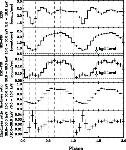
Figure 4.— Energy-resolved and background-inclusive pulse profiles of 4U 1626$-$67. Data were folded at $P_{(\rm Suzaku)}=7.67795$ s. Phase 0 corresponds to MJD 53803.000092755. The average background count rates of 3.5–10.0 keV, 10.0–30.0 keV and 30.0–50.0 keV energy bands are 0.016 counts/s, 0.49 counts/s and 0.086 counts/s, respectively.

Table 2NPEX continuum-only best-fit parameters for phase resolved spectra of 4U 1626$-$67.

pulse	$\alpha$	kT	$A_{n}$	$A_{p}$	EWFe	$\chi^{2}$ / d.o.f
phase		(keV)	$(\times 10^{-3})$	$(\times 10^{-5})$	(eV)
0.000–0.125	$-0.02^{+0.05}_{-0.06}$	$4.4^{+0.4}_{-0.3}$	$6.7^{+0.8}_{-0.7}$	$3.2^{+2.3}_{-1.9}$	$27^{+38}_{-2}$	81.2 / 81
0.125–0.250	$0.15^{+0.17}_{-0.11}$	$5.1^{+0.7}_{-1.1}$	$5.8^{+0.7}_{-0.5}$	$<1.2$	$81^{+28}_{-12}$	69.0 / 63
0.125–0.250	$0.27^{+0.02}_{-0.02}$	$6.1^{+0.5}_{-0.4}$	$6.1^{+0.2}_{-0.2}$	0 (fixed)	$84^{+13}_{-53}$	71.8 / 64
0.250–0.375	$0.10^{+0.07}_{-0.06}$	$4.3^{+0.2}_{-0.3}$	$8.04^{+1.3}_{-0.7}$	$4.9^{+2.5}_{-1.7}$	$46^{+31}_{-8}$	93.4 / 97
0.375–0.500	$0.51^{+0.11}_{-0.06}$	$5.0^{+0.1}_{-0.1}$	$11.8^{+1.9}_{-0.8}$	$7.6^{+1.1}_{-0.7}$	$21^{+16}_{-9}$	137.3 / 103
0.500–0.625	$0.56^{+0.10}_{-0.10}$	$5.3^{+0.1}_{-0.1}$	$10.4^{+1.6}_{-1.3}$	$7.2^{+0.6}_{-0.6}$	$<22$	297.9 / 129
0.625–0.750	$0.64^{+0.10}_{-0.09}$	$5.2^{+0.1}_{-0.1}$	$11.8^{+1.7}_{-1.5}$	$8.4^{+0.7}_{-0.7}$	$35^{+5}_{-10}$	259.0 / 108
0.750–0.875	$0.53^{+0.09}_{-0.09}$	$5.3^{+0.1}_{-0.1}$	$9.8^{+1.4}_{-1.2}$	$7.5^{+0.7}_{-0.7}$	$35^{+17}_{-15}$	247.2 / 91
0.875–1.000	$0.45^{+0.07}_{-0.07}$	$5.3^{+0.2}_{-0.1}$	$9.9^{+1.08}_{-0.9}$	$5.7^{+0.7}_{0.7}$	$31^{+33}_{-27}$	117.5/ 89

Table 3Best-fit parameters for phase resolved spectra of 4U 1626$-$67, when fitting by NPEX with GABS model

pulse	$\alpha$	kT	$A_{n}$	$A_{p}$	$E_{a}$	$\sigma_{CRSF}$	$\tau$	EWFe	$\chi^{2}$ / d.o.f	$F$/PCI
phase		(keV)	$(\times 10^{-3})$	$(\times 10^{-5})$	(keV)	(keV)		(eV)
0.000–0.125	$0.05^{+0.18}_{-0.07}$	$5.4^{+1.8}_{-0.8}$	$6.5^{+0.5}_{-0.4}$	$<2.4$	$31.3^{+2.3}_{-1.6}$	$0.5^{+2.5}_{-0.3}$	$>5$	$<57$	66.9 / 78	1.169/$2.45\times 10^{-1}$
0.125–0.250	$0.29^{+0.26}_{-0.40}$	$11.2^{+4.4}_{-1.8}$	$7.8^{+10.8}_{-1.7}$	0 (fixed)	$26.3^{+5.6}_{-4.1}$	$>9.1$	$66^{+94}_{-42}$	$69^{+46}_{-35}$	52.0 / 61	1.316/$1.41\times 10^{-1}$
0.250–0.375	$0.21^{+0.29}_{-0.22}$	$6.5^{+2.6}_{-3.0}$	$7.5^{+1.0}_{-0.5}$	$<4.6$	$33.5^{+8.1}_{-3.2}$	$4.5^{+4.7}_{-1.2}$	$15^{+47}_{-8}$	$43^{+23}_{-28}$	85.3 / 94	1.061/$3.87\times 10^{-1}$
0.375–0.500	$0.40^{+0.07}_{-0.07}$	$5.6^{+0.6}_{-0.2}$	$9.8^{+1.2}_{-1.9}$	$5.0^{+1.1}_{-2.0}$	$37.1^{+3.8}_{-0.9}$	$4.0^{+2.8}_{-1.5}$	$14^{+15}_{-6.0}$	$24^{+37}_{-7}$	91.9 / 100	1.451/$3.14\times 10^{-2}$
0.500–0.625	$0.33^{+0.07}_{-0.07}$	$6.6^{+0.5}_{-0.4}$	$6.8^{+0.9}_{-0.8}$	$3.4^{+0.9}_{-1.0}$	$37.2^{+2.2}_{-1.2}$	$3.9^{+1.2}_{-1.1}$	$22^{+11}_{-6}$	$<45$	133.6 / 126	2.178/$7.62\times 10^{-6}$
0.625–0.750	$0.38^{+0.02}_{-0.03}$	$6.4^{+0.1}_{-0.1}$	$8.0^{+0.1}_{-0.1}$	$4.2^{+0.5}_{-0.1}$	$36.8^{+1.0}_{-0.9}$	$4.0^{+1.1}_{-0.8}$	$20^{+4}_{-3}$	$39^{+6}_{-19}$	83.6 / 105	3.012/$1.63\times 10^{-8}$
0.750–0.875	$0.27^{+0.05}_{-0.06}$	$7.1^{+0.8}_{-0.5}$	$6.7^{+0.7}_{-0.7}$	$2.6^{+1.0}_{-1.2}$	$39.0^{+2.5}_{-1.9}$	$5.5^{+1.4}_{-1.2}$	$29^{+29}_{-9}$	$38^{+26}_{-22}$	108.7 / 88	2.199/$1.25\times 10^{-4}$
0.875–1.000	$0.37^{+0.15}_{-0.07}$	$8.0^{+20.0}_{-2.5}$	$7.6^{+0.8}_{-0.5}$	$1.4^{+3.0}_{-0.7}$	$43.3^{+9.4}_{-8.5}$	$10.0^{+4.6}_{-3.2}$	$>10$	$30^{+28}_{-25}$	90.4/ 86	1.256/$1.45\times 10^{-1}$

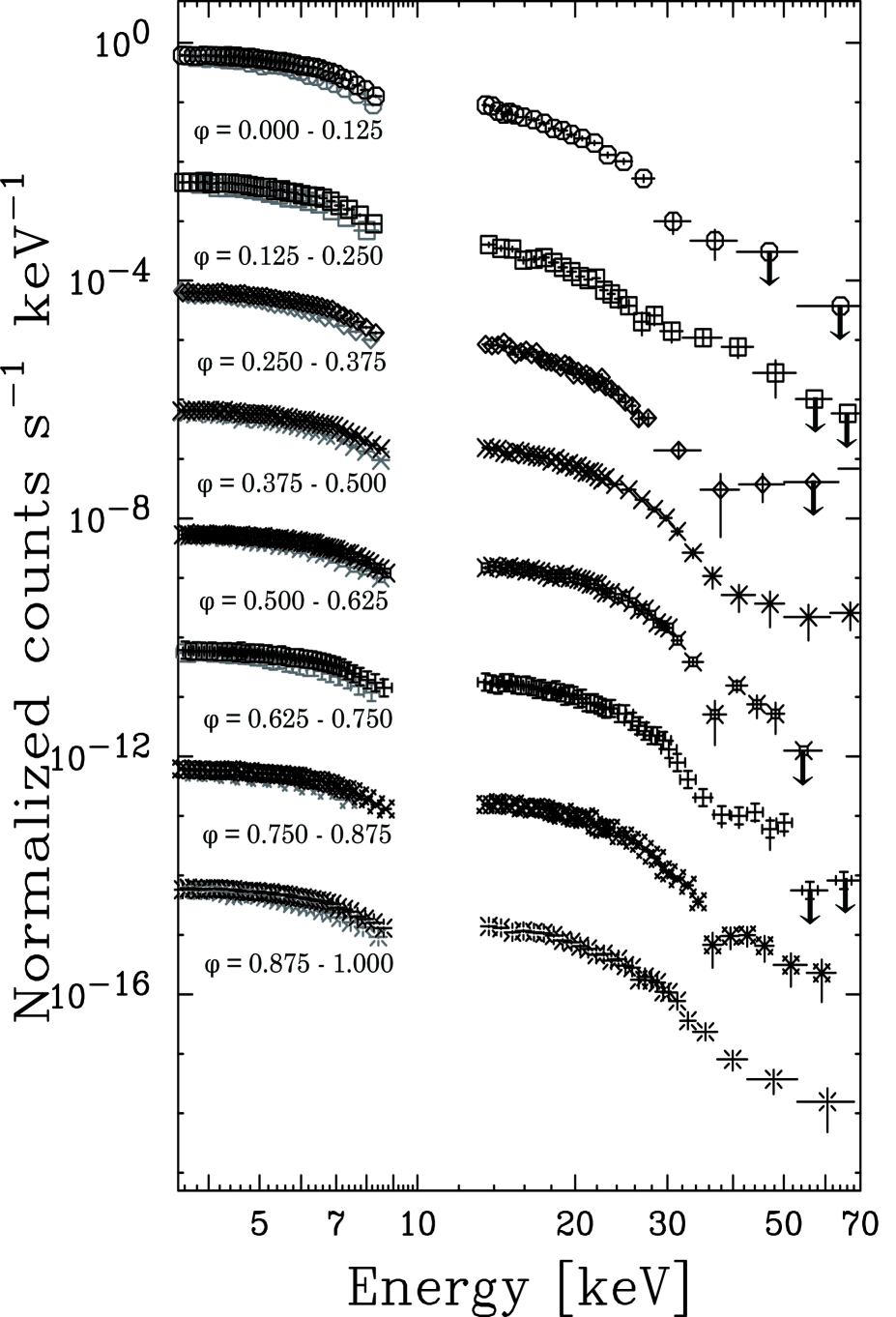
Figure 5.— Phase-resolved and background-subtracted XIS (FI: black symbols below 10 keV, BI: gray symbols) and HXD (black symbols over 10 keV) spectra of 4U 1626$-$67 for phases $\phi=0.000$–0.125, 0.125–0.250, 0.250–0.375, 0.375–0.500, 0.500–0.625, 0.625–0.750, 0.750–0.875 and 0.875–1.000 from top to bottom, offset by multiples of $10^{-2}$. Arrows denote the upper limit.

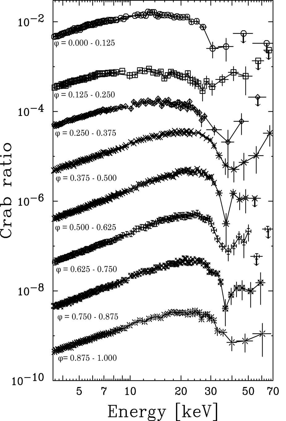
Figure 6.— Ratios between the phase-resolved and background-subtracted XIS and HXD spectra of 4U 1626$-$67 and those of the Crab Nebula. The XIS source data were normalized using the canonical model of the Crab Nebula since spectra from the Crab Nebula suffer from pile-up. Phases are indicated in the same manner as Figure 5, but are offset by multiples of $10^{-1}$. Arrows denote the upper limit.

We then performed spectral fitting to the phase-resolved spectra with the NPEX continuum and the Fe-emission line model in order to establish the pulse-phase dependence of the continuum and the CRSF. The Fe-line energy and the width of the Gaussian function were fixed at values obtained from the averaged spectrum. The parameters from the spectral fitting are listed in Table 2, and the ratios between the original data and the best-fit model are shown in Figure 7. We found that the ratio for the dim phase ($\phi=0.125$–0.250) spectrum exhibits a monotone increase above 30 keV, and the residuals show evidence for the existence of an emission feature rather than an absorption (Figure 8(a)). In contrast, the other phases have a V-shaped ratio caused by a CRSF absorption feature. Moreover, the fitting results for the dim phase spectrum show that the $A_{p}$ parameter is unconstrained, strongly suggesting that the continuum spectrum at the dim phase requires only the upper limit of the high-energy cutoff component. In other words, the result make the NPEX model effectively a power-law times exponential cutoff model (cutoffpl in Xspec). The result is consistent with the trend that the 20 keV peak in the Crab Ratios is less prominent at lower pulse flux. We also tried other empirical models applied to accretion powered pulsar, ECUT and a powerlaw with Fermi-Dirac cutoff (FDCO; Tanaka, 1986), and find that their best fit cutoff energies are consistent with 0. In other words, a power-law times an exponential cutoff model is the only one able to fit the dim phase spectrum. For this reason we fit the dim phase spectrum by using the NPEX model with fixed $A_{p}=0$. As we can see in Table 2, the difference between the $\chi^{2}$ values for freely selected $A_{p}$ and for fixed $A_{p}=0$ is negligible. Therefore, we henceforth fix $A_{p}=0$ for the NPEX model when fitting the dim phase spectrum.

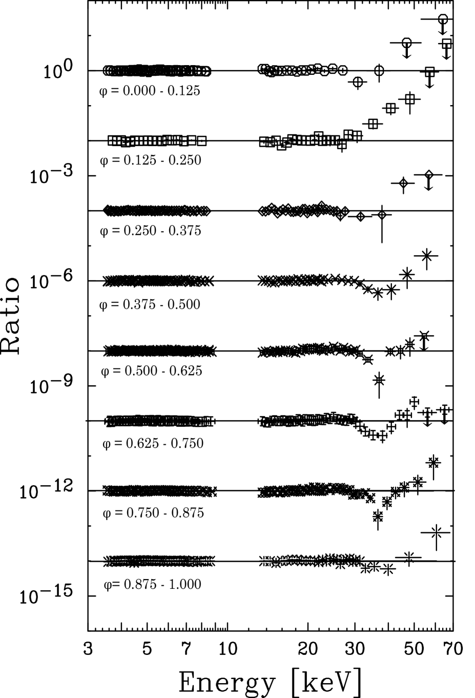
Figure 7.— Ratios between the data and best-fit NPEX-only model for each phase-resolved spectra. Phases are indicated in the same manner as Figure 5. Arrows denote the upper limit.

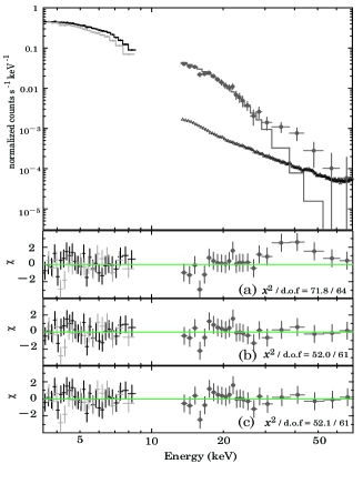
Figure 8.— Upper panel shows spectra in the dim phase ($\phi=0.125$–0.250) of 4U 1626$-$67 obtained with Suzaku XIS (FI: black crosses, BI: light gray crosses) and HXD (circles). Triangles denote the reproducibility of NXB for HXD-PIN. Histograms in the upper panel are the best-fit by NPEX continuum ($A_{p}=0$). The lower three panels show residuals, $\chi$, when fitting by (a) NPEX ($A_{p}=0$) continuum-only; (b) NPEX ($A_{p}=0$) with GABS model and (c) NPEX ($A_{p}=0$) and Gaussian models.

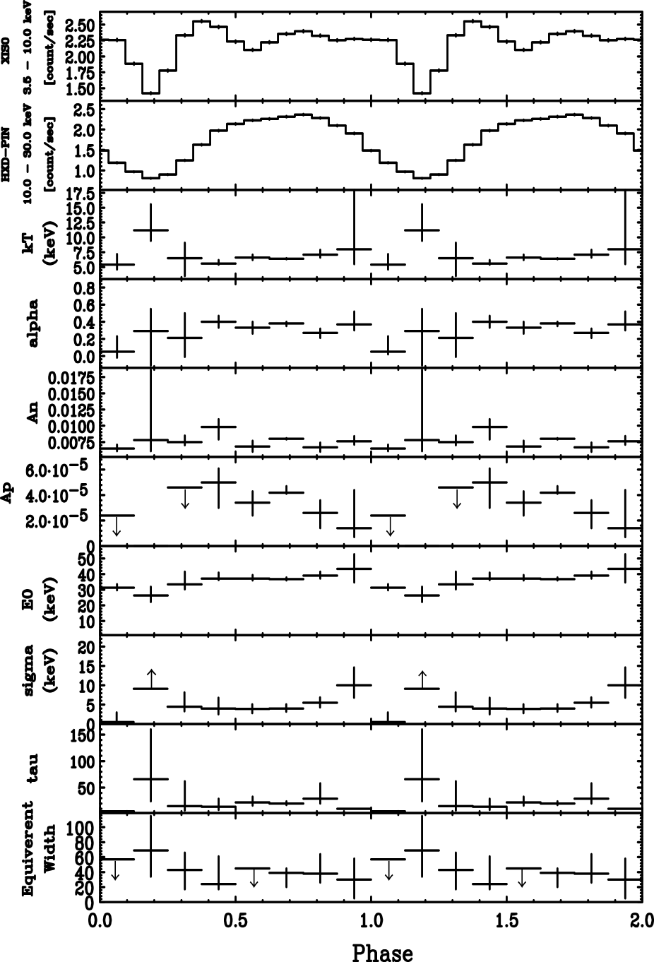
Figure 9.— Fit parameters from as a function of pulse phase for 4U 1626$-$67. Best-fit values by NPEX with GABS model (Table 3) are plotted.

Next, we included the GABS model and refit the phase-resolved spectra. The resulting parametrized models fit all of the phase-resolved spectra well (see Table 3 and Figure 9), and residuals above 30 keV in the dim phase were eliminated (see Figure 8(b)). We also evaluate the significance of including a GABS component using the same method discussed in section 3.1. The derived probabilities are summarized in Table 3, that shows that the absorption factor is not statistically significant in the dim phase. This significance did not change even when we adopted the CYAB model (as opposed to the GABS model as the cyclotron feature model) for spectral fitting.

Table 4Best-fit parameters for phase resolved spectra of 4U 1626$-$67, when fitting by NPEX plus Gaussian model.

pulse	$\alpha$	kT	$A_{n}$	$A_{p}$	$E_{a}$	$\sigma_{CRSF}$	Norm	EWFe	$\chi^{2}$ / d.o.f	$F$/PCI
phase		(keV)	$(\times 10^{-3})$	$(\times 10^{-5})$	(keV)	(keV)	$(\times 10^{-4})$	(eV)
0.000–0.125	$0.04^{+0.19}_{-0.08}$	$5.3^{+1.8}_{-0.8}$	$6.5^{+0.5}_{-0.4}$	$<3.1$	$30.8^{+1.8}_{-1.4}$	$<3.4$	$-2.3^{+1.1}_{-1.6}$	$27^{+16}_{-10}$	66.8 / 78	5.617/ 1.54$\times 10^{-3}$
0.125–0.250	$0.15^{+0.14}_{-0.17}$	$5.4^{+0.4}_{-0.8}$	$5.5^{+0.8}_{-0.7}$	$0$(fixed)	$40.5^{+13.7}_{-14.7}$	$>4.5$	$8.8^{+7.2}_{-2.9}$	$71^{+29}_{-36}$	52.1 / 61	7.688/1.94$\times 10^{-4}$
0.250–0.375	$0.21^{+0.20}_{-0.15}$	$6.3^{+2.2}_{-1.9}$	$7.6^{+0.5}_{-0.6}$	$<4.5$	$29.9^{+2.7}_{-5.6}$	$5.4^{+4.6}_{-4.9}$	$-6.7^{+5.6}_{-17.4}$	$47^{+17}_{-17}$	85.2 / 94	3.028/3.33$\times 10^{-2}$
0.375–0.500	$0.39^{+0.09}_{-0.08}$	$5.7^{+2.6}_{-0.4}$	$9.6^{+1.5}_{-1.3}$	$4.5^{+1.5}_{-2.8}$	$34.2^{+1.4}_{-5.7}$	$4.9^{+8.0}_{-1.9}$	$-11.9^{+5.2}_{-90.3}$	$25^{+23}_{-3}$	91.8 / 100	16.511/8.65$\times 10^{-9}$
0.500–0.625	$0.33^{+0.08}_{-0.07}$	$6.6^{+0.5}_{-0.4}$	$6.8^{+0.9}_{-0.7}$	$3.4^{+0.9}_{-0.8}$	$34.8^{+0.6}_{-0.6}$	$4.4^{+1.2}_{-1.1}$	$-22.9^{+6.3}_{-9.6}$	$<31$	131.4 / 126	53.190/2.78$\times 10^{-22}$
0.625–0.750	$0.37^{+0.08}_{-0.07}$	$6.5^{+0.5}_{-0.4}$	$7.9^{+0.1}_{-0.1}$	$3.9^{+0.9}_{-0.8}$	$34.2^{+0.6}_{-0.6}$	$4.7^{+1.2}_{-1.0}$	$-25.7^{+6.7}_{-10.2}$	$39^{+5}_{-16}$	85.0 / 105	71.710/ 2.60$\times 10^{-25}$
0.750–0.875	$0.28^{+0.06}_{-0.06}$	$7.0^{+0.8}_{-0.6}$	$6.8^{+0.8}_{-0.6}$	$2.8^{+1.0}_{-0.8}$	$34.7^{+0.7}_{-0.7}$	$5.9^{+1.7}_{-1.2}$	$-31.5^{+10.2}_{-19.0}$	$37^{+7}_{-23}$	109.8 / 88	36.737/1.73$\times 10^{-15}$
0.875–1.000	$0.38^{+0.08}_{-0.08}$	$7.6^{+2.2}_{-1.3}$	$7.8^{+0.8}_{-0.7}$	$1.8^{+1.2}_{-0.7}$	$32.0^{+3.6}_{-16.4}$	$10.2^{+8.6}_{-6.0}$	$-48.5^{+61.5}_{-52.4}$	$31^{+35}_{-5}$	89.2/ 86	9.099/ 2.70$\times 10^{-5}$

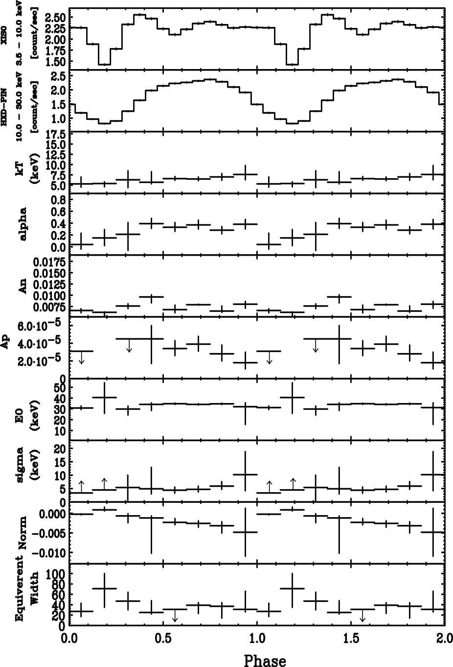
Figure 10.— Fit parameters from as a function of pulse phase for 4U 1626$-$67. Best-fit values by NPEX plus Gaussian model (Table 4) are plotted.

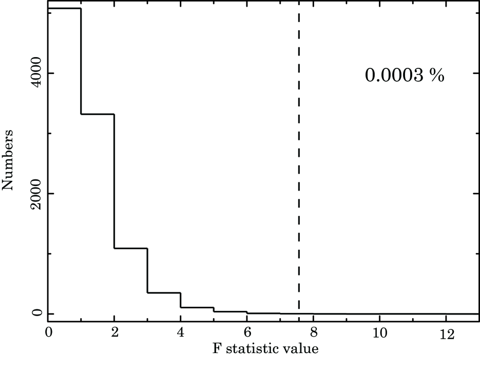
Figure 11.— Observed value of the $F_{\chi}$ plotted as dashed line against probability histogram of $F_{\chi}$ obtained by 10,000 simulations (See the text).

Since the GABS model reproduces an absorption feature, we fit the phase-resolved spectra by the NPEX plus a Gaussian model in which we allowed the Gaussian normalization to be both positive and negative. The derived parameters are shown at Table 4 and Figure 10. The results indicates that the emission line produces the residuals from the NPEX fitting in Figure 8(a). We can evaluate how much the additional term improved the fit using the F-test for additional terms (Bevington, 1969). The F statistical value, hereafter called F_χ, is defined as

$${F_{\chi}=\frac{(\chi_{1}^{2}-\chi_{2}^{2})/(\nu_{2}-\nu_{1})}{\chi_{2}^{2}/\nu_{2}}.}$$ (4)

Each suffix denotes model 1 and 2, NPEX only and NPEX + Gaussian model, respectively. The derived probability from $F_{\chi}$ also summarized at Table 5. The results show that the data support the presence of the emission line in the dim phase with $F_{\chi}$ of 7.688, corresponding to a probability of chance improvement of the $\chi^{2}$ of 1.9 $\times$ 10^-4. The residuals of the fitting are shown in Figure 8(c). The obtained resonance energy, $E_{a}=40.5^{+13.7}_{-14.7}$ keV, is statistically consistent with those observed in the other phases.

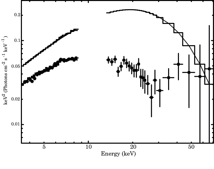
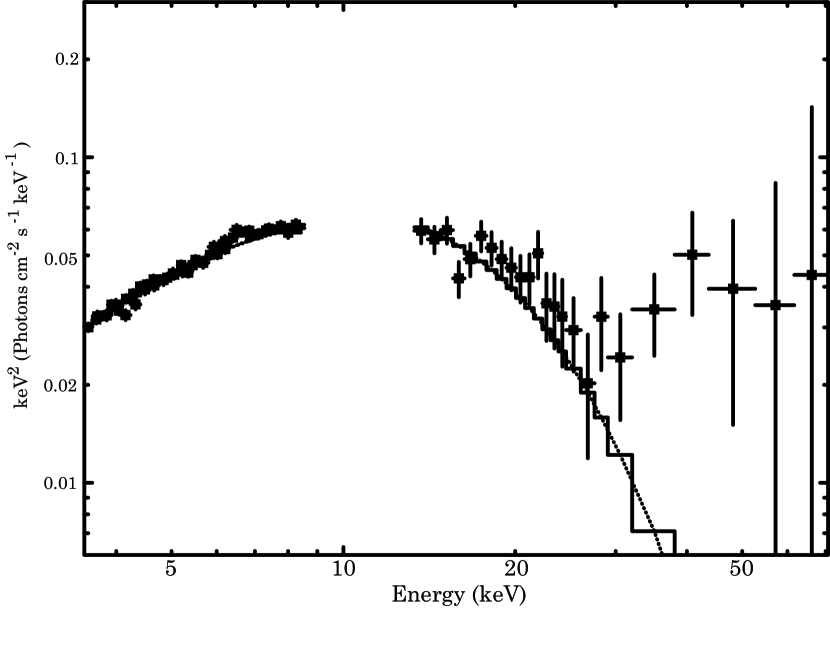
Figure 12.— The dim phase $\nu F\nu$ spectra of the 4U 1626$-$67 obtained with XIS and HXD. The NPEX-only ($A_{p}$ = 0) models are shown in the histogram. (Left) When fitted by NPEX ($A_{p}$ = 0) with GABS model and (right) when fitted by NPEX ($A_{p}$ = 0) and Gaussian models.

To examine the chance probability of improvement of the derived F-value, we simulate the spectra following a procedure similar to section 5.2 of Protassov et al. (2002). First, we simulate 10,000 data sets using ”fakeit” in XSPEC Version12 according to the NPEX ($A_{p}=0$) model with parameters fixed at best fit values listed in Table 2, same instrumental response, background files and same exposure time. Each data set is binned using same binning as that used to real data. Second, we fit the simulate data using only NPEX ($A_{p}=0$) and NPEX ($A_{p}=0$) + Gaussian model allowing their normalization to be negative. Third, we calculate the $F_{\chi}$ derived by these two model fittings. Last, we evaluated the number of simulated spectra with $F_{\chi}$ exceeding the 7.688, which is derived by fitting of real data to estimate the approximate probability. The derived histogram of the $F_{\chi}$ is shown at Figure 11 and the evaluated chance probability is 3.0 $\times$ 10^-4 which is consistent with the $F_{\chi}$ value obtained from real data using equation (4). In order to evaluate the effect of systematic error of HXD-PIN non-X-ray-background model, we also refit the dim phase spectrum taking account into the 3 % systematic errors of HXD-PIN. The $F_{\chi}$ is $7.688^{+2.523}_{-2.490}$ and the probability is between $2.91\times 10^{-3}$and $1.53\times 10^{-5}$. Therefore, even though the NXB level of HXD-PIN is underestimated, we have possibly detected the emission line at the cyclotron resonance energy in the dim phase. Although there is a $\sim$ 85 % possibility that the structure in the dim phase is produced by absorption feature, we stress that the continuum requires a hard component with a large cutoff energy, in addition to a wide and deep absorption feature, as seen in Figure 12. Furthermore, the $kT$ value at the dim phase matches those at the other phases with the emission model, whereas a large jump in the value is required with the absorption model, as shown in Figure 9.

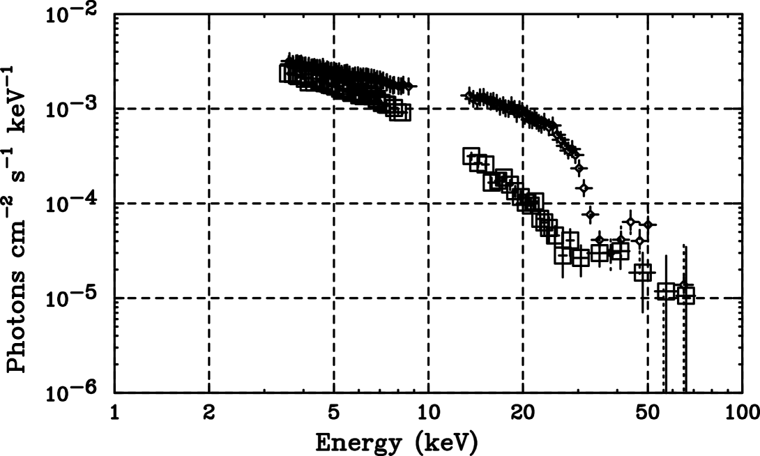
Figure 13.— The unfolded spectrum of 4U 1626$-$67. Crosses denote on-phase spectra ($\phi=0.625$–0.750). Squares denote off-phase spectra ($\phi=0.125$–0.250).

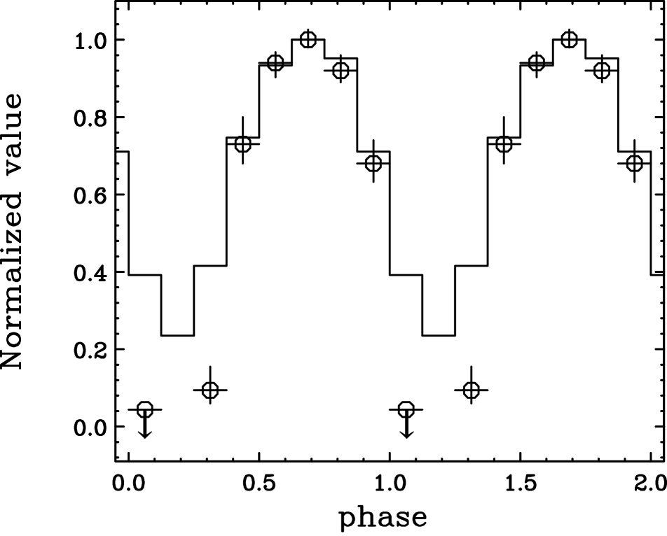
Figure 14.— The plotted line is the background-subtracted pulse profile in the 10–30 keV energy band. The circles denote the best-fit values of the normalization of the positive power-law term (i.e., the Wien hump) when fitting by NPEX model, presented as a function of the pulse phase (see text for details). Values are normalized by each maximum value.

4. Discussion

We observed the 4U 1626$-$67 pulsar with the Suzaku satellite in March 2006. The pulse period determined by the HXD-PIN of Suzaku is $P_{(\rm Suzaku)}$ = $7.67795(9)$ s, and this value agrees with that reported by Camero-Arranz et al. (2010). In the pulse phase-averaged spectra, the fundamental CRSF is clearly detected at $37.4^{+1.0}_{-0.9}$ keV (GABS model) and the continuum emission is better reproduced by the NPEX model than the ECUT model. Phase-resolved spectral analyses consistently show strong phase dependence, both in the continuum emission and in the CRSF, particularly in the dim phase. Quantitatively, the positive component of the NPEX model vanishes near the dim phase, and the CRSF in the dim phase is reproduced by using a Gaussian shaped emission line model. The statistical significance of the emission line using the Bevington (1969) F-test routine is $2.91\times 10^{-3}$ and $1.53\times 10^{-5}$ taking account into the systematic errors in the background evaluation of HXD-PIN. The results means that even if the the real NXB level of HXD-PIN is 3% higher, which is the worst case of underestimating NXB level, the significance level is still around 3$\sigma$ level. Thus, we have possibly detected the emission line at the cyclotron resonance energy in the dim phase.

In this section, we discuss the nature of the accretion column on the magnetic pole of the neutron star that produces a cyclotron emission line at the dim phase rather than an absorption feature.

What is the origin of the emission feature in the dim phase? Nagel (1981) pointed out that if the photons originate from an optically thick accretion column (with a Thomson optical depth $\tau_{T}>1$) without temperature and density gradients, the CRSF is expected to be an absorption feature with Comptonized spectra. In contrast, if the photons originate from an optically thin accretion column ($\tau_{T}<1$), the CRSF is expected to be an emission feature with a free-free continuum. To compare this theoretical model with the Suzaku spectra, the unfolded spectra in the on-phase ($\phi=0.625$–0.750) and the dim phase ($\phi=0.125$–0.250) are shown in Figure 13. Qualitatively, our observed results are consistent with the theoretical predictions; the Wien hump disappears with the appearance of an emission-like feature. This resemblance suggests that we observed the cyclotron resonance scattering emission feature caused by collisional excitation of a Landau level, followed by radiative deexcitation. The deciding factor as to whether we observe absorption spectra or emission spectra is thus the optical depth of the accretion column, and for the case of 4U 1626$-$67, since change occurs according to the spin phase, changes in optical depth arise from changes in viewing angle.

The optical depth, $\tau$, is generally expressed as

$${\tau=n_{e}\sigma l.}$$ (5)

Here, $n_{e}$ is the electron number density, $\sigma$ is the scattering cross section and $l$ is the plasma length-scale through which a photon passes. In a strong magnetic field, where the strength of the field is greater than the thermal energy, the scattering cross section depends on the direction of photons relative to the magnetic field vector. According to Herold (1979), the scattering cross section of photons averaged over the energy and the (ordinary and extraordinary) modes is described by

$${\sigma_{\parallel}\approx\sigma_{T}\biggl{(}\frac{\bar{E}}{E_{a}}\biggr{)}^{2},}$$ (6)

when the photons have energies far less than $E_{a}$, and they propagate parallel to the magnetic field. Here, $\sigma_{T}$ is the Thomson scattering cross section and $\bar{E}$ is the mean photon energy. Thus, the optical depth propagating parallel to the magnetic field, $\tau_{\parallel}$, is

$${\tau_{\parallel}\approx n_{e}\sigma_{T}\biggl{(}\frac{\bar{E}}{E_{a}}\biggr{)}^{2}l_{\parallel}.}$$ (7)

In contrast, the averaged cross section for photons propagating perpendicular to the magnetic field, $\sigma_{\perp}$, can be approximated by

$${\sigma_{\perp}\approx\sigma_{T},}$$ (8)

and the optical depth propagating perpendicular to the magnetic field, $\tau_{\perp}$, is

$${\tau_{\perp}\approx n_{e}\sigma_{T}l_{\perp}.}$$ (9)

Therefore, from equations (7) and (9) we see that the optical depth is anisotropic, and the probability of Comptonization of photons depends on the direction that the photons are propagating through the plasma. This anisotropy of optical depth in the Comptonization process is expected to cause the phase dependence of the Wien hump.

To verify the phase dependence of the Wien hump, we again fit the phase-resolved spectra by the NPEX model, except for the dim phase, where the $kT$ value are instead fixed at the phase-averaged value (Table 1) by assuming thermal equilibrium. Here, the CRSF is described by the GABS model and the spectral fits are found to be acceptable. Figure 14 shows the background-subtracted pulse profile for the 10–30 keV energy band and compares this with values of $A_{p}$ plotted as a function of the pulse phase. These two plots clearly agree. In other words, X-ray fluxes in the 10–30 keV range are represented by only the Wien hump. Since, as described above, radiation is caused by the optical depth of scattering, the dim phase corresponds to the optically thin phase. Therefore, this result is explained correctly by our prediction.

To estimate the value of $\tau_{\parallel}$ qualitatively, we use the simple assumptions that the plasma is at thermal equilibrium and that the accretion column is homogeneous. Under these conditions, $\bar{E}$ is equal to the electron temperature. Therefore, the ratio between $\tau_{\parallel}$ and $\tau_{\perp}$ is estimated by using the observed $kT\sim 6.71$ keV and the $E_{a}\sim 37.4$ keV derived from fitting the phase-averaged spectra by the NPEX with GABS model (Table 1):

$$\frac{\tau_{\parallel}}{\tau_{\perp}}\approx\biggl{(}\frac{\bar{E}}{E_{a}}\biggr{)}^{2}\frac{l_{\parallel}}{l_{\perp}}\approx\biggl{(}\frac{kT}{E_{a}}\biggr{)}^{2}\frac{l_{\parallel}}{l_{\perp}}=3.2\times 10^{-2}\frac{l_{\parallel}}{l_{\perp}}.$$ (10)

Thus, if the difference between $l_{\parallel}$ and $l_{\perp}$ is small ($l_{\parallel}\sim l_{\perp}$), the optical depth for the dim phase spectra is approximately one or two orders of magnitude lower than that in the bright phase. If we assume that the Thomson optical depth of the bright phase is around 10, the cyclotron resonance scattering absorption feature can be seen as an emission feature at a certain viewing angle.

In the future, we plan to further investigate the radiative transfer of photons in the accretion column through theoretical studies that take into account emission power.

The authors appreciate very much the many constructive comments from the anonymous referee. We thank all of the Suzaku team members for their dedicated support in the satellite operation and calibration. W.B.Iwakiri is a Research Fellow of the Japan Society for the Promotion of Science (JSPS).

References

- Angelini et al. (1995) Angelini, L., White, N. E., Nagase, F., et al. 1995, ApJ, 449, L41
- Bevington (1969) Bevington, P. R. 1969, New York: McGraw-Hill, 1969,
- Boldt (1987) Boldt, E. 1987, Observational Cosmology, 124, 611
- Camero-Arranz et al. (2010) Camero-Arranz, A., Finger, M. H., Ikhsanov, N. R., Wilson-Hodge, C. A., & Beklen, E. 2010, ApJ, 708, 1500
- Chakrabarty et al. (1997) Chakrabarty, D., Bildsten, L., Grunsfeld, J. M., et al. 1997, ApJ, 474, 414
- Chakrabarty (1998) Chakrabarty, D. 1998, ApJ, 492, 342
- Coburn (2001) Coburn, W. 2001, Ph.D. Thesis,
- Coburn et al. (2002) Coburn, W., Heindl, W. A., Rothschild, R. E., et al. 2002, ApJ, 580, 394
- Enoto et al. (2008) Enoto, T., Makishima, K., Terada, Y., et al. 2008, PASJ, 60, 57
- Fukazawa et al. (2009) Fukazawa, Y., Mizuno, T., Watanabe, S., et al. 2009, PASJ, 61, 17
- Herold (1979) Herold, H. 1979, Phys. Rev. D, 19, 2868
- Kii et al. (1986) Kii, T., Hayakawa, S., Nagase, F., Ikegami, T., & Kawai, N. 1986, PASJ, 38, 751
- Koyama et al. (2007) Koyama, K., Tsunemi, H., Dotani, T., et al. 2007, PASJ, 59, 23
- Krauss et al. (2007) Krauss, M. I., Schulz, N. S., Chakrabarty, D., Juett, A. M., & Cottam, J. 2007, ApJ, 660, 605
- Makishima et al. (1999) Makishima, K., Mihara, T., Nagase, F., & Tanaka, Y. 1999, ApJ, 525, 978
- Middleditch et al. (1981) Middleditch, J., Mason, K. O., Nelson, J. E., & White, N. E. 1981, ApJ, 244, 1001
- Mihara et al. (1990) Mihara, T., Makishima, K., Ohashi, T., Sakao, T., & Tashiro, M. 1990, Nature, 346, 250
- Mihara (1995) Mihara, T. 1995, Ph.D. Thesis,
- Mitsuda et al. (2007) Mitsuda, K., Bautz, M., Inoue, H., et al. 2007, PASJ, 59, 1
- Nagel (1981) Nagel, W. 1981, ApJ, 251, 288
- Orlandini et al. (1998) Orlandini, M., Fiume, D. D., Frontera, F., et al. 1998, ApJ, 500, L163
- Pravdo et al. (1979) Pravdo, S. H., White, N. E., Boldt, E. A., et al. 1979, ApJ, 231, 912
- Press et al. (2007) Press, WH; Teukolsky, SA; Vetterling, WT; Flannery, BP (2007), ”Section 14.2.2. F-Test for Significantly Different Variances”, Numerical Recipes: The Art of Scientific Computing (3rd ed.), New York: Cambridge University Press, ISBN 978-0-521-88068-8
- Protassov et al. (2002) Protassov, R., van Dyk, D. A., Connors, A., Kashyap, V. L., & Siemiginowska, A. 2002, ApJ, 571, 545
- Rivers et al. (2010) Rivers, E., Markowitz, A., Pottschmidt, K., et al. 2010, ApJ, 709, 179
- Schulz et al. (2001) Schulz, N. S., Chakrabarty, D., Marshall, H. L., Canizares, C. R., Lee, J. C., & Houck, J. 2001, ApJ, 563, 941
- Serlemitsos et al. (2007) Serlemitsos, P. J., Soong, Y., Chan, K.-W., et al. 2007, PASJ, 59, 9
- Soong et al. (1990) Soong, Y., Gruber, D. E., Peterson, L. E., & Rothschild, R. E. 1990, ApJ, 348, 641
- Suchy et al. (2011) Suchy, S., Pottschmidt, K., Rothschild, R. E., et al. 2011, ApJ, 733, 15
- Sunyaev & Titarchuk (1980) Sunyaev, R. A., & Titarchuk, L. G. 1980, A&A, 86, 121
- Takahashi et al. (2007) Takahashi, T., Abe, K., Endo, M., et al. 2007, PASJ, 59, 35
- Tanaka (1986) Tanaka, Y. 1986, IAU Colloq. 89: Radiation Hydrodynamics in Stars and Compact Objects, 255, 198
- Terada et al. (2006) Terada, Y., Mihara, T., Nakajima, M., et al. 2006, ApJ, 648, L139
- Terada et al. (2008) Terada, Y., Enoto, T., Miyawaki, R., et al. 2008, PASJ, 60, 25
- Trümper et al. (1978) Trümper, J., Pietsch, W., Reppin, C., Voges, W., Staubert, R., & Kendziorra, E. 1978, ApJ, 219, L105
- White et al. (1983) White, N. E., Swank, J. H., & Holt, S. S. 1983, ApJ, 270, 711
- Yamamoto et al. (2011) Yamamoto, T., Sugizaki, M., Mihara, T., et al. 2011, PASJ, 63, 751