Two-component solitons under a spatially modulated linear coupling: Inverted photonic crystals and fused couplers

Abstract

We study two-component solitons and their symmetry-breaking bifurcations (SBBs) in linearly coupled photonic systems with a spatially inhomogeneous strength of the coupling. One system models an inverted virtual photonic crystal, built by periodically doping the host medium with atoms implementing the electromagnetically induced transparency (EIT). In this system, two soliton-forming probe beams with different carrier frequencies are mutually coupled by the EIT-induced effective linear interconversion. The system is described by coupled nonlinear Schrödinger (NLS) equations for the probes, with the linear-coupling constant periodically modulated in space according to the density distribution of the active atoms. The type of the SBB changes from sub- to supercritical with the increase of the total power of the probe beams, which does not occur in systems with constant linear-coupling constants. Qualitatively similar results for the SBB of two-component solitons are obtained, in an exact analytical form, in the model of a fused dual-core waveguide, with the linear coupling concentrated at a point.

I Introduction

The effect of the spontaneous symmetry breaking of solitons in two-component linearly-coupled system was studied in detail in nonlinear optics Snyder and Bose-Einstein condensates (BECs) Gubeskys ; Trippenbach . The symmetry-breaking bifurcation (SBB) occurs as a transition of a symmetric localized (solitonic) ground states into an asymmetric one when the linear-coupling constant drops below a critical value. In optics, the linear coupling originates from the overlapping of evanescent fields between adjacent waveguides, such as in dual-core fibers Snyder , Kivshar ; Hung and arrays of such fibers Amherst ; Belgrade , or from the linear mixing of orthogonal polarizations induced by the twist or elliptic deformation in bimodal fibers Malomed ; Dror . In binary BECs, a similar effect originates from the interconversion between hyperfine atomic states induced by a resonant electromagnetic wave, as demonstrated theoretically in a variety of settings Ballagh . There are two kinds of the SBBs, sub- and supercritical. In the case of the subcritical symmetry breaking (which is tantamount to the phase transition of the first kind), the system features branches of asymmetric states which emerge as unstable ones, going at first backward from the bifurcation point and undergoing the stabilization after turning forward. In the case of the supercritical SBB (it is tantamount to the phase transition of the second kind), asymmetric branches emerge as stable ones and immediately go in the forward direction. An interesting problem is a possibility to control the type of the symmetry breaking, and thus to switch between the respective phase transitions of the two kinds. For example, the addition of a periodic potential (optical lattice) acting in the unconfined direction changes the character of the SBB from sub- to supercritical Trippenbach ), and a similar effect is induced by rendering interactions nonlocal Brazhnyi .

One of versatile techniques for the control of transmission properties of optical media is the electromagnetically induced transparency (EIT) LDeng . The EIT gives rise to a variety of nonlinear features, which can be used for the making of single- and multi-component solitons, and thus, subsequently, for the implementation of the symmetry breaking in solitons. These features include the self-enhanced XiaoM and giant Schmidt Kerr effects, as well as the enhanced frequency conversion Harris1990 ; Fleischhauer ; HemmerHarrisHakuta ; Korsunsky .

The first aim of the present work is to study the SBB for solitons in two-component photonic systems featuring spatial modulations of the strength of the linear coupling induced by the EIT-mediated frequency conversion. One such system represents a virtual photonic crystal (PhC) formed by a periodic modulation of the concentration of active atoms doping a passive host medium. This technique has been recently implemented in the fabrication of imaginary-part PhCs by implanting atoms of RhB (Rhodamine B, a dye manifesting saturable absorption) into the SU-8 polymer, which is a commonly used transparent negative photoresist LJT . The present model refers to another pair of the active atoms and passive background, namely, Pr³⁺ ions and the YSO crystal, respectively.

The energy scheme of Pr³⁺ is displayed in Fig. 1(a), which is a four-level energy system. Fields $\Omega_{1}$ and $\Omega_{2}$, which have different carrier frequencies, represent two soliton-forming beams. They induce resonant transitions from the same ground state, i.e., $|1\rangle$, to different excited states, $|3\rangle$ and $|4\rangle$, with detuning $\Delta_{1}$ and $\Delta_{2}$, respectively. The resonant transitions from a common metastable state, $|2\rangle$, to the same pair of the excited states ($|3\rangle$ and $|4\rangle$) are powered by pump (coupling) fields $\Omega_{C1}$ and $\Omega_{C2}$, with detunings adjusted so that $\Delta_{C1}=\Delta_{1}$ and $\Delta_{C2}=\Delta_{2}$, which nullifies the two-photon detuning. The four probe and pump fields involved into the scheme build a double-$\Lambda$ scheme Korsunsky . In this setting, the transitions driven by coupling fields $\Omega_{C1}$ and $\Omega_{C2}$ give rise to the effective linear mixing between fields $\psi$ and $\phi$, in the form of the induced frequency conversion HemmerHarrisHakuta ; Korsunsky . The latter feature places the system into the class of the linearly-coupled two-component ones.

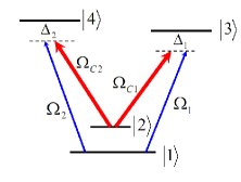
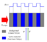
Figure 1: (Color online) (a) The energy-level structure (the double-$\Lambda$ scheme) of the active dopants (Pr³⁺). (b) The periodic distribution of the dopants (filling blue regions) against the background (gray regions). The dopant density is represented by function $R(x)$

The periodic modulation of the dopant concentration, i.e., the structure function $R(x)$, which represents the density of the implanted ions in Fig. 1(b), turns the uniform medium into a virtual PhC LYY1 -Jianxiong , so called because its properties are controlled by the pump fields, rather than by a permanent material structure (other well-known examples of virtual structures are lattices optically induced in photorefractive crystals Moti ). The density-modulation pattern induces an effective periodic linear potential, along with a spatially periodic modulation of all local optical parameters, including the strength of the linear interconversion and coefficients of the self-phase modulation (SPM). The virtual PhC of this type may be naturally called an inverted one, in comparison with ordinary (material) PhCs built in self-focusing media: While the ordinary PhC structures feature effective linear and nonlinear potentials with coinciding local minima, in the present setting minima of the local potential coincide with maxima of its nonlinear counterpart, and vice versa. i.e., the nonlinear potential is inverted with respect to the linear one LYY1 -LYY3 . Similar models with competing effective linear and nonlinear potentials were introduced, in a different context, in Ref. Kar12 . In fact, this setting may be considered as a variety of the general concept of nonlinear lattices and mixed linear-nonlinear ones NL .

The studies of the single-component model of the inverted virtual PhC with the Kerr and saturable nonlinearities, reported in Refs. LYY1 and LYY2 , respectively, have revealed that the stable location of the solitons in such systems is controlled by the total power, with the low- and high-power solitons tending to be pinned by minima of the linear and nonlinear potentials, respectively. Transitions between the different positions of the solitons were identified as supercritical SBBs.

The major objective of this work is to study two-component solitons, supported by the EIT scheme, in the inverted crystals, the main point being the SBBs of the solitons. In Sec. II, we derive the model by means of the semi-classical consideration of the interaction of the electromagnetic fields with atoms. Then, we focus on effects of the periodically modulated linear coupling between the two components, which is the main novel element of the model. In Sec. III, we consider the competition of the linear coupling and SPM nonlinearity. We concentrate on the SBB specific to the two-component system, and do not dwell on the above-mentioned breaking of the spatial symmetry of the solitons, which can be adequately studied in the single-component system LYY2 ; LYY3 . A systematic numerical analysis demonstrates a transition of the subcritical SBB into a supercritical one with the increase of the soliton’s total power, and a concomitant shrinkage of the soliton. In Sec. IV, analytical results are presented for an allied model of a dual-core fused fused spatial coupler, with the tightly concentrated linear coupling represented by the delta-function (in fact, the same system, but with a periodic array of coupled sites, and a periodic modulation of the refractive index and Kerr coefficient, may also represent the model of the virtual PhC considered in Sec. II). In that model, the SBB of two-component solitons can be studied in an exact analytical form. The paper is concluded by Sec. V.

II The model of the inverted nonlinear photonic crystal

The atomic Hamiltonian corresponding to the configuration shown in Fig. 1 is

$$H = \hbar[\delta|2\rangle\langle 2|+\Delta_{1}|3\rangle\langle 3|+\Delta_{2}|4\rangle\langle 4|]$$ (1)

$$-\hbar[\Omega_{1}|3\rangle\langle 1|+\Omega_{2}|4\rangle\langle 1|+\Omega_{C1}|3\rangle\langle 2|+\Omega_{C2}|4\rangle\langle 2|+\mathrm{H.c.}],$$

where fields $\Omega$ and detunings $\Delta_{1,2}$ are defined as per the figure, $\mathrm{H.c.}$stands for the Hermitian-conjugate contribution, and the two-photon detuning, $\delta$, is set to be zero. Under physically realistic conditions, spontaneous decay of the states included into the scheme may be neglected. Further, if the dopant atoms are initially kept in the ground state, steady-state solutions for density-matrix elements, $\rho_{31}$ and $\rho_{41}$, which are activated by the two soliton-forming probes, can be written as follows:

$$\rho_{31}=-{\frac{\Delta_{2}}{\Delta_{1}}}{\frac{|\Omega_{1}|^{2}}{\Omega_{C}^{2}}}\Omega_{1}-{\frac{|\Omega_{2}|^{2}}{\Omega_{C}^{2}}}\Omega_{1}+{\frac{|\Omega_{C2}|^{2}}{\Omega_{C}^{2}}}\Omega_{1}-{\frac{\Omega_{C1}\Omega_{C2}^{\ast}}{\Omega_{C}^{2}}}\Omega_{2},$$

$$\rho_{41}=-{\frac{\Delta_{1}}{\Delta_{2}}}{\frac{|\Omega_{2}|^{2}}{\Omega_{C}^{2}}}\Omega_{2}-{\frac{|\Omega_{1}|^{2}}{\Omega_{C}^{2}}}\Omega_{2}+{\frac{|\Omega_{C1}|^{2}}{\Omega_{C}^{2}}}\Omega_{2}-{\frac{\Omega_{C2}\Omega_{C1}^{\ast}}{\Omega_{C}^{2}}}\Omega_{2},$$ (2)

where $\Omega_{C}^{2}\equiv\Delta_{2}|\Omega_{C1}|^{2}+\Delta_{1}|\Omega_{C2}|^{2}$. The first (SPM) terms on the right-hand sides of Eqs. (2) originate from the self-enhanced Kerr effect XiaoM , the second and the third (XPM) terms represent the giant Kerr effect Schmidt , and the fourth terms represent the linear coupling between the soliton-forming beams, which originate from the EIT-induced frequency conversion HemmerHarrisHakuta .

The polarization experienced by the two probes in the medium are Scully

$$\mathscr{P}_{1}(x)=2N(x)\wp_{31}\rho_{31},$$

$$\mathscr{P}_{2}(x)=2N(x)\wp_{41}\rho_{41}.$$ (3)

Here,$\wp_{31}$ and $\wp_{41}$ (which are assumed real) are the matrix elements of the dipole transitions $|1\rangle\rightarrow|3\rangle$ and $|1\rangle\rightarrow|4\rangle$. A reasonable simplification of the model is attained by assuming that $\wp_{31}\approx\wp_{41}\equiv\wp$. The paraxial propagation equations for the slowly varying envelopes of the probe fields are

$$i\partial_{z}\Omega_{j}=-{\frac{1}{2k_{j}}}\partial_{xx}\Omega_{j}-{\frac{k_{j}\wp}{2\epsilon_{0}\hbar}}\mathscr{P}_{j}(x),[j=1,2].$$ (4)

Substituting Eq. (2) and Eq. (3) into Eqs. (4), one arrives at coupled nonlinear Schrödinger (NLS) equations,

$$i\partial_{z}\psi=-{\frac{1}{2}}\partial_{xx}\psi+R(x)\left(V_{1}\psi+\sigma_{1}|\psi|^{2}\psi+\kappa|\phi|^{2}\psi+C_{1}\phi\right),$$

$$i\partial_{z}\phi=-{\frac{1}{2}}\partial_{xx}\phi+R(x)\left(V_{2}\phi+\sigma_{2}|\phi|^{2}\phi+\kappa|\psi|^{2}\phi+C_{2}\psi\right).$$ (5)

where $\psi=\Omega_{1}/\gamma$, $\phi=\Omega_{2}/\gamma$, $R(x)={\wp^{2}}N(x)/\epsilon_{0}\hbar\gamma^{2}$, $V_{1}=-|\Omega_{C2}|^{2}/\Omega_{C}^{2}$, $V_{2}=-|\Omega_{C1}|^{2}/\Omega_{C}^{2}$, $\sigma_{1}=\Delta_{2}/\Delta_{1}\Omega_{C}^{2}$, $\sigma_{2}=\Delta_{1}/\Delta_{2}\Omega_{C}^{2}$, and $\kappa=1/\Omega_{C}^{2}$. If we let $\Omega_{C1}$ and $\Omega_{C2}$ be real, then coefficients $C_{1}=C_{2}\equiv C=\Omega_{C1}\Omega_{C2}/\Omega_{C}^{2}$ account for the EIT-induced linear mixing of the probe fields. The effective linear-coupling coefficient $CR(x)$ in Eq. (5), which is periodically modulated due to the distribution of the dopant density, makes the system different from various previously studied models of linearly-coupled systems Snyder -Amherst , Dror .

III Numerical results for the model of the photonic crystal

To focus on effects of the periodically modulated linear coupling competing with the SPM terms, we drop the XPM interaction in Eq. (5), and simplify Eqs. (5) to the following form:

$$i\partial_{z}\psi=-{\frac{1}{2}}\partial_{xx}\psi+V(x)\left(1-|\psi|^{2}\right)\psi-C(x)\phi,$$

$$i\partial_{z}\phi=-{\frac{1}{2}}\partial_{xx}\phi+V(x)\left(1-|\phi|^{2}\right)\phi-C(x)\psi.$$ (6)

These equations generalize those derived in Refs. LYY1 ; LYY2 for the inverted PhC with the $\pi$-shift between the periodic linear and nonlinear potentials, under the assumption that the depletion of the coupling fields, $\Omega_{C1}$ and $\Omega_{C2}$ [see Fig. 1(a)], may be neglected. In this work, we consider the density-distribution profile in Fig. 1(b) corresponding to $R(x)=\cos^{2}x$, i.e., $V(x)=V_{0}\cos^{2}x$, $C(x)=C_{0}\cos^{2}x$, the notation being fixed by scaling the modulation period to be $\pi$. Generic results are displayed below for amplitude $V_{0}=0.5$ of the nonlinearity modulation, while strength $C_{0}$ of the linear coupling is varied. As for the sign of $C_{0}$, it may be fixed to be positive, as $C_{0}<0$ can be transformed into $C_{0}>0$ by the change of $\phi\rightarrow-\phi$, while the sign of $\psi$ is not altered.

Stationary soliton solutions to Eqs. (6) were found in a numerical form by means of the imaginary-time propagation method Chiofalo , and their stability was subsequently tested by direct simulations of the perturbed evolution in real time. The solitons are characterized by the total power,

$$P\equiv P_{1}+P_{2}=\int_{-\infty}^{+\infty}\left[|\psi(x)|^{2}+|\phi(x)|^{2}\right]dx.$$ (7)

As expected, both symmetric and asymmetric soliton modes, in terms of the coupled components, were found, see Figs. 2 and 3. These examples display stable solitons, which are broad in comparison with the underlying modulation pattern at smaller values of $P$ [Fig. 2], and narrower modes, with the width comparable to the modulation period, at larger $P$ [Fig. 3].

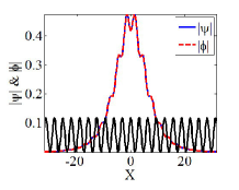
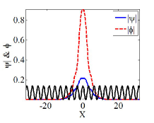
Figure 2: (Color online) Stationary profiles of the two components of stable symmetric (a) and asymmetric (b) solitons, both found for $P=4$, $C_{0}=0.078$. These solitons belong to the bifurcation diagram displayed in Fig. 4(a). In this figure and below, the black solid lines display the shape of the underlying modulation function, $R(x)$ [see Fig. 1(b)].

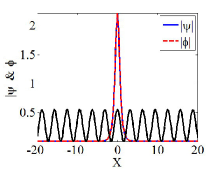
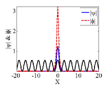
Figure 3: (Color online) Examples of stable symmetric (a) and asymmetric (b) solitons found for $P=10$ and $C_{0}=2$ (a) or $C=1.5$ (b). These solitons belong to the bifurcation diagram displayed in Fig. 4(d).

The numerical results are summarized in the form of bifurcation diagrams displayed in Fig. 4 at different fixed values of the total power, $P$. The bifurcations are driven by the decrease of the coupling coupling, $C_{0}$. Unstable branches of symmetric solitons, which should continue the stable ones in all the panels, and narrow intermediate branches of unstable asymmetric solitons in panel 4(a), are missing as the imaginary-time integration method does not converge to unstable solutions. The diagrams show the transition from the subcritical SBB to the supercritical bifurcation with the increase of $P$.

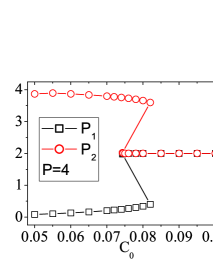
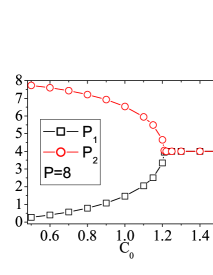
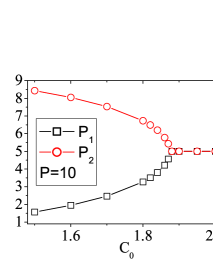
Figure 4: (Color online) The bifurcation diagrams for the two-component solitons with different fixed values of the total power, corresponding to the variation of strength $C_{0}$ of the linear coupling. Panels (a,b) and (c,d) correspond to the bifurcations of the sub- and super-critical types, respectively.

For broad solitons one may replace $R(x)=\cos^{2}x$ in Eqs. (6) by its mean value, $\left\langle\cos^{2}x\right\rangle=1/2$, which reduces the system to the one studied in earlier works Snyder , where the SBB is subcritical, in accordance with Fig. 4(a). The new situation is actually found here for narrow solitons, for which the SBB turns out to be supercritical.

It is instructive to compare these results with those found in a system where the linear and nonlinear potentials are the same as in Eqs. (6), but the linear coupling is made constant, by replacing $C_{0}\cos^{2}(x)\rightarrow C_{0}/2$:

$$i\partial_{z}\psi=-{\frac{1}{2}}\partial_{xx}\psi+V(x)\left(1-|\psi|^{2}\right)\psi-\frac{1}{2}{C_{0}}\phi,$$

$$i\partial_{z}\phi=-{\frac{1}{2}}\partial_{xx}\phi+V(x)\left(1-|\phi|^{2}\right)\phi-\frac{1}{2}{C_{0}}\psi.$$ (8)

Figure 5 demonstrates that the modified system does not give rise to the transition of the subcritical SBB into the supercritical type, even in the case when $P$ is large and the solitons are narrow. Thus, the periodic modulation of the linear coupling is essential for this transition.

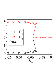
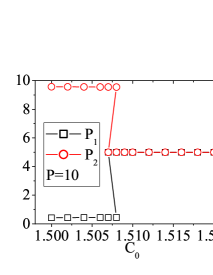
Figure 5: (Color online) The bifurcation diagrams for the two-component solitons produced by modified system (8).

IV Analytical results for the fused coupler

Numerical finding presented in the previous section suggest that the spatial modulation of the linear coupling is a crucial factor which determines the kind of the phase transition (SBB) in the system, and the possible change of the kind. In this section, we aim to illustrate the genericity of this rule by means of exact analytical results, obtained in an allied system which describes a fused dual-core nonlinear planar waveguide fused , with the linear coupling tightly concentrated at $x=0$:

$$i\partial_{z}\psi = -\frac{1}{2}\partial_{xx}\psi-\left|\psi\right|^{2}\psi-2\delta(x)\phi,$$

$$i\partial_{z}\phi = -\frac{1}{2}\partial_{xx}\phi-\left|\phi\right|^{2}\phi-2\delta(x)\psi,$$ (9)

where $\delta(x)$ is the delta-function. This system is a limit case of Eqs. (6), with $C(x)=2\delta(x)$ and $V(x)\equiv 1$ (in that case, the constant linear potential is trivial in the present case and may be dropped). Coefficients in the system can be fixed as in Eqs. (9) by means of an obvious rescaling. It is relevant to mention that symmetric and asymmetric solitons in a discrete version of this system were recently studied in Ref. Belgrade , but the discrete system does not admit exact solutions. In fact, the underlying system of Eqs. (6) may also be realized in terms of the dual-core spatial coupler, with periodically modulated strength of the coupling, refractive index, and Kerr coefficient.

Stationary solutions to Eqs. (9) are sought for as $\left\{\psi,\phi\right\}=\exp\left(ikz\right)\left\{u(x),v(x)\right\},$ with real functions $u(x)$ and $v(x)$ satisfying equations

$$ku = \frac{1}{2}u^{\prime\prime}+u^{3}+2\delta(x)v,$$

$$kv = \frac{1}{2}v^{\prime\prime}+v^{3}+2\delta(x)u.$$ (10)

Obviously, solutions to Eqs. (10) are subject to the following boundary conditions, produced by the integration in an infinitesimal vicinity of $x=0$:

$$u^{\prime}\left(x=+0\right)-u^{\prime}\left(x=-0\right) = -4v\left(x=0\right),~{}$$

$$v^{\prime}\left(x=+0\right)-v^{\prime}\left(x=-0\right) = -4u\left(x=0\right).$$ (11)

Exact soliton solutions to Eqs. (10) are looked for as

$$\left\{u(x),v(x)\right\}=\sqrt{2k}\mathrm{sech}\left(\sqrt{2k}\left(|x|+\left\{\xi,\eta\right\}\right)\right)$$ (12)

with $\xi,\eta>0$. Symmetric and asymmetric solutions correspond to $\xi=\eta$ and $\xi\neq\eta$, respectively (the present model does not admit antisymmetric solutions). Total power (7) of solutions (12) is

$$P=2\sqrt{2k}\left[2-\tanh\left(\sqrt{2k}\xi\right)-\tanh\left(\sqrt{2k}\eta\right)\right].$$ (13)

The substitution of expressions (12) into Eqs. (11) yields the following equations which determine positive constants $\xi$ and $\eta$:

$$\sqrt{\frac{k}{2}}\sinh\left(\sqrt{2k}\left\{\xi,\eta\right\}\right)\mathrm{sech}^{2}\left(\sqrt{2k}\left\{\xi,\eta\right\}\right)=\mathrm{sech}\left(\sqrt{2k}\left\{\eta,\xi\right\}\right).$$ (14)

Using notation $t_{1,2}\equiv\tanh\left(\sqrt{2k}\left\{\xi,\eta\right\}\right)$, Eqs. (14) can be transformed into the following form:

$$\left(t_{1}-t_{2}\right)\left(t_{1}^{2}+t_{2}^{2}+t_{1}t_{2}-1\right) = 0,$$ (15)

$$t_{1}t_{2} = 2/k,$$ (16)

where physical solutions are constrained to $0<t_{1,2}<1$. Equation (15) gives two solutions: $t_{1}=t_{2}$, which corresponds to symmetric solitons, and the other solution, which corresponds to asymmetric ones:

$$t_{1}^{2}+t_{2}^{2}+t_{1}t_{2}=1.$$ (17)

As it follows from Eq. (16), the symmetric solutions have

$$\tanh\left(\sqrt{2k}\left\{\xi,\eta\right\}\right)=\sqrt{2/k},$$ (18)

hence they exist only for $k>2$, the total power (13) of the symmetric soliton being

$$P_{\mathrm{symm}}=4\sqrt{2}\left(\sqrt{k}-\sqrt{2}\right).$$ (19)

The phase transition (SBB) occurs when the symmetric solution, $t_{1}=t_{2}=\sqrt{2/k}$, is simultaneously a solution to Eq. (17), which yields

$$k=6,~{}\tanh\left(2\sqrt{3}\left\{\xi,\eta\right\}\right)=\frac{1}{\sqrt{3}},~{}P_{\mathrm{symm}}=\frac{16}{\sqrt{3}}.$$ (20)

The solution for the asymmetric solitons, following from Eqs. (17) and (16), is

$$\tanh^{2}\left(\sqrt{2k}\left\{\xi,\eta\right\}\right)=\frac{k-2\pm\sqrt{k^{2}-4k-12}}{2k},$$ (21)

which exists exactly at $k>6$, cf. Eq. (20). Further, the total power (13) of the asymmetric soliton is

$$P_{\mathrm{asymm}}=2\left[2\sqrt{2k}-\left(\sqrt{k-2+\sqrt{k^{2}-4k-12}}+\sqrt{k-2-\sqrt{k^{2}-4k-12}}\right)\right],$$ (22)

and the relative asymmetry of the soliton is

$$\Theta\equiv\frac{P_{1}-P_{2}}{P_{2}+P_{2}}=$$

$$\pm\frac{\sqrt{k-2+\sqrt{k^{2}-4k-12}}-\sqrt{k-2-\sqrt{k^{2}-4k-12}}}{2\sqrt{2k}-\left(\sqrt{k-2+\sqrt{k^{2}-4k-12}}+\sqrt{k-2-\sqrt{k^{2}-4k-12}}\right)}.$$ (23)

Figure 6 plots asymmetry $\Theta$ versus $P_{\text{asymm}}$, as obtained from Eqs. (23) and (22). The figure confirms that the SBB is indeed of the supercritical type when the linear coupling is spatially localized.

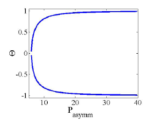
Figure 6: (Color online) Asymmetry $\Theta$ versus total power $P_{\text{asymm}}$, in the solvable model based on Eqs. (9).

The model based on Eqs. (9) is solvable too in the case of the self-defocusing nonlinearity, corresponding to the opposite signs in front of the cubic terms. However, in that case the model admits solely symmetric solutions, in the form of $u(x)=v(x)=\sqrt{2k}/\mathrm{\sinh}\left(\sqrt{2k}\left(|x|+\xi\right)\right)$, with $\xi$ determined by equation $\tanh\left(\sqrt{2k}\xi\right)=\sqrt{k/2}$, which has solutions for $k<2$, cf. Eqs. (12) and (18).

V Conclusions

The objective of this work is to study the SBBs (symmetry-breaking bifurcations) of solitons in two-component systems which, unlike previously studied models, include the spatial modulation of the linear-coupling strength. To this end, two photonic models were considered, namely, the inverted virtual PhC (photonic crystal), and the fused dual-core spatial coupler. The former system is built as the periodic distribution of the density of dopant atoms, activated by the EIT, which induces the linear mixing between the two probe fields. The periodic density modulation makes all parameters of the medium periodic functions of the coordinate. Disregarding the XPM terms, we have found that the type of the SBB changes from sub- to supercritical with the increase of the total power of the probe beams. In the model of the fused dual-core coupler, the solutions for the two-component solitons were obtained in the exact form, the corresponding SBB being supercritical.

The work can be naturally extended in other directions, including the interplay with the spatial symmetry breaking, and the consideration of higher-order solitons. A challenging possibility is to develop a two-dimensional generalization of the system.

- (1) A. W. Snyder, D. J. Mitchell, L. Poladian, D. R. Rowland, and Y. Chen, J. Opt. Soc. Am. B, 8, 2101 (1991); S. Trillo, S. Wabnitz, E. M. Wright, and G. I. Stegeman, Opt. Lett. 13, 672 (1988); E. M. Wright, G. I. Stegeman, S. Wabnitz, Phys. Rev. A 40, 4455 (1989); C. Paré and M. Fłorjańczyk, ibid. 41, 6287 (1990); A. I. Maimistov, Kvant. Elektron. 18, 758 [Sov. J. Quantum Electron. 21, 687 (1991)]; M. Romagnoli, S. Trillo, and S. Wabnitz, Opt. Quantum Electron. 24, S1237 (1992); N. Akhmediev and A. Ankiewicz, Phys. Rev. Lett. 70, 239 (1993); P. L. Chu, B. A. Malomed, and G. D. Peng, Opt. Lett. 18, 328 (1993); Y. S. Kivshar and M. L. Quiroga-Teixeiro, ibid. 18, 980 (1993); K. S. Chiang, Opt. Lett. 20, 997 (1995); A. Mostofi, B. A. Malomed, and P. L. Chu, Opt. Commun. 137, 244 (1997); ibid. 145, 274 (1998).
- (2) A. Gubeskys and B. A. Malomed, Phys. Rev. A 75, 063602 (2007); 76, 043623 (2007); M. Matuszewski, B. A. Malomed, and M. Trippenbach, Phys. Rev. A 75, 063621 (2007); L. Salasnich, B. A. Malomed, and F. Toigo, ibid. 81, 045603 (2010).
- (3) M. Trippenbach, E. Infeld, J. Gocalek, M. Matuszewski, M. Oberthaler, and B. A. Malomed, Phys. Rev. A 78, 013603 (2008).
- (4) Y. S. Kivshar and G. P. Agrawal, Optical Solitons: From Fibers to Photonic Crystals (Academic Press: San Diego).
- (5) N. V. Hung, M. Trippenbach, and B. A. Malomed, Phys. Rev. A 84, 053618 (2011).
- (6) G. Herring, P. G. Kevrekidis, B. A. Malomed, R. Carretero-González, and D. J. Frantzeskakis, Phys. Rev. E 76, 066606 (2007).
- (7) Lj. Hadžievski, G. Gligorić, A. Maluckov, and B. A. Malomed, Phys. Rev. A 82, 033806 (2010).
- (8) M. V. Tratnik and J. E. Sipe, Phys. Rev. A 38, 2011 (1988); S. Trillo, S. Wabnitz, E. M. Wright and G. I. Stegeman, Opt. Commun. 70, 166 (1989); B. A. Malomed, Phys. Rev. E 50, 1565 (1994).
- (9) H. Sakaguchi and B. A. Malomed, Phys. Rev. E 83, 036608 (2011); N. Dror, B. A. Malomed, and J. Zeng, ibid. 84, 046602 (2011).
- (10) R. J. Ballagh, K. Burnett, and T. F. Scott, Phys. Rev. Lett. 78, 1607 (1997); A. Kuklov, N. Prokof’ev, and B. Svistunov, Phys. Rev. A 69, 025601 (2004); J. Williams, R. Walser, J. Cooper, E. Cornell, and M. Holland, ibid. 59, R31 (1999); P. Öhberg and S. Stenholm, ibid. 59, 3890 (1999); D. T. Son and M. A. Stephanov, ibid. 65, 063621 (2002); S. D. Jenkins and T. A. B. Kennedy, ibid. Phys. Rev. A 68 053607 (2003); Q.-H. Park and J. H. Eberly, ibid. A 70, 021602(R) (2004); I. M. Merhasin, B. A. Malomed, and R. Driben, J. Phys. B: At. Mol. Opt. Phys. 38, 877 (2005); S. K. Adhikari, and B. A. Malomed, Phys. Rev. A 79, 015602 (2009).
- (11) V. A. Brazhnyi and B. A. Malomed, Phys. Rev. A. 83, 053844 (2011).
- (12) Y. Wu, and L. Deng, Phys. Rev. Lett. 93, 143904 (2004); G. Huang, L. Deng, and M. G. Payne, Phys. Rev. E 72 016617 (2005); J. Wang, C. Hang, and G. Huang, Phys. Lett. A 366 528 (2007); G. Huang, K. Jiang, M. G. Payne, and L. Deng, Phys. Rev. Lett. 73 056606(2006); T. Hong, Phys. Rev. Lett. 90 183901(2003); C. Hang, G. Huang, and L. Deng, Phys. Rev. E 74 046601(2006).
- (13) H. Wang,D. Goorskey, and M. Xiao, Phys. Rev. Lett. 87, 073601 (2001).
- (14) H. Schmidt and A. Imamoǧlu, Opt. Lett. 21, 1936 (1996).
- (15) S. E. Harris, J. E. Field, and A. Imamoǧlu, Phys. Rev. Lett. 64, 1107 (1990).
- (16) M. Fleischhauer, A. Imamoglu, J. P. Marangos, Rev. Mod. Phys. 77, 633 (2005).
- (17) P. R. Hemmer, D. P. Katz, J. Donoghue, M. Cronin-Golomb, M. S. Shariar, and P. Kumar, Opt. Lett. 20, 769 (1995); S. E. Harris, and A. V. Sokolov, Phys. Rev. A. 55, R4019 (1997); K. Hakuta, M. Suzuki, M. Katsuragawa, and J. Z. Li, Phys. Rev. Lett. 79, 209 (1997).
- (18) E. A. Korsunsky and D. V. Kosachiov, Phys. Rev. A. 60, 4996 (1999).
- (19) M. Feng, Y. Liu, Y. Li, X. Xie, and J. Zhou, Opt. Exp. 19, 7222 (2011); J. Li, B. Liang, Y. Liu, P. Zhang, J. Zhou, S. O. Klimonsky, A. S. Slesarev, Y. D. Tretyakov, L. O’Faolain, and T. F. Krauss, Adv. Mater. 22, 1 (2010).
- (20) Y. Li, B. A. Malomed, M. Feng, and J. Zhou, Phys. Rev. A. 82, 063823 (2010).
- (21) Y. Li, B. A. Malomed, M. Feng, and J. Zhou, Phys. Rev. A. 83, 053832(2011).
- (22) Y. Li, B. A. Malomed, J. Wu, W. Pang, S. Wang, and J. Zhou, Phys. Rev. A 84, 043839 (2011).
- (23) J. Wu, M. Feng, W. Pang, S. Fu, and Y. Li, J. Nonlin. Opt. Phys. 20, 193 (2011).
- (24) N. K. Efremidis, S. Sears, D. N. Christodoulides, J. W. Fleischer, and M. Segev, Phys. Rev. E 66, 046602 (2002); N. K. Efremidis, J. Hudock, D. N. Christodoulides, O. Cohen, and M. Segev, Phys. Rev. Lett. 91, 213905 (2003); J. W. Fleischer, G. Bartal, O. Cohen, T. Schwartz, O. Manela, B. Freedman, M. Segev, H. Buljan, and N. K. Efremidis, Opt. Express 13, 1780 (2005).
- (25) Y. V. Kartashov, V. A. Vysloukh, and L. Torner, Opt. Lett., 33, 1747 (2008); ibid. 33, 2173 (2008); T. Mayteevarunyoo and B. A. Malomed, J. Opt. Soc. Am. B 25, 1854 (2008).
- (26) Y. V. Kartashov, B. A. Malomed, and L. Torner, Rev. Mod. Phys. 83, 247 (2011).
- (27) L. Eldada, Opt. Engineering 40, 1165 (2001).
- (28) M. O. Scully and M. S. Zubairy, Quantum Optics (Cambridge University, Cambridge, England, 1997).
- (29) M. L. Chiofalo, S. Succi, and M. P. Tosi, Phys. Rev. E, 62, 7438 (2000). J. Yang, and T. I. Lakoba, Stud. Appl. Math., 120, 265 (2008). J. Yang, and T. I. Lakoba, Stud. Appl. Math., 118, 153 (2007).