Clustering of star-forming galaxies detected in mid-infrared with the Spitzer wide-area survey

Abstract

We discuss the clustering properties of galaxies with signs of ongoing star formation detected by the Spitzer Space Telescope at $24\,\mu\rm m$ band in the SWIRE Lockman Hole field. The sample of mid-IR-selected galaxies includes $\sim 20000$ objects detected above a flux threshold of $S_{24\,\mu\rm m}=310\,\mu$Jy. We adopt optical/near-IR color selection criteria to split the sample into the lower-redshift and higher-redshift galaxy populations. We measure the angular correlation function on scales of $\theta=0.01-3.5$ deg, from which, using the Limber inversion along with the redshift distribution established for similarly selected source populations in the GOODS fields (Rodighiero et al., 2010), we obtain comoving correlation lengths of $r_{0}=4.98\pm 0.28\,h^{-1}\,$Mpc and $r_{0}=8.04\pm 0.69\,h^{-1}\,$Mpc for the low-$z$ ($z_{\rm mean}=0.7$) and high-$z$ ($z_{\rm mean}=1.7$) subsamples, respectively. Comparing these measurements with the correlation functions of dark matter halos identified in the Bolshoi cosmological simulation (Klypin et al., 2011), we find that the high-redshift objects reside in progressively more massive halos reaching $M_{\rm tot}\gtrsim 3\times 10^{12}\,h^{-1}\,M_{\odot}$, compared to $M_{\rm tot}\gtrsim 7\times 10^{11}\,h^{-1}\,M_{\odot}$ for the low-redshift population. Approximate estimates of the IR luminosities based on the catalogs of $24\,\mu\rm m$ sources in the GOODS fields show that our high-$z$ subsample represents a population of “distant ULIRGs” with $L_{\rm IR}>10^{12}L_{\odot}$, while the low-$z$ subsample mainly consists of “LIRGs”, $L_{\rm IR}\sim 10^{11}L_{\odot}$. The comparison of number density of the $24\,\mu\rm m$ selected galaxies and of dark matter halos with derived minimum mass $M_{\rm tot}$ shows that only 20% of such halos may host star-forming galaxies.

1. Introduction

The cosmic infrared background (CIB; Puget et al., 1996; Hauser et al., 1998) accounts for approximately half of the total extragalactic background energy integrated over cosmic time and wavelengths (e.g., Dole et al., 2006; Hauser & Dwek, 2001). The CIB emission is mainly contributed by star-forming galaxies where optical–UV light from young stellar populations is absorbed by dust and re-emitted at longer wavelengths. The IR-energy output per unit volume must strongly increase with redshift to account for the total measured CIB (Hauser & Dwek, 2001; Lagache et al., 2005). Indeed, observations with the Infrared Space Observatory (ISO; Genzel & Cesarsky, 2000) and the Spitzer Space Telescope (Werner et al., 2004) revealed large number of distant mid- and far-infrared sources (Chary & Elbaz, 2001; Elbaz et al., 2002; Le Floc’h et al., 2005). According to the current consensus from both theoretical and observational studies, major developments in the evolution of galaxies in the universe happened at high redshifts, $z>1$ (for references and details, see Franceschini et al., 2010), with the peak of star formation and nuclear activity occurring at $z\sim 2$ (e.g., Madau et al., 1996; Hopkins, 2004; Silverman et al., 2005; Bouwens et al., 2011). A large fraction of energy emitted during these active phases of galaxy evolution is hidden by dust and can be detected only through mid- and far-IR observations. Therefore, studying the distant universe in the infrared provides valuable information on the history of assembly of present-day massive galaxies (e.g., Soifer et al., 2008; Le Floc’h et al., 2009; Santini et al., 2009; Franceschini et al., 2010).

In this work, we use observations of star-forming galaxies made by the Spitzer Space Telescope at $24\,\mu\rm m$. The Spitzer $24\,\mu\rm m$ surveys have revolutionized studies of “distant ULIRGs” — ultraluminous infrared galaxies. These objects are dusty star-forming galaxies with infrared luminosity $L_{\rm IR}>10^{12}L_{\odot}$ (e.g., Rigby et al., 2004; Yan et al., 2005; Daddi et al., 2007; Fiolet et al., 2010; Fadda et al., 2010). While the average spectral energy distribution of high-$z$ sources is consistent with that of present-day ULIRGs, the nature and the cosmological environment hosting them must still be clarified (see Huang et al., 2009, for details and references). Various photometric techniques are applied to identify high-redshift objects among the thousands detected by wide-field Spitzer surveys, e.g., Yan et al. (2005), Magliocchetti et al. (2007), Farrah et al. (2008), Lonsdale et al. (2009), Fiolet et al. (2009), Huang et al. (2009), and Dey et al. (2008). All these selected objects represent sub-populations of ULIRGs with observational characteristics partly overlapping those of star-forming galaxies detected in optical and submillimeter (see recent papers by Huang et al., 2009; Fiolet et al., 2009). The nature of these populations has been a subject of intensive work based on modeling of their physical properties such as spectral energy distribution (SED), star formation rate, stellar and halo masses, etc. (e.g., Granato et al., 2004; Davé et al., 2010; Narayanan et al., 2010; Lacey et al., 2010). A significant new observational input for such studies can be provided by measurements of the clustering amplitude, which is a unique tool for determination of the halo masses of high-redshift galaxies. The goal of this paper is to present clustering and halo occupation analysis of $24\,\mu\rm m$ detected galaxies from one of the largest Spitzer extragalactic survey.

First studies on clustering of $24\,\mu\rm m$ galaxies were made either in small fields with low statistics, e.g.,  Gilli et al. (2007) and Magliocchetti et al. (2008), or applying additional selection criteria as in Farrah et al. (2006) and Brodwin et al. (2008). Here we improve on these first measurements by using a large sample of $\sim 20,000$ galaxies detected in the Lockman Hole field, $\sim 8$ deg², and uniformly selected only by their $24\,\mu\rm m$ flux, $S_{24\,\mu\rm m}>310\,\mu$Jy. Our data reduction procedures are presented in Section 2. The clustering strength measurements of $24\,\mu\rm m$ selected galaxies and inferred properties of their dark matter (DM) halos are discussed in Sections 3 and 4. Comparison with previously published results is presented in Section 5, and our conclusions appear in Section 6.

Throughout the paper, all cosmology-dependent quantities are computed assuming a spatially flat model with parameters $\Omega_{\rm M}=0.268$ and $\Omega_{\rm\Lambda}=0.732$ (best-fit $\Lambda$CDM parameters obtained from the combination of CMB, supernovae, baryon acoustic oscillations, and galaxy cluster data, see Vikhlinin et al., 2009). All distances are comoving and given with explicit h-scaling, where the Hubble constant is $H_{0}=100\,h^{-1}\,\rm{km\,s^{-1}\,Mpc^{-1}}$. The parameter uncertainties are quoted at a confidence level of 68%. IR luminosities were computed using $H_{0}=70\,\rm{km\,s^{-1}\,Mpc^{-1}}$ (see Rodighiero et al., 2010,  for details).

2. The data sample

For reliable clustering measurements one needs a statistically complete, large, and homogeneous sample of sources selected over a large area of the sky to probe the correlation signal on a wide range of scales. The Spitzer Wide-area InfraRed Extragalactic Survey (SWIRE, Lonsdale et al., 2003) is highly suitable for this purpose, as was demonstrated in several papers (Waddington et al., 2007; de la Torre et al., 2007; Farrah et al., 2006). It is the largest survey carried out with the Spitzer Space Telescope, covering $\sim 49\,\rm{deg}^{2}$ in six separate fields in the Northern and Southern sky. Each field was imaged in the seven near-to-far infrared bands: InfraRed Array Camera (IRAC) 3.6, 4.5, 5.8, 8.0 $\,\mu\rm m$ (Fazio et al., 2004) and Multiband Imaging Photometer for Spitzer (MIPS) 24, 70, and 160 $\,\mu\rm m$ bands (Rieke et al., 2004). In addition to the infrared observations, every SWIRE field has high-quality ancillary data.

Following the goal of our work to estimate the correlation function of star-forming galaxies detected in the MIPS $24\,\,\mu\rm m$ band, we first selected a sample of bright sources, $S_{24\,\mu\rm m}>400\,\mu$Jy, from the SWIRE ELAIS-S1 catalog (M. Vaccari et al., in preparation). However, our estimated angular correlation function, $w(\theta)$, showed an unexpected lack of clustering signal at scales $\theta<36^{\prime\prime}$. There were suggestions in the literature (e.g., Gilli et al., 2007) that because of the poor angular resolution of the MIPS instrument ($\sim 6^{\prime\prime}$ FWHM), there could be difficulties in determining $w(\theta)$ for faint sources due to blending. However, the deficit of close pairs in the sample of bright sources remained unexplained. This problem has no bearing on our main results presented below but obviously its origin needs to be understood. To this end, we carried out a comparison of the angular correlation function of the $24\,\,\mu\rm m$ sources selected from the four largest SWIRE fields (Lockman Hole, ELAIS-N1, ELAIS-N2, and CDFS) using two releases of the SWIRE team catalogs (versions 2005 and 2010), and an additional source catalog based on the wavelet decomposition algorithm (Section 2.1). This comparison is reported in the Appendix. Our clustering results for 24  $\mu\rm m$ sources presented below are based on the best available catalog in the Lockman Hole field.

2.1. Wavelet-based Detection of 24 $\mu\rm m$ Sources

Due to the reasons outlined in the Appendix, we perform clustering analysis of 24 $\mu\rm m$ sources extracted from the publicly available MIPS images using the wavelet decomposition source detection algorithm (wvdecomp, see Vikhlinin et al., 1998). This algorithm at $S_{24\,\mu\rm m}\gtrsim 300\,\mu$Jy performs nearly identically to the detection method used in the Final SWIRE Data Release (J. A. Surace et al., in preparation) in terms of the $\log N-\log S$ distribution of detected sources and their angular correlation function at large scales. The only noticeable difference is in the treatment of very crowded regions and zones in the immediate vicinity of the bright sources (see the Appendix). These differences have no effect on our clustering results presented in Section 3 and 4 below.

wvdecomp was designed to efficiently detect both point-like and slightly extended sources in the crowded fields. Originally, the wavelet decomposition program was intended for Poisson-noise-limited X-ray images, where it generally outperforms its rivals (Revnivtsev et al., 2007), but it was found that with a suitable choice of parameters, it produces good results also for the 24  $\mu\rm m$ MIPS images.

First, we re-bin the archival MIPS images to $2.4^{\prime\prime}$ pixels (by a factor of two with respect to an original pixel size of $1.2^{\prime\prime}$) to reduce the cross-correlation of noise in the adjacent pixels while still maintaining the adequate sampling of the PSF. We then convolve the image with the ${\rm scale}=2$ wavelet filter, corresponding to an effective kernel width of $\approx 5^{\prime\prime}-6^{\prime\prime}$, matching the size of the MIPS 24  $\mu\rm m$ point sources. The rms of variations in this convolved image, excluding the regions around bright sources using $\sigma$-clipping, is the approximation of effective noise at the scale we are most interested in. This noise level is supplied to the wvdecomp program (its internal noise determination algorithm is best suitable for the case Poisson statistics and thus not applicable for MIPS images). wvdecomp starts with the smallest scales and iteratively detects and removes detected structures from the input image, while adding them to the resulting “clean” image. When the process is finished at the given scale, it proceeds to the next at which the size of the wavelet kernel is increased by a factor of two. In our case, the detection algorithm works on the scales corresponding to structure sizes (FWHM) of $\approx 2.4^{\prime\prime}$, $5^{\prime\prime}$, and $10^{\prime\prime}$, bracketing the range of sizes for the MIPS point sources. Detection threshold is set at $4.5\sigma$, at which we expect $\sim 100$ false detections in the Lockman Hole area.

The main output of the wavelet decomposition algorithm is a list of source locations detected above a predefined SNR threshold, and a map which allows one to split the original image into “empty” regions and those with significant emission “belonging” to a particular source. The source fluxes were then measured using aperture photometry. In choosing the aperture size, the tradeoff is between our desire to include as much of the source flux as possible into the aperture size, and the fact that for wide apertures, the flux measurements are increasingly affected by the larger-scale background fluctuations and by source confusion. Several tests have shown that the best results are achieved for an aperture size of $4^{\prime\prime}$, encompassing approximately 50% of the PSF power, and corresponding to the bright core of the MIPS PSF. These aperture fluxes were then converted into total flux using the PSF model calibrated with images of the bright stars in the same field. Using this method, the 24  $\mu\rm m$ sources were extracted from the MIPS map of the Lockman Hole field.

2.2. The Lockman Hole Source Sample

The Lockman Hole is the largest of the SWIRE fields. In addition to deeper MIPS observations (the limiting flux is $S_{24\,\mu\rm m}=310\,\mu$Jy, compared, e.g., to $S_{24\,\mu\rm m}=400\,\mu$Jy in the ELAIS-S1 field, see Appendix B for details), it has deep and uniform data in many other bands. In particular, we used the data from the Two Micron All Sky Survey (2MASS) survey for the star-mask construction (see Section 2.2.1), and the optical observations carried out with INT-WFC and KPNO MOSAIC1 (González-Solares et al., 2011) to photometrically separate the 24  $\mu\rm m$-selected objects into the low- and high-redshift subsamples (Section 2.2.2).

We cross-correlated our sample of 24  $\mu\rm m$ sources with the multi-band IRAC-based catalog (limiting fluxes of $S_{3.6\,\mu\rm m}\simeq 7\,\mu$Jy and $S_{4.5\,\mu\rm m}\simeq 11\,\mu$Jy, M. Vaccari et al., in preparation) using a matching radius of $3.2^{\prime\prime}$. We then applied the following flux cuts: $310<S_{24\,\mu\rm m}<2500\,\mu$Jy and $S_{3.6\,\mu\rm m}<1000\,\mu$Jy, and $S_{4.5\,\mu\rm m}<1000\,\mu$Jy. $S_{24\,\mu\rm m}=310\,\mu$Jy is the flux at which the catalog is complete and the fluxes are measured reliably and accurately. The bright flux cuts are applied in order to conservatively discard obviously extended and/or saturated sources whose astrometry may be poor and whose flux estimates may be affected by saturation. Only $1.7\%$ of sources with $S_{24\,\mu\rm m}>310\,\mu$Jy had no IRAC-couterparts. A small fraction of them are Galactic stars, $\sim 0.3\%$ are expected due to false detections for our choice of wvdecomp detection thresholds, the nature of the rest is unclear. In any case, their number is too small to affect our clustering measurements.

2.2.1 Elimination of Stars and the Region Mask

Galactic stars contaminate our clustering analysis of extragalactic sources and should be removed. To this end, we followed the procedures of  Shupe et al. (2008) and  Waddington et al. (2007) in which the foreground stars were identified using the 2MASS Point Source Catalog (Skrutskie et al., 2006). The derived $24\,\mu\rm m$-IRAC catalog was cross correlated with the 2MASS survey using a matching radius of $2.5^{\prime\prime}$. Shupe et al. (2008) proposed that nearly all of the $24\,\,\mu\rm m$-emitting sources with color $K_{s}-[24]<2.0$ (Vega, mag) are Galactic stars (see their Figure  2). We applied this criterion to our catalog and eliminated such sources.

In addition to directly polluting the extragalactic sample, bright Galactic stars may affect our clustering measurements indirectly, by obscuring the background galaxies or affecting the fluxes of the fainter galaxies near the same line of sight. Therefore, we need to completely exclude from the analysis the sky regions affected by the presence of bright foreground stars. Following Waddington et al. (2007) this was achieved by masking out the circular regions around sources with $K_{s}<12$ (Vega, mag) from the cross-correlated $24\,\mu\rm m$-IRAC-2MASS catalog; the exclusion radius was determined as $\log(R^{\prime\prime})=3.1-0.16\,K_{s}$, which is the distance at which the stellar PSF merges into the background (Waddington et al., 2007).

A close examination of the $24\,\mu\rm m$ source catalog shows that there are spurious detections around very bright $24\,\mu\rm m$ sources (most of which correspond to Galactic stars or low-$z$ galaxies). Therefore, we decided to mask out those regions as well. The exclusion radius was set to be $20^{\prime\prime}-80^{\prime\prime}$, depending on the source flux.

As we will discuss in the next section, Section 2.2.2, we use the INT/WFC optical data to divide our sample photometrically into the low- and high-redshift subsamples. Unfortunately, the INT/WFC observations are insufficiently deep in some subsections of the MIPS Lockman Hole image, and we had to mask out those regions also. To identify the regions of insufficient INT/WFC depth, we examined the distribution of optical counterparts for $3.6\,\,\mu\rm m$ IRAC sources at various $i$-band magnitude cuts. We found that the depth is at least $i=22.8$ throughout the field, except for the regions masked out as rectangles in Figure 1. At fainter magnitudes, the WFC coverage becomes highly nonuniform.

The resulting mask excluding the regions around bright stars, extremely bright 24  $\mu\rm m$ sources and the regions of nonuniform optical coverage is shown in Figure 1, and was used in the estimation of the angular correlation function (Section 3). The total “good” survey area is 7.9 deg².

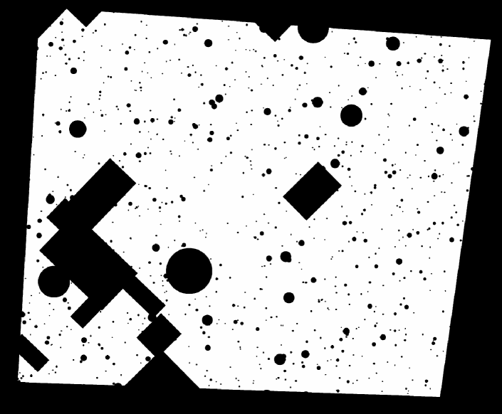
Figure 1.— Final region mask for the clustering analysis in the Lockman Hole field. The circles mark the locations of stars and bright objects. The rectangles mask those regions where the completeness of INT/WFC images is not achieved for $i=22.8$ (AB mag). All black patches were excluded from the subsequent analysis (see details in Section 2.2.1).

2.2.2 Identifying Low- and High-redshift Galaxy Populations

To derive the spatial correlation length and investigate the dependence of clustering on redshift, we need to know the redshift distribution of the sources. Unfortunately, the vast majority of the 24 $\mu\rm m$ sources selected in the Lockman Hole field have neither spectroscopic nor photometric redshifts. The SWIRE photometric redshift catalog (Rowan-Robinson et al., 2008), available in this field, has a limited and heavily inhomogeneous coverage for our sample. The approach we are taking instead is to use simple photometric criteria to divide the catalog into the low- and high-redshift subsamples, and then use a similarly selected sample of $24\,\mu\rm m$ sources from the GOODS survey to derive the redshift distribution within each subsample.

To separate the sample into low- and high-redshift sources, we defined the optical-to-NIR color selection criterion based on the optical $I$-band data (from ESIS-VIMOS survey; Berta et al., 2008) and SWIRE IRAC $4.5\,\,\mu\rm m$ observations in the ELAIS-S1 SWIRE field. Particularly, we examined the dependence of the $(I-[4.5])_{\rm AB}$ color on redshift for various galaxy spectral templates such as Mrk 231 (Sy-1), IRAS 19254 (Sy-2), M 82 (starburst), M 51 (spiral), and NGC 4490 (blue spiral) (see examples of a similar analysis in Berta et al., 2007, 2008). It appears that for starburst galaxies, the color cut $(I-[4.5])_{\rm AB}\sim 3$ separates well low ($z\lesssim 1$) and high ($z\gtrsim 1$) redshift galaxy populations, with only a small contamination in both groups. Such a rapid color transition around $z\sim 1$ can be explained by the passage of the Balmer break in the galaxy spectra through or redward the $I$ band.

To further refine this color selection criterion, we applied it to the deep Spitzer observations of GOODS fields (Rodighiero et al., 2010). The GOODS-N and GOODS-S $24\,\,\mu\rm m$ catalogs include 889 and 614 sources, respectively, detected in a total area of $\sim 350\,\text{arcmin$^{2}$}$. The catalogs are complete down to $S_{24\,\mu\rm m}=80\,\mu$Jy. Observations in the i band were made by the Advanced Camera for Surveys in both fields down to a magnitude limit i=26.5 (Grazian et al., 2006). Redshift estimates are available for all these sources, 46% are spectroscopic and 54% photometric redshifts. The latter are estimated with an rms scatter in $z_{\text{phot}}-z_{\text{spec}}$ of 0.09 and 0.06 for the GOODS-N and GOODS-S samples, respectively (for details see Rodighiero et al., 2010).

From the GOODS catalogs, we selected the sources with $S_{24\,\mu\rm m}>310\,\mu$Jy and separated them into two redshift bins $z>1.2$ and $z<1.2$. The color–magnitude diagram for these sources shows that the low- and high-$z$ galaxies indeed can be separated by a boundary value of $(i-4.5)=3$ (AB mag) (dashed line in Figure 2(a)). The deepest optical data available in the Lockman Hole field are those from the INT/WFC which provides sufficiently uniform coverage to $i=22.8$ (with the $5\sigma$ magnitude limit reaching $i=23.3$ (AB) in the deepest sections of the survey). Therefore, a magnitude cut of $i=22.8$ had to be incorporated in our selection. Figure 2(b) shows that the low-$z$ sources fainter than $i=22.8$ (above dotted line) and with the color $(i-4.5)<3$ (AB mag) (below dashed line) in practice are very few and they only minimally contaminate ($\sim 10\%$) the high-$z$ sample. Based on these considerations, we implemented the redshift separation as a combined color and magnitude criterion: the source is considered to belong to a high-redshift sample, if it is undetectable in the INT/WFC $i$ band, or its measured $i$ magnitude is $>22.8$, or the $(i-4.5)$ (AB mag) color is $>3$.

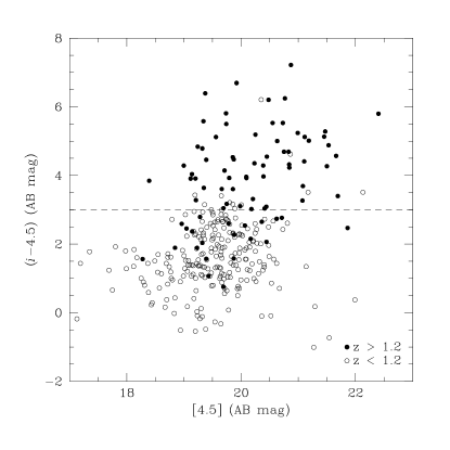
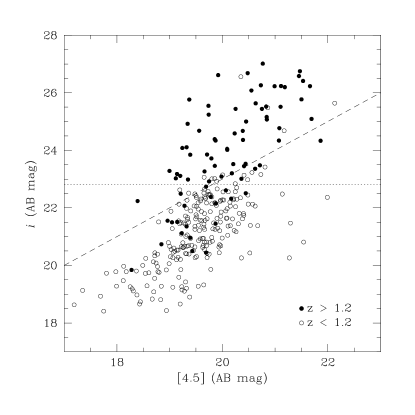
Figure 2.— Color–magnitude (a) and magnitude $i$ vs. magnitude [4.5] (b) diagrams for the GOODS-N and GOODS-S sources with $S_{24\,\mu\rm m}>310\,\mu$Jy. Open and filled circles are galaxies at redshifts lower and higher than $1.2$. On both figures, a dashed line represents $(i-4.5)=3$ (AB mag). A dotted line on the figure (b) corresponds to a magnitude $i=22.8$ at which the INT/WFC coverage is uniform in the Lockman Hole field.

One of the main sources of concern for the color–magnitude based separation of 24 $\mu\rm m$ objects into low- and high-redshift subsamples is the presence of active galactic nuclei (AGNs) in the sample. Therefore, we checked the AGN contents in the GOODS sample of the 24  $\mu\rm m$selected sources. According to Rodighiero et al. (2010), less than $10\%$ of these sources are type-1 AGNs. The authors classified the observed SEDs using Polletta et al. (2007) templates. This AGN fraction is consistent with that reported by Gilli et al. (2007) and Treister et al. (2006), who used very deep Chandra X-ray observations in the GOODS fields. Concerning the highly obscured (type-2) AGNs and the sources of composite spectral type (starburst+ANG), their contribution to the $24\,\,\mu\rm m$ emitting sources is hard to estimate. One of the reasons is that the AGN and star formation activity often occur simultaneously, and both are revealed in the form of the $24\,\,\mu\rm m$ emission (see, e.g., Brand et al., 2009; Rodighiero et al., 2010; Franceschini et al., 2005, and references therein). Some studies suggest, on the basis of estimates by different methods, that the $24\,\,\mu\rm m$ selected samples may contain $\sim$20%–30% of AGNs of both types (Sacchi et al., 2009; Franceschini et al., 2005). However, we note that to estimate the redshift distribution within our color and $i$-magnitude-selected subsamples, we used an empirical redshift distribution of identically selected GOODS sources (see below). As long as the GOODS redshifts are valid and the GOODS sample is a fair representation of our main Lockman Hole sample, the derived $dN/dz$ models for the low- and high-redshift subsamples are correct, even though the high-$z$ subsample may be slightly contaminated by AGNs.

2.3. Empirical Redshift Distributions

We need a model for the redshift distribution of the sources in order to use the Limber equation (Equations (3) and (9) below) to relate the angular and spatial correlation functions. We determined these redshift distributions empirically, using the GOODS sources selected identically to our main sample in the Lockman Hole field. All sources with $S_{24\,\mu\rm m}>310\,\mu$Jy in GOODS-N and GOODS-S fields were divided into low- and high-redshift subsamples by applying the color-magnitude selection criteria (Section 2.2.2 and Figure 2(b)). The obtained redshift distributions within these photometrically-selected samples are shown in Figure 3(a) and (b). These empirical distributions can be well approximated by a Gaussian model:

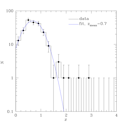
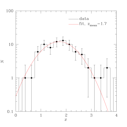
Figure 3.— Redshift distribution of GOODS sources ($S_{24\,\mu\rm m}>310\,\mu$Jy) incorporated into low-$z$ (a) and high-$z$ (b) subsamples based on their color $(i-[4.5])$ and $i$-band magnitude. Blue and red lines are Gaussian fits with $z_{\rm mean}=0.7$ and $z_{\rm mean}=1.7$, respectively.

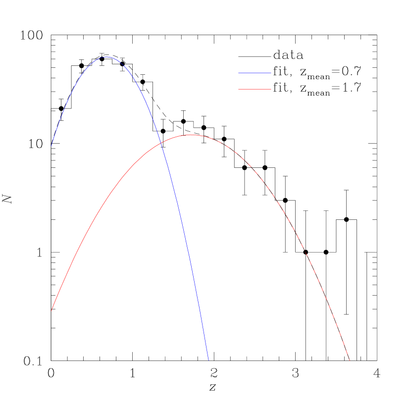
Figure 4.— Redshift distribution of sources brighter than $S_{24\,\mu\rm m}=310\,\mu$Jy from GOODS surveys. Blue and red lines are Gaussian fits to redshift distributions of sources undergone color–magnitude selection. The dashed line is a combined fit of two selected samples.

$$dN/dz=C\times\exp(-(z-z_{\text{mean}})^{2}/2\sigma^{2})$$ (1)

(blue and red lines in Figure 3). The best-fit parameters for the low-$z$ subsample in the redshift range $0<z<2$ are $C=50,\sigma=0.349,z_{\rm mean}=0.7$. For the high-$z$ subsample in the redshift range $0.5<z<3.5$, we find $C=12,\sigma=0.629,z_{\rm mean}=1.7$. The derived widths are significantly larger than the estimates uncertainties in the GOODS photometric redshifts ($\pm$0.06–0.09), and therefore accurately approximate the intrinsic widths of the redshift distributions for our two subsamples.

This two-Gaussian model provides a good fit also to the redshift distribution of all GOODS sources with $S_{24\,\mu\rm m}>310\,\mu$Jy (i.e., without the photometric separation into low and high-$z$ subsamples). The combined redshift distribution is shown in Figure 4, and the dashed line is the sum of two Gaussian models for the low and high-$z$ subsamples.

We also can use these subsamples of GOODS galaxies to estimate the typical infrared luminosities (8 $\mu\rm m$–1000 $\mu\rm m$) for our Lockman Hole sample. In the GOODS low-redshift subsample, $z_{\rm mean}=0.7$, the mean luminosity is $L_{\rm IR}\sim 3\times 10^{11}L_{{}_{\odot}}$ indicating that the selected objects belong to the class of luminous infrared galaxies (“LIRGs”, $10^{11}L_{{}_{\odot}}<L_{\rm IR}<10^{12}L_{{}_{\odot}}$, Sanders & Mirabel, 1996). The high redshift galaxies, $z_{\rm mean}=1.7$, have an order of magnitude higher mean luminosity, $L_{\rm IR}\sim 3\times 10^{12}L_{{}_{\odot}}$ which places them into the category of ultra-luminous infrared galaxies (“distant ULIRGs”; $L_{\rm IR}>10^{12}L_{{}_{\odot}}$; Sanders & Mirabel, 1996). Barring an unexpectedly high level of cosmic variance, our $24\,\mu\rm m$ sources selected in the Lockman Hole field should have the same mean luminosities.

3. Clustering properties of $24\,\,\mu\rm m$ selected galaxies

The total area of the Lockman Hole field used in the clustering analysis (white regions in Figure 1) is $\simeq 7.9$ deg². There are 21844   $24\,\mu\rm m$ emitting objects with fluxes greater than $310\,\mu$Jy within this area. Applying the color–magnitude selection criteria (Section 2.2.2), we obtained two subsamples of 14822 and 7022 sources with $z_{\rm mean}=0.7$ and $z_{\rm mean}=1.7$, respectively.

The angular correlation functions were estimated by the Landy & Szalay method (1993) at angular scales $0.01<\theta<3.5$ deg. The random points used in this estimator were homogeneously distributed in the field but avoiding the excluded regions of the mask shown in Figure 1. In order to suppress the uncertainties related to a complex geometry of the field and to decrease the statistical errors, the number of simulated random points was 100 times greater than the number of data points in each sample. The correlation function was computed in angular bins $\Delta\log\theta=0.2$. In Figure 5, we show the derived angular correlation functions for the whole sample (open black triangles), for the low-$z$ subsample with $z_{\rm mean}=0.7$ (open blue circles), and for high-$z$ subsample with $z_{\rm mean}=1.7$ (filled red circles).

Statistical uncertainties which can be assigned to angular correlation function $w(\theta)$ measured using the Landy & Szalay estimator are $\delta w(\theta)=1+w(\theta)/\!\!\sqrt{{\rm DD}(\theta)}$ (Landy & Szalay, 1993), where DD is the number of data pairs. However, it is considered that these uncertainties do not account for cosmic variance and covariance of the correlation function at different separations, and therefore, underestimate real errors. These difficulties might be overcome by applying, for instance, the jackknife subsampling of data (e.g., Scranton et al., 2002; Zehavi et al., 2002; Waddington et al., 2007; Ross et al., 2007). To calculate jackknife errors we divided the observed field into 25 approximately equal-sized patches and computed the correlation function excluding one part of our sample at one time. The ensemble errors are then estimated from the scatter between perturbed and full sample realizations:

$$\sigma^{2}(\theta)=\sum_{i=1}^{N}\frac{{\rm DR}_{i}(\theta)}{{\rm DR}(\theta)}[w_{i}(\theta)-w(\theta)]^{2},$$ (2)

where DR is the number of pairs between cross-correlated data and random catalogs, $i$ refers to a given sample realization, and ${\rm DR}_{i}/{\rm DR}$ accounts for a complex field geometry (Myers et al., 2005; Ross et al., 2007). All quoted uncertainties are obtained by applying the jackknife subsampling technique to the data, except in Appendix C, where we compare the correlation functions from different catalogs and calculate errors $\delta w(\theta)$ (see above).

Because of the good statistics of the SWIRE sample and the large size of the Lockman Hole field, we are able to measure the clustering signal at angular scales which correspond to fairly large spatial scales. Indeed, comoving sizes of 1–8 $h^{-1}\,$Mpc at $z=1.7$ correspond to an angular range of $0.017^{\circ}-0.13^{\circ}$. A great advantage of the measurements done at such large scales is that we directly probe the clustering signal at angular separations which correspond to the expected range of three-dimensional correlation lengths, $r_{0}$. This makes it possible to obtain robust estimates of $r_{0}$ from a standard power-law fit to the angular correlation function, $w(\theta)=(\theta/\theta_{0})^{1-\gamma}$, and application of the simplified Limber equation (full version is given by Equation (9)) which gives a direct link between the angular and spatial correlation lengths:

$$\theta_{0}^{\gamma-1}=r_{0}^{\gamma}\;A(\gamma){\displaystyle{\frac{2}{c}}}\;\frac{\int\limits_{0}^{\infty}dz\,N(z)^{2}\,H(z)D_{\rm M}(z)^{1-\gamma}}{\big{[}\int\limits_{0}^{\infty}dz\,N(z)\,\big{]}^{2}},$$ (3)

where $D_{\rm M}(z)$ is the transverse comoving distance to redshift $z$ and $N(z)$ is the redshift distribution of sample galaxies. $H(z)=H_{0}\sqrt{\Omega_{\rm M}(1+z)^{3}+\Omega_{k}(1+z)^{2}+\Omega_{\Lambda}}$ is the Hubble parameter at redshift $z$ and $A(\gamma)=\Gamma(1/2)\,\Gamma([\gamma-1]/2)/\Gamma(\gamma/2)$. If the angular correlation function measurements at large scales are unavailable, a power-law fit to the data at small angular/spatial scales may lead to incorrect estimates of the correlation lengths and incorrect conclusions about clustering properties of given galaxy populations (e.g., Kravtsov et al., 2004; Quadri et al., 2007, 2008, and references therein).

The angular correlation functions shown in Figure 5 were iteratively fitted over the angular range $0.01^{\circ}<\theta<3.5^{\circ}$ with a power-law model, $w(\theta)=(\theta/\theta_{0})^{1-\gamma}-{\rm IC}$, where the term IC refers to the Integral Constraint. The IC correction accounts for a systematic offset in estimated correlation function due to the finite size of any survey (Peebles, 1974, 1980) and it is usually calculated using a method proposed by Roche et al. (1993):

$${\rm IC}=\theta_{0}^{\gamma}\,\frac{\sum_{j}{\rm RR}(\theta_{j})\,\theta_{j}^{1-\gamma}}{\sum_{j}{\rm RR}(\theta_{j})},$$ (4)

where ${\rm RR}(\theta_{j})$ is the number of random pairs in an angular bin $j$.

The best-fit parameters for the entire sample are $\theta_{0}=0.31^{\prime\prime}\pm 0.04^{\prime\prime}$, and $\gamma=1.69\pm 0.11.$ Splitting the whole sample into smaller subsamples obviously increases the statistical uncertainties. Therefore, we decided to fix the power-law slope in the subsequent analysis at $\gamma=1.69$. The best-fit amplitudes for the low-$z$ and high-$z$ data are then $\theta_{0}=0.63^{\prime\prime}\pm 0.09^{\prime\prime}$ and $\theta_{0}=0.91^{\prime\prime}\pm 0.21^{\prime\prime}$, respectively. These best-fit models are shown in Figure 5 with blue and red dotted lines.

The spatial correlation lengths $r_{0}$ were then obtained from the Limber inversion (Equation (3)) using the fits to the empirical redshift distributions of GOODS survey sources, described in Section 2.3. The derived correlation lengths are $r_{0}=4.98\pm 0.28\,h^{-1}\,$Mpc (comoving) for the low-$z$ ($z_{\rm mean}=0.7$), and $r_{0}=8.04\pm 0.69\,h^{-1}\,$Mpc for the high-$z$ ($z_{\rm mean}=1.7$) sample. Without using a fixed power-law slope, we obtain $r_{0}=5.07\pm 0.34\,h^{-1}\,$Mpc, $\gamma=1.63\pm 0.11$, and $r_{0}=7.99\pm 0.75\,h^{-1}\,$Mpc, $\gamma=1.65\pm 0.20$, for the low and high-$z$ subsamples, respectively.

The uncertainties above include only statistical errors in the measurement of the angular correlation function. In principle, another source of uncertainty is the inaccuracies in the models for the redshift distribution. These are hard to estimate in our case since we use an empirical fit to the $dN/dz$ observed for the GOODS sources and any inaccuracies would be related to problems with the GOODS photometric redshifts. The range of theoretical models for the redshift distribution of 24  $\mu\rm m$ sources provides a poor guidance because these models, still poorly constrained by observations, sometimes give contradictory results (Desai et al., 2008; Rowan-Robinson et al., 2008; Franceschini et al., 2010). Qualitatively, if the real $dN/dz$ distribution for our sources is wider than what we assume, the correlation lengths should be corrected upward.

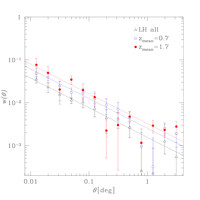
Figure 5.— Two-point angular correlation function of SWIRE Lockman Hole sources brighter than $S_{24\,\mu\rm m}=310\,\mu$Jy. The dotted lines are power-law fits. Triangles represent clustering of the whole sample, open and filled circles are for the low-$z$ and high-$z$ galaxies, respectively.

As a further check, we re-estimated the correlation lengths for our high-$z$ subsample using the redshift distribution of the 24  $\mu\rm m$ sources in the COSMOS field (Sanders et al., 2007; Le Floc’h et al., 2009; Ilbert et al., 2009). The COSMOS survey area is significantly larger than GOODS ($\approx$2 deg² versus $\approx$0.1 deg²) and thus is more representative of our Lockman Hole region. Unfortunately, there are two problems which prevent us from using the COSMOS $dN/dz$ as our baseline model. First, the optical and near-IR data in the COSMOS field are shallower than those in GOODS, which can affect the $dN/dz$ distribution at high redshifts. Indeed, 7% of the COSMOS 24  $\mu\rm m$ sources with $S_{24\,\mu\rm m}>310\,\mu$Jy have no redshifts; this is $\approx$20% of the sources in our high-$z$ bin. Second, there is a significant overdensity of galaxies at $z\sim 1$ in the COSMOS field (de la Torre et al., 2010). However, even with these problems in mind, using the COSMOS-derived $dN/dz$ for the estimates of $r_{0}$ from the Limber equation provides a useful test of sensitivity of our results to the assumed shape of the redshift distribution, possible cosmic variance in the GOODS field, etc. We applied the same color–magnitude criteria to the 24  $\mu\rm m$ COSMOS sources and approximated the redshift distribution for the high-$z$ bin using either a single-Gaussian model as we do for GOODS, or two-Gaussian model to better fit a component near $z\sim 1$. We derive $r_{0}=7.90\,h^{-1}\,$Mpc and $8.23\,h^{-1}\,$Mpc for these two $dN/dz$ approximations, respectively; these values are to be compared with $r_{0}=8.04\pm 0.69\,$Mpc we derive using the GOODS $dN/dz$. Therefore, this test confirms that the uncertainties in $r_{0}$ related to the redshift distribution of sources are small compared to the purely statistical uncertainties.

In what follows, we use the derived correlation lengths for the 24  $\mu\rm m$ selected galaxies for estimating the mass range of their host DM halos through the comparison of our measurements with the clustering properties of DM halos from the Bolshoi cosmological simulation (Klypin et al., 2011).

4. Properties of dark matter halos hosting $24\,\,\mu\rm m$ selected galaxies

4.1. Galaxy Population Model

Several methods can be used to connect a population of galaxies with that of their host DM halos (see, e.g., Guo et al., 2010, and references therein). Here, we use the clustering properties, assuming that the mass scale of the DM halos hosting the galaxies can be established by requiring that the observed correlation function of galaxies selected above a luminosity threshold matches the correlation function of DM halos selected above a certain mass limit (Kravtsov et al., 2004; Conroy et al., 2006) .

To compute the correlation function of the DM halos, we used the outputs of the Bolshoi cosmological simulation for redshifts ranging from 0.5 to 2.5 with a step size of $\Delta z=0.5$. The Bolshoi simulation, described in Klypin et al. (2011), is a high-resolution and large-volume run performed with the WMAP5 and WMAP7 cosmological parameters $\Omega_{\rm M}=0.27$, $h=0.7$, and $\sigma_{8}=0.82$ (Komatsu et al., 2009, 2011). The simulation contained $2048^{3}\approx 8$ billion DM particles in a $250\,h^{-1}\,$Mpc box. The corresponding mass and force resolutions are $m_{p}=1.35\times 10^{8}\,h^{-1}\,M_{\odot}$ (one particle mass) and $1.0\,h^{-1}\,$kpc (the smallest cell size in physical coordinates), respectively. The simulation outputs were recorded at 180 time steps and were analyzed by the halo-finding algorithm (Klypin & Holtzman, 1997; Kravtsov et al., 2004; Klypin et al., 2011) to locate gravitationally bound objects and to calculate their characteristics such as the virial mass $M_{\rm vir}$, virial radius $R_{\rm vir}$, maximum circular velocity $v_{\rm max}$, etc. The identified halos are classified into distinct (host, parent) halos whose centers are not located within any larger virialized systems, and subhalos (satellites, substructure) which lie within the virial radius of a larger halo. The completeness limit for the halo catalogs derived from the Bolshoi outputs is $v_{\rm max}=50$ km s^-1 or $M_{\rm vir}\approx 1.5\times 10^{10}\,h^{-1}\,M_{\odot}$.

As outlined in Kravtsov & Klypin (1999), Nagai & Kravtsov (2005), and Conroy et al. (2006), the maximum circular velocity, $v_{\rm max}$, of a DM halo, rather than its virial mass, is more closely related to the properties of a galaxy residing in this halo. Therefore, we “populated” the Bolshoi simulation with “galaxies” by putting the “galaxies” at the centers of all halos and subhalos selected above a given $v_{\rm max}$ threshold (this threshold value of $v_{\rm max}$ is referred to as $V_{\rm min}$ hereafter). The considered range of $V_{\rm min}$ is $130<V_{\rm min}<385\,$km s^-1. The lower velocity limit is chosen so that the correlation length for such DM halos is below the $r_{0}$ derived for our low-$z$ subsample of 24  $\mu\rm m$ galaxies. The high velocity limit is chosen to ensure that the statistics of DM halos is sufficiently good at all output redshifts of the Bolshoi simulation. We estimated the correlation lengths for the model galaxy populations by fitting their spatial correlation functions with a power law at scales $1<r<25\,h^{-1}\,$Mpc.

Figure 6.— Spatial correlation length of dark matter halos as a function of the maximum circular velocity threshold and redshift.

Figure 6 shows the derived model correlation lengths for DM halos as a function of $V_{\rm min}$ and redshift. Clearly, the $r_{0}$ significantly increases with $V_{\rm min}$ (or mass) of the halos and also changes with redshift. These correlation lengths can be matched to the observed $r_{0}$ for our samples of 24  $\mu\rm m$ selected galaxies. The redshifts of the simulation outputs do not match exactly the mean redshifts of our galaxy samples, $z_{\rm mean}=0.7$ and $z_{\rm mean}=1.7$. However, the trend of the model $r_{0}$ with $z$ for a given $V_{\rm min}$ is weak, and so we can linearly interpolate between the results for the outputs branching the mean redshifts in the data.

4.2. Halo Mass and Number Density

Using these data, each observed value of $r_{0}$ can be matched to the corresponding $V_{\rm min}$. The uncertainty intervals for our low- and high-$z$ subsamples, $r_{0}=4.98\pm 0.28\,h^{-1}\,$Mpc and $r_{0}=8.04\pm 0.69\,h^{-1}\,$Mpc, respectively, correspond to $V_{\rm min}$ intervals of $V_{\rm min}=172\pm 18\,$km s^-1 for low-$z$ $24\,\,\mu\rm m$ galaxies and $V_{\rm min}=322\pm 33\,$km s^-1 for the high-$z$ subsample with $z_{\rm mean}=1.7$.

These velocity thresholds can be easily converted to the corresponding virial mass limits, $M_{\rm vir}$, using a tight scaling, which approximately goes as $v_{\rm max}\propto M^{1/3}_{\rm vir}$ (e.g., Klypin et al., 2011). This relation is valid for both distinct halos and subhalos at different redshifts. Fitting the $v_{\rm max}-M_{\rm vir}$ relation for all halos and subhalos above $v_{\rm max}>130\,$km s^-1 in the Bolshoi outputs, we obtain the following power-law scalings:

$$\log M_{\rm vir}=4.60+3.25\,\log v_{\rm max}, \text{for$z=0.5$},$$ (5)

$$\log M_{\rm vir}=4.69+3.13\,\log v_{\rm max}, \text{for$z=1.5$},$$ (6)

where $M_{\rm vir}$ is in units of $h^{-1}\,M_{{}_{\odot}}$. These results can be scaled to the mean redshifts of our samples using the expected redshift evolution of the $v_{\rm max}-M_{\rm vir}$ relation, which goes as $M_{\rm vir}\propto E(z)^{-1}$ for a fixed $v_{\rm max}$ (Borgani & Kravtsov, 2011), where $E(z)=H(z)/H_{0}$. Using these scalings, we find that the limiting total mass for the $24\,\,\mu\rm m$ emitting galaxies with $z_{\rm mean}=0.7$ is $M_{\rm tot}=(0.7\pm 0.2)\times 10^{12}\,h^{-1}\,M_{\odot}$ and $M_{\rm tot}=(3.1\pm 1.0)\times 10^{12}\,h^{-1}\,M_{\odot}$ for our high-$z$ sample.

Having this established mass scale, we can approximately estimate the fraction of massive DM halos containing 24  $\mu\rm m$ emitting galaxies, even though our sample is not volume-limited. The observed comoving number density of the galaxies near the mean redshift of the sample can be estimated as

$$n_{\rm gal}=\frac{dN/dz}{dV/dz}=1.1\times 10^{-3}\,h^{3}\,{\rm Mpc^{-3}}, \text{$z_{\rm mean}=0.7$},$$ (7)

$$n_{\rm gal}=0.12\times 10^{-3}\,h^{3}\,{\rm Mpc^{-3}}, \text{$z_{\rm mean}=1.7$},$$ (8)

where $dV/dz$ is the comoving volume within the survey area. These values are compared with the number density of halos in the Bolshoi outputs above the derived $V_{\rm min}$ thresholds. For $z=0.5$, $v_{\rm max}>172\,$km s^-1, we find $n_{\rm halo}=5.0\times 10^{-3}\,h^{3}\,{\rm Mpc^{-3}}$, or $n_{\rm halo}\approx 5\,n_{\rm gal}$. For $z=1.5$, $v_{\rm max}>322\,$km s^-1, the corresponding number densities are $n_{\rm halo}=0.48\times 10^{-3}\,h^{3}\,{\rm Mpc^{-3}}$ or $n_{\rm halo}\approx 4\,n_{\rm gal}$. Therefore, we find that similar fractions, $\sim 20\%$, of DM halos contain galaxies with $S_{24\,\mu\rm m}>310\,\mu$Jy at both low and high redshifts. This may be simply a coincidence since the mass and 24  $\mu\rm m$ luminosity scales for the two samples are quite different and so we cannot separate the luminosity and redshift dependences.

4.3. Full Limber Modeling of the Observed Angular Correlation Function

Finally, we test that our analysis based on the power-law approximation of the observed angular correlation functions provides unbiased answers even though the correlation function of DM halos shows clear deviations from the power law at both small and large scales (Kravtsov et al., 2004; Springel et al., 2005). For this, we compute a full projection of the two-point spatial correlation function of the Bolshoi DM halos for $v_{\rm max}>172\,$km s^-1 at $z=0.5$ and $v_{\rm max}>322\,$km s^-1 at $z=1.5$. The spatial correlation functions, $\xi(r)$, for the halos were calculated at scales $0<r<50\,h^{-1}{\rm Mpc}$ in narrow, $\Delta\log r=0.1\,h^{-1}{\rm Mpc}$, bins, and then were used in the full Limber (1953) transformation:

$$w(\theta)={\displaystyle{\frac{2}{c}}}\;\frac{\int\limits_{0}^{\infty}dz\,N(z)^{2}\,H(z)\int\limits_{0}^{\pi_{\rm max}}d\pi\,\xi\left(\!\sqrt{[D_{\rm M}(z)\theta]^{2}+\pi^{2}}\right)}{\big{[}\int\limits_{0}^{\infty}dz\,N(z)\,\big{]}^{2}},$$ (9)

where the functions are the same as in Equation (3), and $\xi(r)=\xi\left(\!\sqrt{[D_{\rm M}(z)\theta]^{2}+\pi^{2}}\right)$ is the three-dimensional correlation function under approximation of small angles ($\theta\ll 1$  [rad]), $\pi$ is the radial separation. The results are shown in Figure 7. The blue and red data points (open and filled circles, respectively) show the observed angular correlation functions for the low-$z$ and high-$z$ samples (same as those in Figure 5), and the lines are the full projections of the halo correlation functions for the best fit values of $V_{\rm min}$.

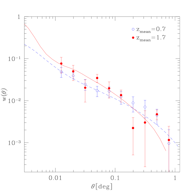
Figure 7.— Observed two-point angular correlation function for low-$z$ (open circles) and high-$z$ (filled circles) samples of the $24\,\,\mu\rm m$ selected galaxies. The dashed and solid lines are the angular correlation function models derived from the full Limber inversion of spatial correlation functions of DM halos with maximum circular velocities greater than $V_{\rm min}=172\,\,{\rm km\,\,s^{-1}}$ and $V_{\rm min}=322\,\,{\rm km\,\,s^{-1}}$.

Clearly, the full models fit the data points very well, confirming that the power-law approximation to the observed $w(\theta)$ yields accurate estimates of the spatial correlation lengths, $r_{0}$, and thus accurate mass scales for the DM halos hosting the 24  $\mu\rm m$selected galaxies. At $\theta>0.2$ deg we observed a decline of the observed correlation functions relative to the power-law approximations, and this could be related to the behavior of the DM halos correlation function at large scales (e.g., Springel et al., 2005, and model curves in Figure 7) .

At the opposite end, $\theta<0.01$ deg, the models show enhancements in the clustering signal relative to the power-law extrapolation from large radii. These enhancements correspond to the correlation function of galaxies located within a single parent halo (the so-called “one-halo” term, Cooray & Sheth, 2002; Kravtsov et al., 2004). The measurements of the correlation function at these scales are very interesting because they can be used to determine the location of galaxies in the host DM halos, and thus to constrain their recent merger history (e.g. Porciani & Giavalisco, 2002; Lee et al., 2006; Quadri et al., 2008; Cooray et al., 2010). Unfortunately, the broad PSF of the MIPS instrument does not allow us to make reliable measurements of the clustering of 24  $\mu\rm m$ sources at such small scales (see discussion in Appendix C).

5. Comparison with previous measurements

It is important to compare our measurements with the previous studies of the clustering properties of $24\,\mu\rm m$ selected galaxies. In doing so, we should keep in mind that direct comparisons with other studies are difficult because of a wide variety of criteria used for selecting high-redshift sources. The comparison presented below is done in terms of the correlation lengths. We do not compare the derived halo masses because their estimates depend on the assumptions on the cosmological parameters, power spectrum, and halo occupation models (e.g., Conroy et al., 2008), and even the definition used (e.g., threshold versus mean mass for a population).

We start with low-redshift ($z<1$) samples selected in small areas. Gilli et al. (2007) presented the correlation function measurements of the $S_{24\,\mu\rm m}>20\,\mu$Jy galaxies with the mean $z\sim 0.8$, detected in the GOODS fields. They found that the correlation length increases with the infrared luminosity, reaching for LIRGs ($L_{\rm IR}>10^{11}L_{{}_{\odot}}$) a level of $r_{0}=5.14\pm 0.76\,h^{-1}$ Mpc. Our estimate of $r_{0}$ for the low-z subsample ($z_{\rm mean}=0.7$) is almost identical to this value. Another study, focused on the bright $24\,\mu\rm m$ emitting galaxies, was performed by Magliocchetti et al. (2008). The galaxies brighter than $S_{24\,\mu\rm m}=400\,\mu$Jy detected in the SWIRE XMM-LSS field ($0.7{\rm deg}^{2}$ used in the analysis) were divided into low-redshift (350 sources at $z_{\rm mean}=0.79$) and high-redshift (210 objects at $z_{\rm mean}=2.02$) subsamples based on photometric redshifts. The samples are thus comparable to those selected in our work. The derived correlation lengths were $5.9^{+1.1}_{-1.3}\,h^{-1}$Mpc and $11.1^{+2.0}_{-2.4}\,h^{-1}$Mpc for the low and high-$z$ subsamples, respectively. Within uncertainties, these results are in a reasonable agreement with our measurements. However, our sample contains a much larger number of sources and covers a wider area, so we were able to measure the angular correlation function at larger scales (probing directly the “two-halo” term, e.g., Cooray & Sheth, 2002) and significantly reduce the statistical uncertainties.

Several studies were focused on distant ULIRGs ($z\sim 2$) but they used selection criteria in addition to $24\,\mu\rm m$ flux (Farrah et al., 2006; Magliocchetti et al., 2007; Brodwin et al., 2008), therefore their and our results should be compared with caution. For example, Farrah et al. (2006) used a sample of the ULIRGs with $S_{24\,\mu\rm m}>400\,\mu$Jy which also had a spectral peak in the $4.5\,\mu\rm m$ and $5.8\,\mu\rm m$ IRAC bands, corresponding to the redshifted stellar $1.6\,\mu\rm m$ peak. The $4.5\,\mu\rm m$ peak sources were estimated to be at $1.5<z<2.0$; their derived correlation length was $r_{0}=9.40\pm 2.24\,h^{-1}\,$Mpc. The $5.8\,\mu\rm m$ peak sources are at $2<z<3$ and their angular clustering corresponded to the correlation length of $r_{0}=14.40\pm 1.99\,h^{-1}\,$Mpc. The Farrah et al. $r_{0}$ for the 24 $\mu\rm m$+4.5 $\mu\rm m$ peak sample is higher than (but consistent within the errors) our value for the high-$z$ sample. We note that their results (as well as those of Magliocchetti et al., 2008) are dominated by the angular clustering measurements at small scales, and thus can be biased if one uses a power-law fit for the angular correlation function (Kravtsov et al., 2004; Quadri et al., 2007). In another work, a sample of dust obscured galaxies (“DOGs”; Dey et al., 2008) was selected. DOGs are mid-IR luminous ($S_{24\,\mu\rm m}>300\,\mu$Jy) and optically faint ($R-[24]>14$) galaxies estimated to be at $z\sim 2$. Their measured correlation length is $7.4^{+1.27}_{-0.84}\,h^{-1}\,$Mpc (Brodwin et al., 2008), similar to our value.

Models of galaxy formation suggest that DOGs and submillimeter galaxies (“SMGs”; Blain et al., 2002) form by mergers of massive ($M_{\rm tot}\sim 10^{12-13}\,h^{-1}M_{\odot}$) galaxies (see Narayanan et al., 2010, and references therein) and may represent different phases in the evolution of a merging system. It would be interesting to compare the clustering of SMGs and other classes of ULIRGs, but, unfortunately, the present estimates of the SMG correlation length is too uncertain (Blain et al., 2004; Scott et al., 2006; Weiß et al., 2009; Viero et al., 2009; Maddox et al., 2010; Cooray et al., 2010; Amblard et al., 2011). The best available measurements for submillimeter sources with redshifts close to our high-$z$ subsample have been presented in Cooray et al. (2010). The authors reported a clustering strength of $r_{0}=3.15\pm 0.35\,h^{-1}$Mpc and $r_{0}=4.41\pm 0.49\,h^{-1}$Mpc for the HerMes-Herschel sources detected down to the 30 mJy at $250\,\mu\rm m$ and $500\,\mu\rm m$. The mean redshift of the samples are $z_{\rm mean}^{250}\approx 2.1$ and $z_{\rm mean}^{500}\approx 2.6$. It is unlikely that these sources are directly related to our $24\,\mu\rm m$ selected galaxies because of very different values of the inferred correlation lengths.

6. Conclusions

We presented an analysis of the clustering properties of $24\,\mu\rm m$ emitting ($S_{24\,\mu\rm m}>310\,\mu$Jy) galaxies detected in Lockman Hole—one of the largest fields in the Spitzer/SWIRE survey. The large number of sources ($\sim 20,000$) and the size of the field allowed us to detect the clustering signal with high level of significance and probe large angular scales. Due to the lack of direct redshift measurements for the objects in the Lockman Hole sample, we used the optical and near-IR photometric data to separate the sample into high-redshift and low-redshift galaxies. The selection criteria as well as the redshift distributions for color-separated subsamples were empirically established using the catalogs of GOODS $24\,\mu\rm m$ sources (Rodighiero et al., 2010), whose redshifts were measured spectroscopically or estimated from multiband photometry. Using a power-law approximation to the correlation function, we derived the spatial correlation length $r_{0}$. We found $r_{0}=4.98\pm 0.28\,h^{-1}\,$Mpc and $r_{0}=8.04\pm 0.69\,h^{-1}\,$Mpc for $z_{\rm mean}=0.7$ and $z_{\rm mean}=1.7$ populations, respectively.

The estimated infrared luminosities showed that our $24\,\mu\rm m$ selected galaxies belong to populations of distant ULIRGs and local LIRGs. Based on the clustering analysis, we can conclude that our $24\,\mu\rm m$ selected galaxies represent different populations of objects found in differently sized DM halos, $M_{\rm tot}\gtrsim 7\times 10^{11}\,h^{-1}\,M_{\odot}$ and $M_{\rm tot}\gtrsim 3\times 10^{12}\,h^{-1}\,M_{\odot}$ at low and high redshifts, respectively. In each case, the $24\,\mu\rm m$ selected galaxies populate $\sim 20\%$ of the halos at these mass thresholds. Their high level of mid-IR luminosities may be caused by similar physical processes (e.g., triggered by mergers or interactions), but occurring in different environments. Further information can be obtained by studying in detail the dependence of clustering properties on the IR luminosity at each redshift.

Below, we present a study of stability of the correlation function measurements for $24\,\mu\rm m$ sources through comparison of different source catalogs in the SWIRE fields. In particular, we use four largest SWIRE fields (Lockman Hole, ELAIS-N1, ELAIS-N2, CDFS) and three catalogs - two versions of the SWIRE team catalogs (produced in 2005 and 2010, respectively) and our own list of sources extracted from Spitzer-MIPS maps using the wavelet decomposition method (Vikhlinin et al., 1998).

Appendix A Catalogs of $24\,\mu\rm m$ Sources

The first data set we used is publicly available catalogs from the SWIRE Data Release 2 (version 2005). These catalogs consist of the optical, IRAC, and MIPS 24  $\mu\rm m$ information merged into a single table for sources detected in the IRAC 3.6 and 4.5  $\mu\rm m$ bands above pre-defined SNR thresholds. Source detection in the MIPS data was carried out using SExtractor (Bertin & Arnouts, 1996). The estimated completeness threshold is $\sim 400\,\mu$Jy in all fields. For the clustering analysis, we selected all $24\,\,\mu\rm m$ sources above this flux threshold. To eliminate Galactic stars (see Section 2.2.1), we cross-correlated this set of 24  $\mu\rm m$ sources with the objects in the 2MASS survey using a matching radius of $2.5^{\prime\prime}$. Hereinafter, we refer to these source catalogs (with stars eliminated) as the “2005-catalog” or “v.2005”.

The second set of catalogs is based on the SWIRE Final Data Release (J. A. Surace et al. in preparation), a re-reduction of both the IRAC and MIPS datasets reaching a fainter flux limit. Ancillary multi-wavelength photometry from the FUV to the NIR was compiled for sources detected at either $3.6\,\,\mu\rm m$ or $4.5\,\,\mu\rm m$ into the so-called Data Fusion (M. Vaccari et al., in preparation). For the IRAC images, the source detection was again done using SExtractor, while the MOPEX/APEX package (Makovoz & Marleau, 2005) was used for MIPS data. The MOPEX/APEX package was specifically optimized for detection of point-like sources in crowded fields, and its application results in a significant improvement in the completeness limit for MIPS data, which can be as low as $\sim 200\,\mu$Jy (see below). The completeness of the IRAC detections was also improved compared to the previous data release. The initial IRAC source was associated with the data from other catalogs (e.g., the 2MASS PSC) using a matching radius of $2.5^{\prime\prime}$. In order to avoid source confusion and false identification in the $24\,\,\mu\rm m$ band, Vaccari et al. matched $24\,\,\mu\rm m$ and IRAC sources within the same radius of $2.5^{\prime\prime}$. For our analysis, we used all these $24\,\,\mu\rm m$ sources, and the selected sample is referred to as the “2010-catalogs” or “v.2010”.

Another significant difference between the 2005- and 2010-catalogs is in the methods of flux measurements for the MIPS sources. The 2005 data release used the aperture photometry with a set of apertures $7.5^{\prime\prime}-15^{\prime\prime}$ radius, which contained $60\%-85\%$ of the total flux, and applying suitable aperture corrections as determined by the MIPS instrument team. The MOPEX/APEX package yields the total fluxes provided by the PSF fitting. This is significant in our case because the aperture and PSF fitting photometry have different problems in dealing with the close source pairs, which can produce different results for the small-scale clustering.

Because, as we show below, neither the 2010- nor 2005- catalogs are completely free of problems, we produced our own list of MIPS-detected sources (see Section 2.1 for details). This third data set is referred to as the “A1-catalog” below.

All $24\,\mu\rm m$-IRAC catalogs were cross correlated with the 2MASS survey (Skrutskie et al., 2006) in order to identify and remove foreground stars using Shupe et al. (2008) criterion and to built region masks (Section 2.2.1). It appeared that in general Galactic stars comprise $\sim 2\%$ to the total number of sources detected in the $24\,\mu\rm m$-IRAC bands of SWIRE images.

Appendix B Limiting Fluxes for Individual Catalogs

For a proper comparison of the angular correlation function between different versions of the source catalogs and different fields, we have to make sure that the sources are selected above a flux which exceeds a completeness limit for each field/catalog. Ideally, a completeness limit is a flux threshold above which (nearly) all real sources are detected and into which (almost) no fainter sources migrate. The exact completeness limit for the MIPS/SWIRE data can be established only through Monte Carlo simulations (e.g., Shupe et al., 2008). However, we can apply a useful empirical criterion and identify the sensitivity limit with a point of maximum in the differential $\log N$ – $\log S$ distribution observed for each field/catalog.

In Figure 8, we show the number of sources per square degree and the logarithmic flux bin contained in the 2010-catalogs for different SWIRE fields. The maxima in the differential $\log N$ – $\log S$ distribution in all cases are achieved near a flux of $\sim 200\,\mu$Jy. However, there are clear differences in the number counts of faint sources up to a flux limit of $S_{24\,\mu\rm m}\sim 350\,\mu$Jy. This probably indicates a flux measurement uncertainty of $\sim 100\,\mu$Jy, which may explain also why the drop in the differential $\log N$ – $\log S$ distribution below the point of maximum is not sharp but extends to $\sim 100\,\mu$Jy. Therefore, based on examination of the $\log N$ – $\log S$ distributions, the correlation functions for the 2010-catalog in different SWIRE fields should be compared for sources brighter than $350\,\mu$Jy.

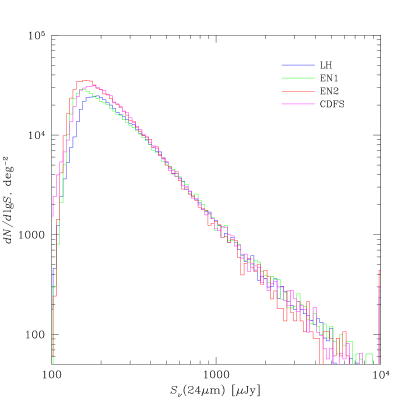
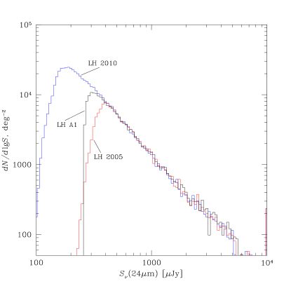
Figure 8.— Number of $24\,\mu\rm m$ sources per square degree per $\log$-flux interval plotted vs. the logarithmic flux. Left: the sources were selected from the 2010-catalogs (M. Vaccari et al., in preparation) in the four SWIRE fields—Lockman Hole (blue), ELAIS-N1 (green), ELAIS-N2 (red), and CDFS (magenta). Galactic stars were masked out and eliminated. Right: the sources were selected from three catalogs in the Lockman Hole. Blue, red, and black lines are for 2010-, 2005- and A1-catalogs, respectively.

Table 1Properties of MIPS SWIRE Fields

Field	$S_{\rm lim}$ ($\mu$Jy)	Area ($\rm deg^{2}$)
	$S^{2010}=180$
Lockman Hole	$S^{2005}=400$	$8.7$
	$S^{\rm A1}=310$
ELAIS-N1	$160$	$7.1$
ELAIS-N2	$170$	$3.3$
CDFS	$180$	$6.2$
ELAIS-S	$S^{\rm A1}=400$	6.3

Note. — The limiting fluxes, $S_{\rm lim}$, reported here correspond to the maxima in the source count histograms in Figure 8.

In Figure 8, we show the source counts for the three different catalogs in the Lockman Hole field. There is a striking difference in the sensitivity limits between the 2005 and 2010 versions of the SWIRE team catalogs—the maxima in the differential $\log N$ – $\log S$ distributions are at $S_{24\,\mu\rm m}=400$ and $180\,\mu$Jy, respectively. The sensitivity limit for the A1-catalog is between these two values, at $\approx 310\,\mu$Jy. Note that the drop in number counts below the maximum is very sharp for the A1-catalog, indicating a high level of reliability for the flux measurements. Even though the $\log N$ – $\log S$ for the 2010-catalog extends further down, the flux region $S_{24\,\mu\rm m}\lesssim 350\,\mu$Jy in this catalog might be affected by the scatter in the source flux measurements, as we have just discussed.

The sensitivity limits (the points of maxima in the differential $\log N$ – $\log S$ distribution) for different fields and catalogs are reported in Table 1 together with the field areas after applying the stellar mask (see discussion in Section 2.2.1). Below, we compare the angular correlation function computed for different fields/catalogs taking into account these sensitivity limits.

Appendix C Comparison of the Angular Correlation Functions

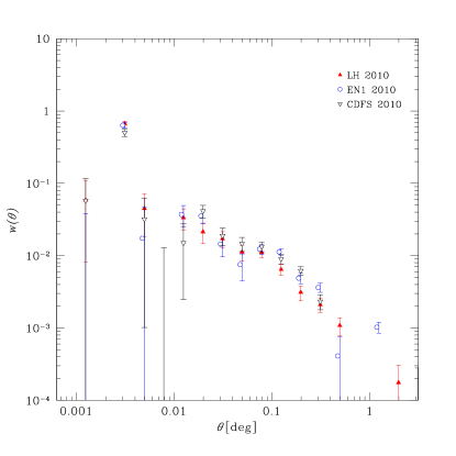
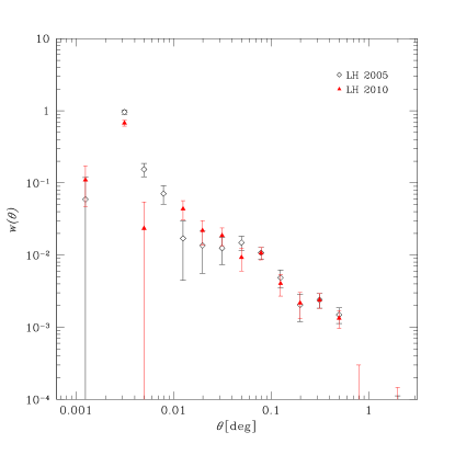
Figure 9.— Left: angular correlation function for sources from 2010-catalogs with fluxes brighter than $S_{24\,\mu\rm m}=350\,\mu$Jy detected in the Lockman Hole (red filled triangles), ELAIS-N1 (blue open circles), and CDFS (black open triangles). Right: comparison of the angular correlation functions in the Lockman Hole field using the sources from the 2010- and 2005-catalogs with $S_{24\,\mu\rm m}>400\,\mu$Jy.

We start with a comparison of the angular correlation functions, $w(\theta)$, computed for different SWIRE fields using the 2010-catalog. As discussed above, we use a flux threshold of $350\,\mu$Jy. This is the flux above which the $\log N-\log S$ distributions agree among different fields (Figure 8), and it is higher than the formal sensitivity limit for the 2010-catalogs. The results are shown in Figure 9 (left). Reassuringly, there is an excellent agreement between the results in different fields. At the largest separations, $\sim 1^{\circ}$ and above, the angular correlation function becomes consistent with zero, but one might expect distortions at such large scales because they are comparable to the size of the fields we are using. More relevant to our analysis are the obvious problems at small scales. There is a drop in the correlation signal at $0.003^{\circ}<\theta<0.01^{\circ}$, and a strong positive signal located in a single bin at $\theta\sim 0.003^{\circ}$. As we discuss below, these distortions are probably related to blending of nearby sources due to a relatively large size of the MIPS PSF.

Next, we compare the correlation functions for the 2005- and 2010-catalogs above the sensitivity limit for v.2005 ($400\,\mu$Jy). The results for the Lockman Hole field are shown in Figure 9 (right). There is a good agreement at large scales ($\theta\gtrsim 0.02^{\circ}$) but a strong difference at small scales. While there is a drop in the correlation signal at $0.003^{\circ}<\theta<0.01^{\circ}$ for the 2010-catalog sources, there is a strong excess correlation in the same angular range for the v.2005 sources. The origin of the discrepancy is probably not because some real pairs at separations of $\sim 30^{\prime\prime}$ are missing from the 2010-catalog—it is highly unlikely that this, more sensitive source list would miss any sources brighter that $400\,\mu$Jy. Rather, we suggest that some of these close pairs arise spuriously in the 2005-catalog because high fluxes are erroneously assigned to some faint sources in the vicinity of bright ones (see also Surace et al., 2005).

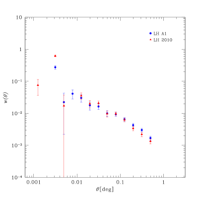
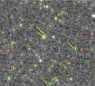
Figure 10.— Left: angular correlation function of $24\,\mu\rm m$ sources from the 2010 (red filled triangles) and A1 (blue filled circles) catalogs using a flux limit of $S_{24\,\mu\rm m}=310\,\mu$Jy in both cases. Right: comparison of the bright sources, $S_{24\,\mu\rm m}>310\,\mu$Jy, in the 2010- and A1-catalogs (green and red circles, respectively) in a subsection of the Lockman Hole field. Blue arrows point to real detections which are not present simultaneously in two catalogs. Yellow arrows indicate spurious detections in the 2010-catalog arising in proximity of bright/extended sources.

Next, we compare the results for the Lockman Hole field using the sources from the 2010- and A1-catalogs above a flux threshold of $S_{24\,\mu\rm m}=310\,\mu$Jy, the sensitivity limit of the A1- catalog. The results are shown in Figure 10 (left). The measurements are nearly identical at scales $\theta>0.01^{\circ}$, but the A1 correlation function shows somewhat weaker small-scale distortions. This impression is confirmed by cross-examination of the source detections from both catalogs overlayed on the input MIPS image (Figure 10 (right)). Most sources are found in both catalogs. There are a small number of real sources contained in one catalog but not the other (examples are marked by blue arrows) but this is not surprising because the source fluxes are derived using different methods and so we can expect some “migration” across the flux threshold. However, there are some cases (marked by yellow arrows) where obviously spurious sources are identified in the 2010-catalog in the vicinity of bright or extended sources. We believe that these detections are responsible for stronger small-scale distortions seen in the v.2010 correlation function.

It is clear from the comparisons above that there is a good agreement in the correlation functions at larger scales, $\theta>0.01^{\circ}$, when we compare the data for different fields and catalogs above a common sensitivity threshold. The differences are localized to small scales and are generally trackable to problems related to blending of sources in the MIPS images because of a relatively poor angular resolution of this instrument. These problems are not surprising. The MIPS PSF has an FWHM of $\approx 6^{\prime\prime}$ and so the sources become resolvable only when they are separated by $\sim 10^{\prime\prime}\approx 0.003^{\circ}$. The MIPS PSF has wide wings—nearly 30% of the source flux is scattered outside the $8^{\prime\prime}$ (radius) aperture. Therefore, there should be a substantial “cross-talk” in the flux measurements for sources separated by $\sim 15^{\prime\prime}$ (and up to $30^{\prime\prime}$ depending on a source extraction algorithm). In any case, it appears that the angular correlation function measurements for the MIPS 24 $\mu\rm m$ sources are not reliable at $\theta<0.01^{\circ}$, and it is best to restrict the analysis to larger scales. This is not a problem since our main goal is to measure the correlation length and the mass scale for the DM halos hosting the 24 $\mu\rm m$ sources, as these parameters are mainly constrained by the angular correlation observed near $\theta=0.1^{\circ}$ (Section 3). However, it would be interesting to put constrains on the location of star-forming galaxies within their DM halos, which is determined by the shape of the correlation function at small scales (e.g., Cooray & Sheth, 2002; Kravtsov et al., 2004) and thus is not accessible for us.

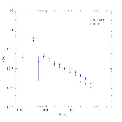
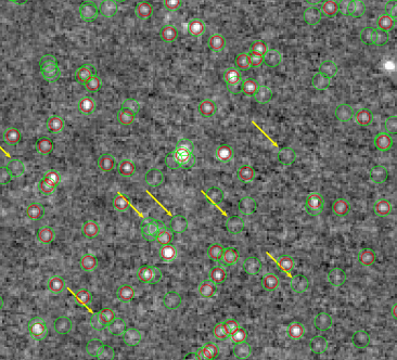
Figure 11.— Same as Figure 10 but the 2010-catalog sources are selected above a flux limit of $S_{24\,\mu\rm m}=180\,\mu$Jy. In the right panel, yellow arrows point to the faint sources in the 2010-catalog for which the flux measurements are significantly affected by the large-scale background variations.

Even though the A1-catalog appears to perform better for the smallest separations above its flux threshold, $S_{24\,\mu\rm m}=310\,\mu$Jy, the difference is rather small. The 2010-catalog, on the other hand, extends to significantly fainter fluxes, and so the question is, can we use these fainter sources to improve the statistics in the correlation function measurements? The comparison of the angular correlation function measurements in the Lockman Hole field for the A1- and 2010-catalogs above their respective flux limits of 310 and $180\,\mu$Jy is shown in Figure 11 (left). Unfortunately, there are systematic deviations for the 2010 sources at angular scales $0.2^{\circ}-0.5^{\circ}$ (recall that the results for the two catalogs were an excellent agreement for a common flux threshold of $310\,\mu$Jy, see Figure 10). The difference on these scales cannot be attributed to the edge effects—the size of the MIPS field in the Lockman Hole region is $\sim 4.6\times 1.9$ deg. Rather, we believe that this difference can be traced to how the large-scale structures in the MIPS background affect the flux measurements for fainter sources in the 2010-catalog. Examination of the MIPS image shows that, indeed, for a significant number of sources (some marked by yellow arrows in Figure 11 (right)), the flux above $180\,\mu$Jy is assigned spuriously, and many such sources appear on top of larger-scale background structures. These are likely real sources because by construction of the 2010-catalog, they have IRAC counterparts. It is also possible that these sources are suitable for measurements of the luminosity function or similar studies because an approximately equal number of objects “migrate” below $180\,\mu$Jy in those regions with the negative residual background. However, for clustering studies, these sources can not be used because they arise on top of spatially correlated structures and thus can distort the angular correlation function at intermediate scales.

As a final test, we compare the A1-based angular correlation functions for the Lockman Hole and ELAIS-S1 field (Figure 12). The limiting flux for the A1-catalog in the ELAIS-S1 field is $S_{24\,\mu\rm m}=400\,\mu$Jy. At all angular scales, the correlation function computed for sources above this threshold in the ELAIS-S1 field is in excellent agreement with that for the Lockman Hole field and $S_{24\,\mu\rm m}>310\,\mu$Jy.

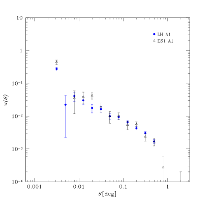
Figure 12.— Angular correlation function of $24\,\mu\rm m$ sources from A1- catalogs in Lockman Hole ($S_{24\,\mu\rm m}>310\,\mu$Jy) (blue filled circles) and ELAIS-S1 ($S_{24\,\mu\rm m}>400\,\mu$Jy) (black open triangles).

In summary, using our own, completely independent source detection algorithm we reproduced the $\log N$ – $\log S$ at $S_{24\,\mu\rm m}\gtrsim 300\mu$Jy and angular correlation function results at scales $\theta>0.01^{\circ}$ obtained for the 2010-catalog. The main analysis presented in this paper will lead to nearly identical results using either the 2010- or our A1-catalogs of the 24  $\mu\rm m$ sources. The most significant differences in the measured $w(\theta)$ are localized to $\theta<0.01^{\circ}$. They can be traced to different treatment of very crowded regions and zones in the immediate vicinity of bright sources, where our detection pipeline performs slightly better (Figure 10). On the basis of these considerations, we choose our A1-catalog in Lockman Hole to investigate clustering of $24\,\,\mu\rm m$ selected galaxies (Section 3).

References

- Amblard et al. (2011) Amblard, A., et al. 2011, Nature, 470, 510
- Berta et al. (2007) Berta, S., et al. 2007, A&A, 476, 151
- Berta et al. (2008) Berta, S., et al. 2008, A&A, 488, 533
- Bertin & Arnouts (1996) Bertin, E. & Arnouts, S. 1996, A&AS, 117, 393
- Blain et al. (2004) Blain, A. W., Chapman, S. C., Smail, I., & Ivison, R. 2004, ApJ, 611, 725
- Blain et al. (2002) Blain, A. W., Smail, I., Ivison, R. J., Kneib, J.-P., & Frayer, D. T. 2002, Phys. Rep., 369, 111
- Borgani & Kravtsov (2011) Borgani, S. & Kravtsov, A. 2011, Advanced Science Letters, 4, 204
- Bouwens et al. (2011) Bouwens, R. J., et al. 2011, ApJ, 737, 90
- Brand et al. (2009) Brand, K., et al. 2009, ApJ, 693, 340
- Brodwin et al. (2008) Brodwin, M., et al. 2008, ApJ, 687, L65
- Chary & Elbaz (2001) Chary, R. & Elbaz, D. 2001, ApJ, 556, 562
- Conroy et al. (2008) Conroy, C., Shapley, A. E., Tinker, J. L., Santos, M. R., & Lemson, G. 2008, ApJ, 679, 1192
- Conroy et al. (2006) Conroy, C., Wechsler, R. H., & Kravtsov, A. V. 2006, ApJ, 647, 201
- Cooray & Sheth (2002) Cooray, A. & Sheth, R. 2002, Phys. Rep., 372, 1
- Cooray et al. (2010) Cooray, A., et al. 2010, A&A, 518, L22+
- Daddi et al. (2007) Daddi, E., et al. 2007, ApJ, 670, 156
- Davé et al. (2010) Davé, R., Finlator, K., Oppenheimer, B. D., Fardal, M., Katz, N., Kereš, D., & Weinberg, D. H. 2010, MNRAS, 404, 1355
- de la Torre et al. (2007) de la Torre, S., et al. 2007, A&A, 475, 443
- de la Torre et al. (2010) de la Torre, S., et al. 2010, MNRAS, 409, 867
- Desai et al. (2008) Desai, V., et al. 2008, ApJ, 679, 1204
- Dey et al. (2008) Dey, A., et al. 2008, ApJ, 677, 943
- Dole et al. (2006) Dole, H., et al. 2006, A&A, 451, 417
- Elbaz et al. (2002) Elbaz, D., Cesarsky, C. J., Chanial, P., Aussel, H., Franceschini, A., Fadda, D., & Chary, R. R. 2002, A&A, 384, 848
- Fadda et al. (2010) Fadda, D., et al. 2010, ApJ, 719, 425
- Farrah et al. (2006) Farrah, D., et al. 2006, ApJ, 641, L17
- Farrah et al. (2008) Farrah, D., et al. 2008, ApJ, 677, 957
- Fazio et al. (2004) Fazio, G. G., et al. 2004, ApJS, 154, 10
- Fiolet et al. (2009) Fiolet, N., et al. 2009, A&A, 508, 117
- Fiolet et al. (2010) Fiolet, N., et al. 2010, A&A, 524, A33
- Franceschini et al. (2010) Franceschini, A., Rodighiero, G., Vaccari, M., Berta, S., Marchetti, L., & Mainetti, G. 2010, A&A, 517, A74+
- Franceschini et al. (2005) Franceschini, A., et al. 2005, AJ, 129, 2074
- Genzel & Cesarsky (2000) Genzel, R. & Cesarsky, C. J. 2000, ARA&A, 38, 761
- Gilli et al. (2007) Gilli, R., et al. 2007, A&A, 475, 83
- González-Solares et al. (2011) González-Solares, E. A., et al. 2011, MNRAS, 416, 927
- Granato et al. (2004) Granato, G. L., De Zotti, G., Silva, L., Bressan, A., & Danese, L. 2004, ApJ, 600, 580
- Grazian et al. (2006) Grazian, A., et al. 2006, A&A, 449, 951
- Guo et al. (2010) Guo, Q., White, S., Li, C., & Boylan-Kolchin, M. 2010, MNRAS, 404, 1111
- Hauser & Dwek (2001) Hauser, M. G. & Dwek, E. 2001, ARA&A, 39, 249
- Hauser et al. (1998) Hauser, M. G., et al. 1998, ApJ, 508, 25
- Hopkins (2004) Hopkins, A. M. 2004, ApJ, 615, 209
- Huang et al. (2009) Huang, J., et al. 2009, ApJ, 700, 183
- Ilbert et al. (2009) Ilbert, O., et al. 2009, ApJ, 690, 1236
- Klypin & Holtzman (1997) Klypin, A. & Holtzman, J. 1997, ArXiv:astro-ph/9712217
- Klypin et al. (2011) Klypin, A. A., Trujillo-Gomez, S., & Primack, J. 2011, ApJ, 740, 102
- Komatsu et al. (2009) Komatsu, E., et al. 2009, ApJS, 180, 330
- Komatsu et al. (2011) Komatsu, E., et al. 2011, ApJS, 192, 18
- Kravtsov et al. (2004) Kravtsov, A. V., Berlind, A. A., Wechsler, R. H., Klypin, A. A., Gottlöber, S., Allgood, B., & Primack, J. R. 2004, ApJ, 609, 35
- Kravtsov & Klypin (1999) Kravtsov, A. V. & Klypin, A. A. 1999, ApJ, 520, 437
- Lacey et al. (2010) Lacey, C. G., Baugh, C. M., Frenk, C. S., Benson, A. J., Orsi, A., Silva, L., Granato, G. L., & Bressan, A. 2010, MNRAS, 405, 2
- Lagache et al. (2005) Lagache, G., Puget, J., & Dole, H. 2005, ARA&A, 43, 727
- Landy & Szalay (1993) Landy, S. D. & Szalay, A. S. 1993, ApJ, 412, 64
- Le Floc’h et al. (2005) Le Floc’h, E., et al. 2005, ApJ, 632, 169
- Le Floc’h et al. (2009) Le Floc’h, E., et al. 2009, ApJ, 703, 222
- Lee et al. (2006) Lee, K., Giavalisco, M., Gnedin, O. Y., Somerville, R. S., Ferguson, H. C., Dickinson, M., & Ouchi, M. 2006, ApJ, 642, 63
- Limber (1953) Limber, D. N. 1953, ApJ, 117, 134
- Lonsdale et al. (2003) Lonsdale, C. J., et al. 2003, PASP, 115, 897
- Lonsdale et al. (2009) Lonsdale, C. J., et al. 2009, ApJ, 692, 422
- Madau et al. (1996) Madau, P., Ferguson, H. C., Dickinson, M. E., Giavalisco, M., Steidel, C. C., & Fruchter, A. 1996, MNRAS, 283, 1388
- Maddox et al. (2010) Maddox, S. J., et al. 2010, A&A, 518, L11+
- Magliocchetti et al. (2007) Magliocchetti, M., Silva, L., Lapi, A., de Zotti, G., Granato, G. L., Fadda, D., & Danese, L. 2007, MNRAS, 375, 1121
- Magliocchetti et al. (2008) Magliocchetti, M., et al. 2008, MNRAS, 383, 1131
- Makovoz & Marleau (2005) Makovoz, D. & Marleau, F. R. 2005, PASP, 117, 1113
- Myers et al. (2005) Myers, A. D., Outram, P. J., Shanks, T., Boyle, B. J., Croom, S. M., Loaring, N. S., Miller, L., & Smith, R. J. 2005, MNRAS, 359, 741
- Nagai & Kravtsov (2005) Nagai, D. & Kravtsov, A. V. 2005, ApJ, 618, 557
- Narayanan et al. (2010) Narayanan, D., et al. 2010, MNRAS, 407, 1701
- Peebles (1980) Peebles, P., The Large Scale Structure of the Universe (Princeton University Press, 1980)
- Peebles (1974) Peebles, P. J. E. 1974, A&A, 32, 197
- Polletta et al. (2007) Polletta, M., et al. 2007, ApJ, 663, 81
- Porciani & Giavalisco (2002) Porciani, C. & Giavalisco, M. 2002, ApJ, 565, 24
- Puget et al. (1996) Puget, J., Abergel, A., Bernard, J., Boulanger, F., Burton, W. B., Desert, F., & Hartmann, D. 1996, A&A, 308, L5+
- Quadri et al. (2007) Quadri, R., et al. 2007, ApJ, 654, 138
- Quadri et al. (2008) Quadri, R. F., Williams, R. J., Lee, K., Franx, M., van Dokkum, P., & Brammer, G. B. 2008, ApJ, 685, L1
- Revnivtsev et al. (2007) Revnivtsev, M., Vikhlinin, A., & Sazonov, S. 2007, A&A, 473, 857
- Rieke et al. (2004) Rieke, G. H., et al. 2004, ApJS, 154, 25
- Rigby et al. (2004) Rigby, J. R., et al. 2004, ApJS, 154, 160
- Roche et al. (1993) Roche, N., Shanks, T., Metcalfe, N., & Fong, R. 1993, MNRAS, 263, 360
- Rodighiero et al. (2010) Rodighiero, G., et al. 2010, A&A, 515, A8+
- Ross et al. (2007) Ross, N. P., et al. 2007, MNRAS, 381, 573
- Rowan-Robinson et al. (2008) Rowan-Robinson, M., et al. 2008, MNRAS, 386, 697
- Sacchi et al. (2009) Sacchi, N., et al. 2009, ApJ, 703, 1778
- Sanders & Mirabel (1996) Sanders, D. B. & Mirabel, I. F. 1996, ARA&A, 34, 749
- Sanders et al. (2007) Sanders, D. B., et al. 2007, ApJS, 172, 86
- Santini et al. (2009) Santini, P., et al. 2009, A&A, 504, 751
- Scott et al. (2006) Scott, S. E., Dunlop, J. S., & Serjeant, S. 2006, MNRAS, 370, 1057
- Scranton et al. (2002) Scranton, R., et al. 2002, ApJ, 579, 48
- Shupe et al. (2008) Shupe, D. L., et al. 2008, AJ, 135, 1050
- Silverman et al. (2005) Silverman, J. D., et al. 2005, ApJ, 624, 630
- Skrutskie et al. (2006) Skrutskie, M. F., et al. 2006, AJ, 131, 1163
- Soifer et al. (2008) Soifer, B. T., Helou, G., & Werner, M. 2008, ARA&A, 46, 201
- Springel et al. (2005) Springel, V., et al. 2005, Nature, 435, 629
- Surace et al. (2005) Surace, J. A., Shupe, D. L., Fang, F., Evans, T., Alexov, A., Frayer, D., Lonsdale, C. J., & SWIRE Team 2005, BAAS, 37, 1246
- Treister et al. (2006) Treister, E., et al. 2006, ApJ, 640, 603
- Viero et al. (2009) Viero, M. P., et al. 2009, ApJ, 707, 1766
- Vikhlinin et al. (1995) Vikhlinin, A., Forman, W., Jones, C., & Murray, S. 1995, ApJ, 451, 553
- Vikhlinin et al. (1998) Vikhlinin, A., McNamara, B. R., Forman, W., Jones, C., Quintana, H., & Hornstrup, A. 1998, ApJ, 502, 558
- Vikhlinin et al. (2009) Vikhlinin, A., et al. 2009, ApJ, 692, 1060
- Waddington et al. (2007) Waddington, I., et al. 2007, MNRAS, 381, 1437
- Weiß et al. (2009) Weiß, A., et al. 2009, ApJ, 707, 1201
- Werner et al. (2004) Werner, M. W., et al. 2004, ApJS, 154, 1
- Yan et al. (2005) Yan, L., et al. 2005, ApJ, 628, 604
- Zehavi et al. (2002) Zehavi, I., et al. 2002, ApJ, 571, 172