Fluctuation Relations for Spintronics

Abstract

Fluctuation relations are derived in systems where the spin degree of freedom and magnetic interactions play a crucial role. The form of the non-equilibrium fluctuation theorems relies in the assumption of a local balance condition. We demonstrate that in some cases the presence of magnetic interactions violates this condition. Nevertheless, fluctuation relations can be obtained from the micro-reversibility principle sustained only at equilibrium as a symmetry of the cumulant generating function for spin currents. We illustrate the spintronic fluctuation relations for a quantum dot coupled to partially polarized helical edges states .

Introduction.

Non-equilibrium fluctuation theorems (FTs) PhysRevLett.78.2690 ; PhysRevE.60.2721 ; RevModPhys.81.1665 , widely used for macroscopic systems, are based on the thermodynamics governing the physical processes when they evolve forward and backward in time. The boundary conditions for the forward and the time-reversed processes determine the balance condition for the entropy exchange and therefore the form of the fluctuation theorem RevModPhys.81.1665 . The applicability of the non-equilibrium FTs to quantum systems has become an exciting problem and, in particular, to the case of the charge transfer phenomena in mesoscopic systems in the context of the full counting statistics levitov ; PhysRevLett.88.196801 ; PhysRevLett.90.206801 ; 1742-5468-2006-01-P01011 . Interestingly, relations akin to the fluctuation-dissipation theorem PhysRev.32.110 ; PhysRev.32.97 ; JPSJ.12.570 ; Einstein.1905 have been formulated beyond the linear response regime PhysRevB.72.235328 ; 1742-5468-2006-01-P01011 ; PhysRevLett.101.046802 ; PhysRevB.78.115429 ; PhysRevLett.101.136805 ; san09 ; san10 ; lim10 ; gol11 ; bul11 ; kra11 ; gan11 . These fluctuation relations relate nonequilibrium fluctuation and dissipation coefficients for phase-coherent conductors. However, the role of a genuine quantum property such as the spin degree of freedom in the fluctuation relations has not been yet investigated in detail. Our motivation is not only fundamental since the electronic spin offers enormous advantages to create devices with unusual and extraordinary new functionalities fab07 . The purpose of this work is thus to generalize the fluctuation relations for spintronic systems.

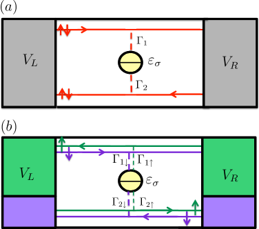
Figure 1: (Color online) (a) Sketch of a quasi-localized level ($\varepsilon_{\sigma}$) coupled to chiral edge states with $\Gamma_{1,2}$ and driven out of equilibrium with $V_{L}$ and $V_{R}$ bias voltages. For $B>0$ the upper (lower) edge state is injected from $V_{L}$ ($V_{R}$). (b) Localized level coupled to unequally spin populated helical edge states due to the spin injection from the ferromagnetic leads. Then, the tunnelling couplings are spin-dependent: $\Gamma_{(1,2)\uparrow(\downarrow)}$. Ferromagnetic electrodes: larger light area (green) corresponds to majority spins whereas smaller dark area (purple) are minority spins. Helical states: upper left (upper right) movers are spin up (spin down) carriers injected from $V_{R}$ ($V_{L}$).

Fluctuation relations are generated from the cumulant generating function (CGF) $\mathcal{F}(\chi)=\ln\sum_{Q}P(Q,t)e^{-i\chi Q}$ where $P(Q)$ is the charge distribution function. Firstly, the CGF $\mathcal{F}$ is expanded in a Taylor expansion in terms of affinities $A=\left(qV_{1}/k_{B}T,qV_{2}/k_{B}T,\cdots\right)$ ($q$ is the electron charge, $k_{B}$ is the Boltzmann constant, $T$ is the temperature and $V_{i}$, $i=1,2\dots$ are the applied voltages) and counting fields $\chi=\left(\chi_{1},\chi_{2},\cdots\right)$ around the equilibrium condition. Then, thanks to the symmetries $F(0,A)=0$ (probability conservation condition) and $F(-A,A)=0$ (global detailed balance condition) fluctuation relations among the higher-order non-linear cumulants are found. Indeed, the symmetries of $\mathcal{F}$ can be considered as the non-equilibrium FT versions for the currents within a transport theory. Initial experiments by using a mesoscopic dot interferometer have tested these relations PhysRevLett.104.080602 . In this experiment, the noise susceptibility and the second order conductance were found to be proportionally related.

Spins are sensitive to magnetic fields and also to electric fields due to spin-orbit interactions. Fluctuation relations for the charge transport have been formulated in the presence of magnetic fields PhysRevB.78.115429 ; PhysRevLett.101.136805 ; san09 . In Ref. PhysRevB.78.115429 the non-equilibrium FT for the forward and backward charge distribution probability at opposite $B$ polarities $P(Q,B)/P(-Q,-B)=e^{QA}$ was used to derive such fluctuation relations. However, some caution is needed since $P(Q,B)$ and $P(-Q,-B)$ are considered for a system driven out of equilibrium in which the interacting internal potentials are no longer even functions of $B$ Sánchez and Büttiker (2004) and the application of such theorem may break down PhysRevLett.101.136805 . To circumvent this obstacle, Ref. PhysRevLett.101.136805 uses a symmetry of $\mathcal{F}$ associated with the micro-reversibility condition only at equilibrium $P(Q,B)_{A\to 0}=P(-Q,-B)_{A\to 0}$. We here derive the spintronic fluctuation relations in the same spirit when time-reversal symmetry is broken not only by external magnetic fields but also by the presence of ferromagnetic electrodes. In this case, at equilibrium $P(Q,B,p)_{A\to 0}=P(Q,-B,-p)_{A\to 0}$, where $p$ is the lead magnetization ada06 .

We illustrate our findings with a quasi-localized level coupled to helical edge states which are partially polarized by the presence of polarized electrodes [see Fig. 1 (b)]. Helical modes have been observed in topological insulators Hasan and Kane (2010) and proposed to occur in quantum wires Kloeffel et al. (2011) and in carbon nanotubes Klinovaja et al. (2011). This quantum spin Hall state consists of gapless excitations that exist at the boundaries in which its propagation direction is correlated with its spin due to the spin-orbit interaction. By electrostatic gating, quasi-localized states can form in the interior of the carbon nanotubes and quantum wires. Furthermore, ferromagnetic contacts have been successfully attached to these nanodevices Tsukagoshi et al. (2011). Finally, Ref. Carsten (2011) suggests to create a quasi-bound state in quantum spin Hall setups by using ferromagnetic insulators that serve as tunnelling barriers.

Local Detailed Balance.

Consider a system described by a set of $m$ discrete states coupled to $\ell$-electronic reservoirs. We assume that its dynamics is governed by the master equation $d\rho/dt=\mathcal{W}\rho$, where $\mathcal{W}$ is the transition rate matrix, and $\rho$ denotes the occupation probabilities for the $m$-states. The exchange of energy ($\Delta E^{(\ell)}$) or particles ($\Delta N^{(\ell)}$) in the $\ell$-th-reservoir with inverse temperature $\beta^{(\ell)}$ is described by adding counting fields ($\chi_{E}^{(\ell)}$, $\chi_{N}^{(\ell)}$) to the off-diagonal matrix elements of $\mathcal{W}$. Thus, for the upper off-diagonal the transition rate from the state $n$ to the state $m$ are modified according to $W_{nm}=\sum_{\ell}W^{(\ell)}_{nm}e^{\chi_{E}^{(\ell)}\Delta E^{(\ell)}+\chi_{N}^{(\ell)}\Delta N^{(\ell)}}$ (for $n<m$) whereas for the lower off-diagonal terms these rates are $W_{nm}=\sum_{\ell}W^{(\ell)}_{nm}e^{-\chi_{E}^{(\ell)}\Delta E^{(\ell)}-\chi_{N}^{(\ell)}\Delta N^{(\ell)}}$ ($n>m$). Usually, boundary conditions are taken into account through the local detailed balance (LDB) condition in which weight factors $e^{-\beta^{(\ell)}(\mathcal{H_{\ell}}-\mu N_{\ell})}$ ($\mathcal{H_{\ell}}$, and $N_{\ell}$ denote the Hamiltonian and the particle number operator, respectively for the $\ell$th-reservoir) balance forward and backward processes. To be more specific:

$$\frac{W^{(\ell)}_{nm}}{W^{(\ell)}_{mn}}=e^{-\beta^{(\ell)}(\Delta E^{(\ell)}-\mu^{(\ell)}\Delta N^{(\ell)})}\,.$$ (1)

From the LDB condition the equality $\mathcal{W}(\chi_{E}^{(\ell)},\chi_{N}^{(\ell)})=\mathcal{W}^{T}(\beta^{(\ell)}-\chi_{E}^{(\ell)},-\beta^{(\ell)}\mu^{(\ell)}-\chi_{N}^{(\ell)})$ is automatically satisfied reflecting the following symmetry for the generating function $\mathcal{F}$ [which is constructed from $\mathcal{W}(\chi_{E}^{(\ell)},\chi_{N}^{(\ell)}$)]:

$$\mathcal{F}[\chi_{E}^{(\ell)},\chi_{N}^{(\ell)})]=\mathcal{F}[\beta^{(\ell)}-\chi_{E}^{(\ell)},-\beta^{(\ell)}\mu^{(\ell)}-\chi_{N}^{(\ell)}]\,.$$ (2)

Although in many systems we can assume some type of LDB condition, in general, Eq.(1) is not fulfilled vai2007 . To see this in a quantum conductor, we consider the system sketched in Fig. 1(a) in which the presence of a magnetic field breaks time-reversal symmetry. The system consists of a quasi-localized state with energy $\varepsilon_{d}$ in the Coulomb blockade regime coupled to two chiral states propagating along the opposite edges of a quantum Hall conductor (filling factor $\nu=1$) Sánchez and Büttiker (2004); san09 ; wang2011 . In the infinite charging energy limit case only two dot charge states are permitted: $|0\rangle$ and $|1\rangle$. For positive magnetic fields $B>0$ carriers in the upper (lower) edge state move from the left (right) terminal to the right (left) terminal. The current flow is reversed for $B<0$. Interaction between the quasi-localized state and the edge states takes place via tunnel couplings $\Gamma_{1}$ and $\Gamma_{2}$ and capacitive couplings $C_{1}$ and $C_{2}$. The chiral coupling involves different transition rates depending on the polarity of the magnetic field. For a positive $B$ we have $W_{01}^{L(R)}=\Gamma_{1(2)}f(B,\mu_{L(R)})$, $W_{10}^{L(R)}=\Gamma_{1(2)}[1-f(B,\mu_{L(R)})]$, where $f(B,\mu_{L(R)})=1/(1+\exp{\beta[\mu_{d}(B)-\mu_{L(R)}]})$ is the Fermi-Dirac distribution function, $\mu_{L(R)}=qV_{L(R)}+E_{F}$ denotes the electrochemical potential in the lead $L(R)$ with $E_{F}=0$ the Fermi energy, and $\mu_{d}$ is the electrochemical potential of the quasi-localized state which is self-consistently calculated and depends on the $B$ orientation san09 . For $B>0$, $\mu_{d}(B)-\mu_{L}=\varepsilon_{d}-(1-\eta)qV/2$, where $\eta=(C_{1}-C_{2})/(C_{1}+C_{2})$ is the capacitance asymmetry parameter and $V=V_{L}-V_{R}$. For $B<0$ the motion of the edge states is reversed and then $\mu_{d}(-B)-\mu_{L}=\varepsilon_{d}-(1+\eta)qV/2$. Because of the fact that $\mu_{d}(B)\neq\mu_{d}(-B)$, the LDB condition is not satisfied. Clearly,

$$\frac{W^{L}_{10}(B)}{W^{L}_{01}(-B)}=e^{\beta(\varepsilon_{d}-qV/2)}[1-\beta\eta\frac{qV}{2}\tilde{f}_{eq}+\mathcal{O}(V^{2})]\,,$$ (3)

where $\beta$ is the common inverse temperature and $\tilde{f}_{eq}=1-2f_{eq}$ with $f_{eq}$ being the Fermi function at equilibrium ($V_{L}=V_{R}$) . Importantly, the violation of the LDB condition occurs for asymmetric capacitance couplings only. In the symmetric case or at equilibrium, Eq. (1) is recovered. The violations of LDB are thus a consequence of asymmetric, chiral states out of equilirium

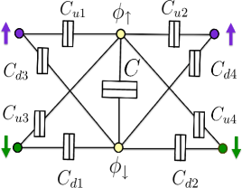
Figure 2: (Color online) Electrostatic model for the quasi-localized state connected to helical spin edge states. Spin up(down) localized level is capacitatively coupled to the upper up(down) helical channel with capacitances $C_{u1(u3)}[C_{d1(d3)}]$ and to the lower up(down) helical channel with capacitances $C_{u2(u4)}[C_{d2(d4)}]$. A mutual capacitance between up and down localized levels is accounted for with $C$. $\phi_{\uparrow(\downarrow)}$ denotes the spin up (down) internal potential for the quasi-bound state.

We now show that violations of the LDB conditions are also present in the absence of magnetic fields and when the spin degree of freedom is explicitly accounted for. For that purpose we consider the system sketched in Fig. 1(b), a quasi-bound state which is tunnel coupled to helical edge states. The helical modes are partially polarized due to their coupling to two ferromagnetic electrodes with parallel magnetization and equal polarization $p$. In this manner, polarized helical edge states are described with a spin-dependent density of states (DOS) $D_{is}=(1+sp)D_{i}/2$, where $s=+(-)$ for $\uparrow(\downarrow)$-helical mode and, $D_{i}$, with $i=u,d$ denoting the upper and lower edge-state DOS in the absence of polarization Christen and Büttiker (1996). In the wide band limit approximation, the tunnelling rates become spin-dependent, $\Gamma_{is}=\pi|t_{i}|^{2}D_{is}$, with $|t_{i}|^{2}$ the tunnel probability from the $i$-th edge state. Defining $\Gamma_{i}=\pi|t_{i}|^{2}D_{i}$, we find $\Gamma_{is}=(1+sp)\Gamma_{i}/2$.

Our transport description also includes an electrostatic model for interactions between the dot and the edge states. Within the mean-field approach, the electrochemical capacitive coupling $C_{\mu}$ consists of a geometrical capacitance contribution, $C_{g}$, which depends on the width and the height of the tunnel barrier, and a quantum capacitance term, $C_{is,q}$, which we take as proportional to $D_{is}$:

$$C_{\mu is}^{-1}=\frac{1}{C_{g}}+\frac{1}{q^{2}D_{is}}\,.$$ (4)

We emphasize that the capacitive couplings are, in general, spin dependent mac99 . For sufficiently large geometrical capacitances, $C_{g}\gg C_{is,q}$, we find from Eq. (4) the capacitative couplings

$$C_{u1(2)}=\frac{1+p}{2}C_{1(2)},\,\,C_{u3(4)}=\frac{1-p}{2}C_{3(4)}\,,$$ (5)

where $C_{i}=q^{2}D_{i}$ with $C_{u1(d1)}$, $C_{u2(d2)}$ being the capacitive couplings between left (right) movers with up (down) spin along the top edge and the dot electron with spin $\uparrow$ ($\downarrow$) whereas $C_{u3(d3)}$ and $C_{u4(d4)}$ couple the same dot state with right (left) movers along the bottom edge with up (down) spins (see Fig. 2). For thin edge states, $D_{i}$ depends on the steep confinement potential at the top and bottom edges, which will generally differ Christen and Büttiker (1996). Then, we take $C_{1}=C_{3}$ and $C_{2}=C_{4}$ but $C_{1}\neq C_{2}$. As a consequence, the capacitive couplings between the dot and the edges is asymmetric: $\eta\neq 0$. Furthermore, since the upper and lower edge modes are equally polarized, one has $C_{dj}=C_{uj}$.

Consider for the moment the case where the capacitance coupling between the dot states is neglected ($C=0$). Then, we calculate the spin-dependent electrochemical potential of the dot and find the simple relation $\mu_{\sigma}(p)-\mu_{\bar{\sigma}}(-p)=p\eta V$. Now, in a time-reversal operation we have to invert the lead polarization, the edge state spin index, and the dot spin. Doing so, we obtain an invariant result only at equilibrium ($V=0$) or for symmetric capacitive couplings. But, in general, when $V\neq 0$ the original state is not restored and, as a consequence, LDB is not fulfilled:

$$\frac{W_{0\sigma}(p)}{W_{\bar{\sigma}0}(-p)}=e^{\beta[\varepsilon_{d}-qV/2]}[1-\beta\eta p\frac{qV}{2}\tilde{f}_{eq}+\mathcal{O}(V^{2})],$$ (6)

where $\sigma=\{\uparrow,\downarrow\}$ denotes the dot spin index. We stress that helicity is needed in our example to find departures from LDB. Although we cannot rule out the possibility that nonchiral, spintronic systems (e.g., a dot directly attached to ferromagnetic leads) might show such departures if coherent tunneling or strong correlations are taken into accoutn, our conceptually simple system already exhibits the effect with fully analytical expressions.

Spintronic fluctuation relations.

We now treat on equal footing the presence of both magnetic fields and polarized contacts. The spin-dependent probability distribution satisfies the micro-reversibility condition, but only at equilibrium

$$P(\{n_{\alpha{s}},n_{\beta{s^{\prime}}},\ldots\};B,p)\\ =P(\{-n_{\alpha{\bar{s}}},-n_{\beta{\bar{s^{\prime}}}},\ldots\};-B,-p)\,,$$ (7)

where $\alpha$ and $s$ are the lead and spin indices, respectively and $p\equiv(p,p^{\prime},\cdots)$ contains the magnetizations for the leads. The CGF $\mathcal{F}(\{i\chi\},A)$ can be expanded in terms of powers of voltages and counting fields

$$\mathcal{F}(\{i\chi\},A)=\sum_{\{k_{\alpha s}\},\{l_{\alpha}\}}f_{\{k_{\alpha s}\},\{l_{\alpha}\}}\frac{\prod_{\alpha s}(i\chi_{\alpha s})^{k_{\alpha s}}\prod_{\alpha}A_{\alpha}^{l_{\alpha}}}{\prod_{\alpha}k_{\alpha s}!\prod_{\alpha}l_{\alpha}!}$$ (8)

and

$$f_{\{k_{\alpha s}\},\{l_{\alpha}\}}=\prod_{\alpha s}\partial^{k_{\alpha s}+l_{\alpha}}\mathcal{F}(\{i\chi\},A)/\partial(i\chi_{\alpha s})^{k_{\alpha s}}\partial A_{\alpha}^{l_{\alpha}}\Big{|}_{i\chi\to 0,A\to 0}$$ (9)

where $k$ and $l$ are non-negative integers. From the derivatives of $\mathcal{F}(\{i\chi\},A)$ with respect to the counting fields, the cumulants are generated. In this way, the average current through terminal $\alpha$ with spin $s$ is derived from Eq. (8) as $\langle I_{\alpha s}\rangle=f_{\{1_{\alpha s}\}}$. Similarly, second cumulant (current-current correlation) $S_{\alpha s,\beta s^{\prime}}\equiv\langle\Delta I_{\alpha s}\Delta I_{\beta s^{\prime}}\rangle$ ($\Delta I_{\alpha s}=\hat{I}_{\alpha s}-\langle I_{\alpha s}\rangle)$, where $\hat{I}$ denotes the current operator) and the third cummulant $C_{\alpha s\beta s^{\prime}\gamma s^{\prime\prime}}\equiv\langle\Delta I_{\alpha s}\Delta I_{\beta s^{\prime}}\Delta I_{\gamma s^{\prime\prime}}\rangle$ are given by $S_{\alpha s\beta s^{\prime}}=f_{\{1_{\alpha s}1_{\beta s^{\prime}}\}}$ and $C_{\alpha s\beta s^{\prime}\gamma s^{\prime\prime}}=f_{\{1_{\alpha s}1_{\beta s^{\prime}}1_{\gamma s^{\prime\prime}}\}}$, respectively. We expand, both, the current $\langle I_{\alpha s}\rangle$, and the noise $\langle S_{\alpha s\beta s^{\prime}}\rangle$ in powers of the applied voltages as follows

$$\langle I_{\alpha s}\rangle=\sum_{j}G_{\alpha s,j}^{(1)}V_{j}+\frac{1}{2}\sum_{j,k}G_{\alpha s,jk}^{(2)}V_{j}V_{k}+\mathcal{O}(V^{3})\,,$$

$$\langle S_{\alpha s\beta s^{\prime}}\rangle=S_{\alpha s\beta s^{\prime}}^{(0)}+\sum_{j}S_{\alpha s\beta s^{\prime},j}^{(1)}V_{j}+\mathcal{O}(V^{2})\,.$$ (10)

Here $G_{\alpha s,j}^{(1)}=f_{\{1_{\alpha s}\},\{1_{j}\}}$ corresponds to the linear conductance, $G_{\alpha s,jk}^{(2)}=f_{\{1_{\alpha s}\},\{1_{j}1_{k}\}}$ is the second-order conductance, and $S_{\alpha s,\beta s^{\prime},j}^{(1)}=f_{\{1_{\alpha s}1_{\beta s^{\prime}}\},\{1_{j}}\}$ is the noise susceptibility. Fluctuation relations are expressions that relate the $f$-coefficients at different order in voltage. To derive explicitly these relations we employ the micro-reversibility condition at equilibrium $F(i\chi_{\alpha s},i\chi_{\beta s^{\prime}},\cdots,A,+B)|_{A=0}=F(-i\chi_{\alpha\bar{s}},-i\chi_{\beta\bar{s^{\prime}}},\cdots,A,-B)|_{A=0}$ [cf. Eq. (7)]. It is convenient to define the symmetrized ($+$) and anti-symmetrized ($-$) combination of the $f$-factors

$$f_{\{k_{\alpha s}\},\{l_{j}\}}^{\pm}=f_{\{k_{\alpha s}\},\{l_{j}\}}(B,p)\pm f_{\{k_{\alpha\bar{s}}\},\{l_{j}\}}(-B,-p)\,.$$ (11)

where $f_{\{k_{\alpha\bar{s}}\},\{l_{j}\}}(-B,-p)$ is generated by means of time reversal operation $B\to-B$, $p\to-p$, and $s\to-s$. According to Eq. (7) the $f^{\pm}$-factors are even(odd) functions under time-reversal operation. This even-odd property is translated into the following relations for the equilibrium coefficients [in the sense of a voltage expansion, see Eqs. (Spintronic fluctuation relations.)]:

$$S_{\alpha s\beta s^{\prime}}^{(0)}(B,p)=S_{\alpha\bar{s}\beta\bar{s}^{\prime}}^{(0)}(-B,-p)\,,$$ (12)

$$C_{\alpha s\beta s^{\prime}\gamma s^{\prime\prime}}^{(0)}(B,p)=-C_{\alpha\bar{s}\beta\bar{s}^{\prime}\gamma\bar{s}^{\prime\prime}}^{(0)}(-B,-p)\,.$$

Now by using the global detailed balance condition $\mathcal{F}(-A,A)_{\pm}=0$, and the probability conservation $\mathcal{F}(0,A)_{\pm}=0$ one can derive the spintronic fluctuation relations among different $f_{\pm}$-factors. Here we explicitly show those that relate the coefficients appearing in the third cumulant, noise and the conductances in the voltage expansion of Eq. (Spintronic fluctuation relations.):

$$C_{\alpha s\beta s^{\prime}\gamma s^{\prime\prime}\pm}^{(0)}$$

$$= k_{B}T\Big{[}S^{(1)}_{\alpha s\beta s^{\prime},\gamma\pm}+S^{(1)}_{\alpha s\gamma s^{\prime\prime},\beta\pm}+S^{(1)}_{\beta s^{\prime}\gamma s^{\prime\prime},\alpha\pm}$$

$$- k_{B}T\left(G^{(2)}_{\alpha s,\beta\gamma\pm}+G^{(2)}_{\beta s^{\prime},\alpha\gamma\pm}+G^{(2)}_{\gamma s^{\prime\prime},\alpha\beta\pm}\right)\Big{]}\,.$$

Fluctuation relations between even higher-order response coefficients toward the strongly nonequilibrium domain can be similarly found, relating different current cumulants at different order; however, the resulting expressions, already in the spinless case, look rather cumbersome PhysRevLett.101.136805 .

We verify Eq. (Spintronic fluctuation relations.) in a multi-terminal setup in which LDB condition is broken. For that purpose we generalize the two terminal quantum spin Hall bar system [Fig. 1(b)] to the multi-terminal case in which upper and lower helical modes are now connected to different terminals $V_{i}$, $i=1\cdots 4$ [see inset in Fig. 3(d)]. We additionally consider spin-flip relaxation events within the quasi-bound state that can occur due to spin-spin interactions with a spin fluctuating environment (hyperfine interaction, spin-orbit interactions, etc.). We phenomenologically model this rate as $\gamma_{sf}^{\sigma\bar{\sigma}}=\gamma_{sf}\exp\left[(\varepsilon_{\sigma}-\varepsilon_{\bar{\sigma}})/(2k_{B}T)\right]$. Notice that due to spin-flip events spin up and down currents are correlated and then Eq. (Spintronic fluctuation relations.) is satisfied in a non-trivial manner. We emphasize that Eq. (Spintronic fluctuation relations.) is verified (see Fig. 3) even for a finite capacitance asymmetry where the LDB condition is not met.

Conclusions.

In short, we have shown that the applicability of non-equilibrium FT when magnetic interactions are present is not a priori ensured. We illustrate this statement by using a quasi-localized level coupled to a chiral one-dimensional conducting channels. We demonstrate that local detailed balance condition is not satisfied when a magnetic field is included and the system is driven out of equilibrium. Importantly, we have derived the fluctuation relations for spintronic systems and have explicitly verified them in the illustrative case of a quasi-localized state coupled to partially polarized helical edge states. Our formalism is based on zero-frequency fluctuations and time-independent fields but in the presence of arbitrary interactions. Promising avenues for future work include finite-frequency calculations and ac fields.

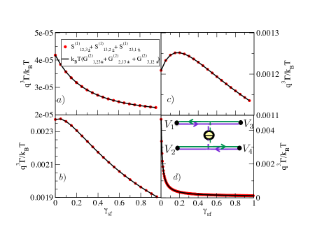
Figure 3: Verification of spintronic fluctuation relations as a function of $\gamma_{sf}$ in the presence of magnetic interactions, $B$, and $p$ for different values of polarization $p$: (a) $p=0$, (b) $p=0.25$, (c) $p=0.5$, and (d) $p=0.75$. Upper helical modes: left (right) movers are spin up (down) injected with voltage $V_{1(3)}$. Lower helical modes: right (left) movers are spin up (down) injected with voltage $V_{2(4)}$. Parameters: $\Gamma=1$, $q^{2}/[4(C_{1}+C_{2})]=40\Gamma$, $\varepsilon_{d}=0$, $k_{B}T=5\Gamma$, $g\mu_{B}B=0.1\Gamma$ and capacitance asymmetry $\eta=0.5$. Note that in our chiral system spin indices are included in the lead indices for the fluctuation relations.

References

- (1) C. Jarzynski, Phys. Rev. Lett. 78, 2690 (1997).
- (2) G. E. Crooks, Phys. Rev. E 60, 2721 (1999).
- (3) M. Esposito, U. Harbola, and S. Mukamel, Rev. Mod. Phys. 81, 1665 (2009).
- (4) L. S. Levitov and G. B. Lesovik, Pis’ma Zh. Eksp. Teor. Fiz. 58, 225 (1993).
- (5) Y. V. Nazarov and D. A. Bagrets, Phys. Rev. Lett. 88, 196801 (2002).
- (6) S. Pilgram, A. N. Jordan, E. V. Sukhorukov, and M. Büttiker, Phys. Rev. Lett. 90, 206801 (2003).
- (7) D. Andrieux and P. Gaspard, J. Stat. Mech. P01011 (2006).
- (8) H. Nyquist, Phys. Rev. 32, 110 (1928).
- (9) J. B. Johnson, Phys. Rev. 32, 97 (1928).
- (10) R. Kubo, J. Phys. Soc. Jpn. 12, 570 (1957).
- (11) A. Einstein, Ann. Phys. Lpz. 322, 549 (1905).
- (12) J. Tobiska and Y. V. Nazarov, Phys. Rev. B 72, 235328 (2005).
- (13) R. D. Astumian, Phys. Rev. Lett. 101, 046802 (2008).
- (14) K. Saito and Y. Utsumi, Phys. Rev. B 78, 115429 (2008); Phys. Rev. B 79, 235311 (2009); J. Phys. Conf. Series 200, 052030 (2010).
- (15) H. Förster and M. Büttiker, Phys. Rev. Lett. 101, 136805 (2008); AIP Conf. Proc. 1129, 443 (2009).
- (16) D. Sánchez, Phys. Rev. B 79, 045305 (2009).
- (17) R. Sánchez, R. López, D. Sánchez, and M. Büttiker, Phys. Rev. Lett. 104, 076801 (2010).
- (18) J.S. Lim, D. Sánchez, and R. López, Phys. Rev. B 81, 155323 (2010); AIP Conf. Proc. 1129, 435 (2009).
- (19) D. S. Golubev, Y. Utsumi, M. Marthaler, and G. Schön, Phys. Rev. B 84, 075323 (2011).
- (20) G. Bulnes Cuetara, M. Esposito, and P. Gaspard, Phys. Rev. B 84, 165114 (2011).
- (21) T. Krause, G. Schaller, and T. Brandes, Phys. Rev. B 84, 195113 (2011).
- (22) S. Ganeshan and N. A. Sinitsyn, Phys. Rev. B 84, 245405 (2011).
- (23) J. Fabian, A. Matos-Abiague, C. Ertler, P. Stano, and I. Zutic, Acta Physica Slovaca 57, 565 (2007).
- (24) S. Nakamura, Y. Yamauchi, M. Hashisaka, K. Chida, K. Kobayashi, T. Ono, R. Leturcq, K. Ensslin, K. Saito, Y. Utsumi, A.C. Gossard, Phys. Rev. Lett. 104, 080602 (2010); Phys. Rev. B 83, 155431 (2011).
- Sánchez and Büttiker (2004) D. Sánchez and M. Büttiker, Phys. Rev. Lett. 93, 106802 (2004); Phys. Rev. B 72, 201308(R) (2005).
- (26) I. Adagideli, G. E. W. Bauer, and B. I. Halperin, Phys. Rev. Lett. 97, 256601 (2006).
- Hasan and Kane (2010) M. Z. Hasan and C. L. Kane, Rev. Mod. Phys. 82, 3045 (2010).
- Kloeffel et al. (2011) C. Kloeffel, M. Trif, and D. Loss, Phys. Rev. B 84, 195314 (2011).
- Klinovaja et al. (2011) J. Klinovaja, M. J. Schmidt, B. Braunecker, and D. Loss, Phys. Rev. Lett. 106, 156809 (2011).
- Tsukagoshi et al. (2011) K. Tsukagoshi, B. W. Alphenaar, and H. Ago, Nature 401, 572 (1999).
- Carsten (2011) C. Timm, arXiv:1111.2245 (2011).
- (32) M.H. Vainstein and J.M. Rubí, Phys. Rev. E 75, 031106 (2007).
- (33) C. Wang and D. E. Feldman, Phys. Rev. B 84, 235315 (2011).
- Christen and Büttiker (1996) T. Christen and M. Büttiker, Phys. Rev. B 53, 2064 (1996).
- (35) A.H. MacDonald, Phys. Rev. Lett. 83, 3262 (1999).