DESY 12–033 ISSN 0418-9833
March 2012

Bottom-flavored hadrons from top-quark decay at next-to-leading order in the general-mass variable-flavor-number scheme

Abstract

We study the scaled-energy ($x_{B}$) distribution of bottom-flavored hadrons ($B$) inclusively produced in top-quark decays at next-to-leading order (NLO) in the general-mass variable-flavor-number scheme endowed with realistic, nonperturbative fragmentation functions that are obtained through a global fit to $e^{+}e^{-}$ data from CERN LEP1 and SLAC SLC exploiting their universality and scaling violations. Specifically, we study the effects of gluon fragmentation and finite bottom-quark and $B$-hadron masses. We find the NLO corrections to be significant. Gluon fragmentation leads to an appreciable reduction in the partial decay width at low values of $x_{B}$. Hadron masses are responsible for the low-$x_{B}$ threshold, while the bottom-quark mass is of minor importance. Neglecting the latter, we also study the doubly differential distribution $d^{2}\Gamma/(dx_{B}\,d\cos\theta)$ of the partial width of the decay $t\to bW^{+}\to B\ell^{+}\nu_{\ell}+X$, where $\theta$ is the decay angle of the charged lepton in the $W$-boson rest frame.

PACS numbers: 12.38.Bx, 13.85.Ni, 14.40.Nd, 14.65.Ha

1 Introduction

Among other things, the CERN Large Hadron Collider (LHC) is a superlative top factory, producing about 90 million top-quark pairs per year of running at design energy $\sqrt{S}=14$ TeV and design luminosity ${\cal L}=10^{34}$ cm^-2s^-1 in each of the four experiments [1]. This will allow us to determine the properties of the top quark, such as its mass $m_{t}$, total decay width $\Gamma_{t}$, branching fractions, and elements $V_{tq}$ of the Cabibbo-Kobayashi-Maskawa (CKM) [2] quark mixing matrix, with unprecedented precision. Due to its large mass, the top quark decays so rapidly that it has no time to hadronize and passes on its full spin information to its decay products. If it were not for the confinement of color, the top quark could, therefore, be considered as a free particle. Due to $|V_{tb}|\approx 1$, top quarks almost exclusively decay to bottom quarks, via $t\to bW^{+}$.

On the other hand, bottom quarks hadronize, via $b\to B+X$, before they decay, so that the decay process $t\to BW^{+}+X$ is of prime importance, and it is an urgent task to predict its partial decay width as realistically and reliably as possible. Of particular interest are the distribution in the scaled $B$-hadron energy $x_{B}$ in the top-quark rest frame, and, in the case of leptonic $W$-boson decays $W^{+}\to\ell^{+}\nu_{\ell}$, the one in the charged-lepton decay angle $\theta$ in the $W$-boson rest frame. In fact, the $x_{B}$ distribution provides direct access to the $B$-hadron fragmentation functions (FFs), and the $\cos\theta$ distribution allows us to analyze the $W$-boson polarization and so to further constrain the $B$-hadron FFs by exploiting $x_{B}$ distributions for all the $W$-boson polarization states. $B$ mesons are, for instance, cleanly identified by their decays to $J/\psi$ mesons, which are easy to tag through their spectacular decays to $e^{+}e^{-}$ and $\mu^{+}\mu^{-}$ pairs.

The theoretical aspects of top-quark physics at the LHC are nicely summarized in a recent review paper [3]. In the approximation of treating the bottom quark as a stable final-state particle that does not hadronize, the QCD corrections to $\Gamma(t\to bW^{+})$ are known at NLO with subsequent $W^{+}\to\ell^{+}\nu_{\ell}$ decay [4, 5] and at next-to-next-to-leading order for stable $W$ boson [6]. The terms of order $\beta_{0}^{n}\alpha_{s}^{n+1}$, where $\beta_{0}$ is the first coefficient of the QCD beta function and $\alpha_{s}$ is the strong-coupling constant, were resummed to all orders in Ref. [7]. The NLO electroweak corrections were found in Ref. [8].

The hadronization of the bottom quark was considered in the NLO QCD analyses of top-quark decay in Refs. [9, 10, 11] and was, in fact, identified to be the largest source of uncertainty in the determination of the top-quark mass. In Refs. [9, 10, 11], the $W$ boson was taken to be stable, the bottom-quark mass was neglected at the parton level, and the hadronization process $b\to B+X$ was implemented as a convolution of a perturbative FF [12], describing in a way the conversion of the massless bottom quark to its massive counterpart, and a nonperturbative FF modeling the hadronization of the latter. Hereby, the perturbative FF depends on a factorization scale and is subject to Dokshitzer-Gribov-Lipatov-Altarelli-Parisi (DGLAP) [13] evolution, while the nonperturbative FF is scale independent. Because of the treatment of a heavy quark as a massless parton, this framework corresponds to the zero-mass variable-flavor-number (ZM-VFN) scheme. In Refs. [9, 10], also soft-gluon resummation was studied. In Ref. [11], also the distribution in the invariant mass $m_{B\ell}$ of the $B$ hadron and the charged lepton $\ell$ from $W$-boson decay was considered.

In this paper, we revisit $B$-hadron production from top-quark decay working at NLO in the general-mass variable-flavor-number (GM-VFN) scheme, which was elaborated for inclusive heavy-flavored-hadron production in $e^{+}e^{-}$ annihilation [14], two-photon collisions [15], photoproduction [16], and hadroproduction [17, 18], and provides an ideal theoretical framework also here. Being manifestly based on Collin’s hard-scattering factorization theorem appropriate for massive quarks [19], this factorization scheme allows one to resum the large logarithms in $m_{b}$, to retain the finite-$m_{b}$ effects, and to preserve the universality of the FFs, whose scaling violations remain to be subject to DGLAP evolution. In this way, it combines the virtues of the ZM-VFN and fixed-flavor-number (FFN) schemes and, at the same time, avoids their flaws. It is, in fact, a tailor-made tool for global analyses of experimental data on the inclusive production of heavy-flavored hadrons, allowing one to transfer nonperturbative information on the hadronization of quarks and gluons from one type of experiment to another and, within one type of experiment, from one energy scale $\mu_{F}$ to another, without the restriction $\mu_{F}\gg m_{b}$ inherent to the ZM-VFN scheme. In the GM-VFN scheme, the perturbative FFs enter the formalism via subtraction terms for the hard-scattering cross sections and decay rates, so that the actual FFs are truly nonperturbative and may be assumed to have some smooth forms that can be determined through global data fits. In contrast to the FFN scheme, the GM-VFN scheme also accommodates FFs for gluons and light quarks, as in the ZM-VFN scheme.

Specifically, our analysis is supposed to enhance those of Refs. [9, 10, 11] by retaining all nonlogarithmic $m_{b}$ terms of the result in the FFN scheme and by including light-parton fragmentation. Furthermore, we include finite-$m_{B}$ effects, which modify the relations between partonic and hadronic variables and reduce the available phase space. Although these additional effects are not expected to be truly sizable numerically, except for certain corners the phase space, their study is nevertheless mandatory in order to fully exploit the enormous statistics of the LHC data to be taken in the long run for a high-precision determination of the top-quark properties. We also extend Refs. [9, 10, 11] by including subsequent leptonic decays of the $W$ boson and studying the distribution in the angle $\theta$ of the charged lepton in the $W$-boson rest frame, while Ref. [11] is focused on the $m_{B\ell}$ distribution.

This paper is organized as follows. In Sec. 2, we explain how to incorporate finite-$m_{B}$ corrections in the evaluation of $d\Gamma(t\to B+X)/dx_{B}$. In Sec. 3, we give the parton-level expressions for $d\Gamma(t\to B+X)/dx_{B}$ at NLO in the ZM-VFN and FFN schemes and combine them to obtain those in the GM-VFN scheme. In Sec. 4, we list the parton-level formulas needed to evaluate $d^{2}\Gamma(t\to B\ell\nu_{\ell}+X)/(dx_{B}\,d\cos\theta)$ at NLO in the ZM-VFN scheme. In Sec. 5, we present our numerical analysis. In Sec. 6, we summarize our conclusions. The Appendix accommodates some formulas that are too lengthy to be displayed in Sec. 4.

2 Hadron mass effects

We consider the decay process

$$t(p_{t})\to b(p_{b})+W^{+}(p_{W})(+g(p_{g}))\to B(p_{B})+X,$$ (1)

where $X$ collectively denotes the unobserved final-state particles and the four-momentum assignments are indicated in parentheses. The gluon in Eq. (1) contributes to the real radiation at NLO. Both the $b$ quark and the gluon may hadronize to the $B$ hadron.

In the top-quark rest frame, the $b$ quark, gluon, and $B$ hadron have energies $E_{i}=p_{t}\cdot p_{i}/m_{t}$ ($i=b,g,B$), which range from $E_{b}^{\text{min}}=m_{b}$, $E_{g}^{\text{min}}=0$, and $E_{B}^{\text{min}}=m_{B}$ to $E_{b}^{\text{max}}=(m_{t}^{2}+m_{b}^{2}-m_{W}^{2})/(2m_{t})$, $E_{g}^{\text{max}}=[m_{t}^{2}-(m_{b}+m_{W})^{2}]/(2m_{t})$, and $E_{B}^{\text{max}}=(m_{t}^{2}+m_{B}^{2}-m_{W}^{2})/(2m_{t})$, respectively. In the case of gluon fragmentation, $g\to B$, the maximum $B$-hadron energy is $\tilde{E}_{B}^{\text{max}}=[m_{t}^{2}+m_{B}^{2}-(m_{b}+m_{W})^{2}]/(2m_{t})$. It is convenient to introduce the scaled energies $x_{i}=E_{i}/E_{b}^{\text{max}}$ ($i=b,g,B$).

We wish to calculate the partial decay width of process (1) differential in $x_{B}$, $d\Gamma/dx_{B}$, at NLO in the GM-VFN scheme taking into account finite-$m_{B}$ corrections. In the ZM-VFN scheme, the four-momenta of the produced hadron and the mother parton are related as $p_{B}=zp_{a}$ ($a=b,g$), where the scaling variable $z$ takes the values $0\leq z\leq 1$. This simple relation is not compatible with finite quark and/or hadron masses and needs to be generalized when passing from the ZM-VFN scheme to the GM-VFN scheme. There is some freedom in defining the scaling variable in the presence of quark and/or hadron masses. In the case under consideration, a convenient choice is $E_{B}=zE_{a}$ [14], i.e. to retain just one of the four equations $p_{B}=zp_{a}$. By the factorization theorem of the QCD-improved parton model, we then have

$$d\Gamma=\sum_{a=b,g}\int_{0}^{1}dz\,\left.\vphantom{\frac{1}{1}}d\hat{\Gamma}_{a}(\mu_{R},\mu_{F})\right|_{E_{a}=E_{B}/z}D_{a}(z,\mu_{F}),$$ (2)

where $d\hat{\Gamma}_{a}(\mu_{R},\mu_{F})$ is the differential decay width of the parton-level process $t\to a+X$, with $X$ comprising the $W$ boson and any other parton, and $D_{a}(z,\mu_{F})$ is the FF of the transition $a\to B$. Here, $\mu_{R}$ and $\mu_{F}$ are the renormalization and factorization scales, respectively. Substituting $d\hat{\Gamma}=dx_{B}(dx_{a}/dx_{B})d\hat{\Gamma}/dx_{a}$ and eliminating $z=x_{B}/x_{a}$ as the integration variable, we obtain our master formula

$$\frac{d\Gamma}{dx_{B}}=\sum_{a=b,g}\int_{x_{a}^{\text{min}}}^{x_{a}^{\text{max}}}\frac{dx_{a}}{x_{a}}\,\frac{d\hat{\Gamma}_{a}}{dx_{a}}(\mu_{R},\mu_{F})D_{a}\left(\frac{x_{B}}{x_{a}},\mu_{F}\right).$$ (3)

Using $x_{B}\leq x_{a}$ along with the above bounds on $E_{i}$ ($i=b,g,B$), we have $x_{b}^{\text{min}}=\max(\rho_{b},x_{B})$, $x_{b}^{\text{max}}=1$, $x_{g}^{\text{min}}=x_{B}$, and $x_{g}^{\text{max}}=\rho$, where $\rho_{i}=m_{i}/E_{b}^{\text{max}}$ ($i=b,g,B$) and $\rho=E_{g}^{\text{max}}/E_{b}^{\text{max}}$. The kinematically allowed $x_{B}$ ranges are $\rho_{B}\leq x_{B}\leq\min(1,E_{B}^{\text{max}}/E_{b}^{\text{max}})$ for $a=b$ and $\rho_{B}\leq x_{B}\leq\rho$ for $a=g$. In reality, we have $m_{b}<m_{B}$, so that $x_{b}^{\text{min}}=x_{B}$ and $x_{B}^{\text{max}}=1$ for $a=b$.

In order to assess the theoretical uncertainty due to the freedom in the choice of scaling variable in the GM-VFN scheme, we also consider here the definition in terms of the plus component $V^{+}=(V^{0}+V^{3})/\sqrt{2}$ of a four-vector $V$ in light-cone coordinates. Taking the three-axis to point along the common flight direction of parton $a$ and the $B$ hadron, we define $p_{B}^{+}=zp_{a}^{+}$ [20]. This definition is invariant under boosts along the three-axis. Starting from the factorization formula (2) with $E_{a}=E_{B}/z$ replaced by $p_{a}^{+}=p_{B}^{+}/z$, we obtain

$$\frac{d\Gamma}{dx_{B}}=\frac{1}{\sqrt{x_{B}^{2}-\rho_{B}^{2}}}\sum_{a=b,g}\int_{x_{a}^{\text{min}}}^{x_{a}^{\text{max}}}dx_{a}\,z\frac{d\hat{\Gamma}_{a}}{dx_{a}}(\mu_{R},\mu_{F})D_{a}\left(z,\mu_{F}\right),$$ (4)

where

$$z=\frac{x_{B}+\sqrt{x_{B}^{2}-\rho_{B}^{2}}}{x_{a}+\sqrt{x_{a}^{2}-\rho_{a}^{2}}},$$ (5)

and it is understood that $m_{g}=0$. Using again the above bounds on $E_{i}$ ($i=b,g,B$), but imposing $z\leq 1$ instead of $x_{B}\leq x_{a}$, we now have

$$x_{a}^{\text{min}}=\frac{1}{2}\left(x_{B}+\sqrt{x_{B}^{2}-\rho_{B}^{2}}+\frac{\rho_{a}^{2}}{x_{B}+\sqrt{x_{B}^{2}-\rho_{B}^{2}}}\right),$$ (6)

while $x_{b}^{\text{max}}$ and $x_{g}^{\text{max}}$ go unchanged. The kinematically allowed $x_{B}$ ranges now are $\rho_{B}\leq x_{B}\leq E_{B}^{\text{max}}/E_{b}^{\text{max}}$ for $a=b$ and $\rho_{B}\leq x_{B}\leq\tilde{E}_{B}^{\text{max}}/E_{b}^{\text{max}}$ for $a=g$.

Clearly, both Eqs. (3) and (4) may also be used for $m_{b}=0$, to improve the ZM-VFN scheme by accommodating hadron-mass corrections. If also $m_{B}=0$ is put, then Eqs. (3) and (4) coincide reproducing the familiar factorization formula of the massless parton model.

Taking a closer look at Eq. (3), we observe that the GM-VFN prediction implemented with the energy scaling variable $z=E_{B}/E_{a}$ is not affected by finite-$m_{B}$ corrections inside the $x_{B}$ region accessible for $m_{B}>m_{b}$. This is quite different for the implementation with the light-cone-momentum scaling variable $z=p_{B}^{+}/p_{a}^{+}$ via Eq. (4). Of course, these observations carry over to the ZM-VFN case of $m_{b}=0$.

3 Analytic results for $d\Gamma(t\to B+X)/dx_{B}$

We now discuss the evaluation of the quantities $d\hat{\Gamma}_{a}(\mu_{R},\mu_{F})/dx_{a}$ at NLO in the GM-VFN scheme. Their counterparts in the FFN scheme contain the full $m_{b}$ dependence. However, in the limit $m_{b}/m_{t}\to 0$, they develop large logarithmic would-be collinear singularities of the type $(\alpha_{s}/\pi)\ln(m_{t}^{2}/m_{b}^{2})$, which spoil the convergence of the perturbative expansion. There is no conceptual necessity for FFs in this scheme. They may still be introduced by hand, but there is no factorization theorem to guarantee their universality.

In the ZM-VFN scheme, where $m_{b}=0$ is put right from the start, such collinear singularities are regularized by dimensional regularization in $D=4-2\epsilon$ space-time dimensions to become single poles in $\epsilon$, which are subtracted at factorization scale $\mu_{F}$ and absorbed into the bare FFs according to the modified minimal-subtraction ($\overline{\text{MS}}$) scheme. This renormalizes the FFs, endowing them with $\mu_{F}$ dependence, and generates in $d\hat{\Gamma}_{a}/dx_{a}$ finite terms of the form $(\alpha_{s}/\pi)\ln(m_{t}^{2}/\mu_{F}^{2})$, which are rendered perturbatively small by choosing $\mu_{F}={\cal O}(m_{t})$. In this scheme, $m_{b}$ only sets the initial scale $\mu_{F}^{\text{ini}}={\cal O}(m_{b})$ of the DGLAP evolution, where ansaetze for the $z$ dependences of the FFs $D_{a}(z,\mu_{F}^{\text{ini}})$ are injected. The DGLAP evolution from $\mu_{F}^{\text{ini}}$ to $\mu_{F}$ then effectively resums the problematic logarithms $(\alpha_{s}/\pi)\ln(m_{t}^{2}/m_{b}^{2})$ of the FFN scheme. However, all information on the $m_{b}$ dependence of $d\hat{\Gamma}_{a}/dx_{a}$ is wasted.

The GM-VFN scheme is devised to resum the large logarithms in $m_{b}$ and to retain the entire nonlogarithmic $m_{b}$ dependence at the same time. This is achieved by introducing appropriate subtraction terms in the NLO FFN expressions for $d\hat{\Gamma}_{a}/dx_{a}$, so that the NLO ZM-VFN results are exactly recovered in the limit $m_{b}/m_{t}\to 0$. These subtraction terms are universal and so are the FFs in this scheme, as is guaranteed by Collin’s factorization theorem [19]. If the same experimental data are fitted in the ZM-VFN and GM-VFN schemes, the resulting FFs will be somewhat different.

For the sake of a comparative analysis of the GM-VFN and ZM-VFN schemes, we need to know $d\hat{\Gamma}_{a}/dx_{a}$ at NLO in both schemes. The NLO expressions for $d\hat{\Gamma}_{b}/dx_{b}$ in the ZM-VFN and FFN schemes may be found in Eqs. (5) and (6) and Eq. (A.10) of Ref. [9], respectively. We verified them by an independent calculation and also derived those for $d\hat{\Gamma}_{g}/dx_{g}$. For the reader’s convenience, we list here all our results. In the ZM-VFN scheme, we have

$$\frac{1}{\Gamma_{0}}\,\frac{d\hat{\Gamma}_{b}}{dx_{b}} = \delta(1-x_{b})+\frac{\alpha_{s}(\mu_{R})}{2\pi}C_{F}\left\{\left(\frac{1+x_{b}^{2}}{1-x_{b}}\right)_{+}\left[\ln\frac{x_{b}^{2}(1-w)^{2}m_{t}^{2}}{\mu_{F}^{2}}+1\right]+\frac{4x_{b}}{(1-x_{b})_{+}}\right.$$

$${}\times\left\{{{w(1-w)(1-x_{b})^{2}}\over{(1+2w)[1-x_{b}(1-w)]}}-1\right\}+2(1+x_{b}^{2})\left(\frac{\ln(1-x_{b})}{1-x_{b}}\right)_{+}-\delta(1-x_{b})$$

$${}\times\left.\left[4\mathop{\mathrm{Li}}\nolimits_{2}(w)+2\ln w\ln(1-w)+\frac{2w}{1-w}\ln w+\frac{5+4w}{1+2w}\ln(1-w)+\frac{15}{2}\right]\right\},$$

$$\frac{1}{\Gamma_{0}}\,\frac{d\hat{\Gamma}_{g}}{dx_{g}} = \frac{\alpha_{s}(\mu_{R})}{2\pi}C_{F}\left\{\frac{1+(1-x_{g})^{2}}{x_{g}}\ln\frac{x_{g}^{2}(1-x_{g})^{2}(1-w)^{2}m_{t}^{2}}{[1-x_{g}(1-w)]\mu_{F}^{2}}\right.$$ (7)

$${}+\frac{1}{2(1+2w)[1-x_{g}(1-w)]^{2}}\left[-(1-6w)(1-w)^{2}x_{g}^{3}+2(1-w)(1-2w)\vphantom{\frac{1}{x_{g}}}\right.$$

$${}\times\left.\left.(3+w)x_{g}^{2}-(13-25w^{2}+6w^{3})x_{g}+4(1+2w)(3-2w)-4\frac{1+2w}{x_{g}}\right]\right\},$$

where

$$\Gamma_{0}=\frac{G_{F}m_{t}^{3}|V_{tb}|^{2}}{8\pi\sqrt{2}}(1-w)^{2}(1+2w)$$ (8)

is the total decay width at LO, $G_{F}$ is Fermi’s constant, $w=m_{W}^{2}/m_{t}^{2}$, $C_{F}=(N_{c}^{2}-1)/(2N_{c})=4/3$ for $N_{c}=3$ quark colors, and $\mathop{\mathrm{Li}}\nolimits_{2}(x)=-\int_{0}^{x}(dt/t)\ln(1-t)$ is the Spence function. Integrating $d\hat{\Gamma}_{b}/dx_{b}$ of Eq. (7) over $x_{b}$, we recover the familiar result given by Eq. (2.8) in connection with Eqs. (3.1) and (3.2) of Ref. [4].

In the FFN scheme, we have

$${1\over{\Gamma_{0}}}\,{{d\hat{\Gamma}_{b}}\over{dx_{b}}} = \delta(1-x_{b})+{{C_{F}\alpha_{s}(\mu_{R})}\over{\pi Q}}\left\{\left\{2s\left[\mathop{\mathrm{Li}}\nolimits_{2}\left({{2Q}\over{1-s+Q}}\right)-\mathop{\mathrm{Li}}\nolimits_{2}\left({{2Q}\over{s-b+Q}}\right)\right.\right.\right.$$

$${}-\left.\ln(s+Q)\left(\ln{{1-s+Q}\over{\sqrt{w}}}+\ln{{s-b+Q}\over{2s(1-\beta)}}\right)+{1\over 2}\ln b\ln{{s-b+Q}\over{2s(1-\beta)}}\right]$$

$${}+\left(3{{Q^{2}}\over{G_{0}}}+s-b\right)\ln{{s+Q}\over\sqrt{b}}+(1-b)\ln{{1-s+Q}\over{\sqrt{w}}}$$

$${}+\left.Q\left[\left(6{{(w-b)(s-b)}\over{wG_{0}}}-1\right){{\ln b}\over 4}-2\ln{{2s(1-\beta)}\over{\sqrt{w}}}-2\right]\right\}\delta(1-x_{b})$$

$${}-2{\Phi(x_{b})}\left[{1\over{(1-x_{b})_{+}}}+{s\over{G_{0}}}\left(1+{{1+b}\over{2w}}\right)(1-x_{b})-1\right]$$

$${}+\left.2s\sqrt{x_{b}^{2}-\beta^{2}}\left[2{s^{2}\over G_{0}}\,{{1-x_{b}}\over{1-2sx_{b}+b}}+{s\over{G_{0}}}\left(1+{{1+b}\over{2w}}\right)(1-x_{b})-1\right]\right\}.$$

$$\frac{1}{\Gamma_{0}}\,\frac{d\hat{\Gamma}_{g}}{dx_{g}} = \frac{C_{F}\alpha_{s}(\mu_{R})s^{2}}{\pi wQG_{0}}\left\{\left[(2s+3w)\frac{1+(1-x_{g})^{2}}{x_{g}}-4\frac{b}{s}\,\frac{1-x_{g}}{x_{g}}\right]\mathop{\mathrm{arcosh}}\nolimits\frac{1-x_{g}}{\beta\sqrt{1-2sx_{g}}}\right.$$ (9)

$${}+\frac{1-x_{g}}{(1-2sx_{g})^{2}}\sqrt{1-\frac{\beta^{2}(1-2sx_{g})}{(1-x_{g})^{2}}}\left[s^{2}(6s+w)x_{g}^{2}-2sx_{g}-wG_{0}\right.$$

$${}\times\left.\left.\left(7sx_{g}-8+\frac{2}{sx_{g}}\right)\right]\right\},$$

where

$$\Gamma_{0}=\frac{G_{F}m_{t}^{3}|V_{tb}|^{2}}{2\pi\sqrt{2}}wQG_{0}$$ (10)

is the total decay width at LO and, in the notation of Ref. [9],

$$b = \frac{m_{b}^{2}}{m_{t}^{2}},\qquad s=\frac{1}{2}(1+b-w),\qquad\beta=\frac{\sqrt{b}}{s},\qquad Q=s\sqrt{1-\beta^{2}},$$

$$G_{0} = \frac{1}{2}\left[1+b-2w+\frac{(1-b)^{2}}{w}\right],\qquad\Phi(x_{b})=s\left(\sqrt{x_{b}^{2}-\beta^{2}}-\mathop{\mathrm{artanh}}\nolimits\frac{\sqrt{x_{b}^{2}-\beta^{2}}}{x_{b}}\right).\quad$$ (11)

Integrating $d\hat{\Gamma}_{b}/dx_{b}$ of Eq. (9) over $x_{b}$, we recover the familiar result given by Eq. (2.8) in connection with Eqs. (2.2)–(2.4) and (2.6) of Ref. [4].

As explained above, the GM-VFN results are obtained by matching the FFN ones to the ZM-VFN ones by subtraction, as

$$\left(\frac{1}{\Gamma_{0}}\,\frac{d\hat{\Gamma}_{a}}{dx_{a}}\right)_{\text{GM-VFN}}=\left(\frac{1}{\Gamma_{0}}\,\frac{d\hat{\Gamma}_{a}}{dx_{a}}\right)_{\text{FFN}}-\left(\frac{1}{\Gamma_{0}}\,\frac{d\hat{\Gamma}_{a}}{dx_{a}}\right)_{\text{sub}},$$ (12)

where the subtraction terms are constructed as

$$\left(\frac{1}{\Gamma_{0}}\,\frac{d\hat{\Gamma}_{a}}{dx_{a}}\right)_{\text{sub}}=\lim_{m_{b}\to 0}\left(\frac{1}{\Gamma_{0}}\,\frac{d\hat{\Gamma}_{a}}{dx_{a}}\right)_{\text{FFN}}-\left(\frac{1}{\Gamma_{0}}\,\frac{d\hat{\Gamma}_{a}}{dx_{a}}\right)_{\text{ZM-VFN}}.$$ (13)

Taking the limit $m_{b}\to 0$ in Eq. (9), we recover Eq. (7) up to the terms

$$\left(\frac{1}{\Gamma_{0}}\,\frac{d\hat{\Gamma}_{b}}{dx_{b}}\right)_{\text{sub}} = \frac{\alpha_{s}(\mu_{R})}{2\pi}C_{F}\left\{\frac{1+x_{b}^{2}}{1-x_{b}}\left[\ln\frac{\mu_{F}^{2}}{m_{b}^{2}}-2\ln(1-x_{b})-1\right]\right\}_{+},$$ (14)

$$\left(\frac{1}{\Gamma_{0}}\,\frac{d\hat{\Gamma}_{g}}{dx_{g}}\right)_{\text{sub}} = \frac{\alpha_{s}(\mu_{R})}{2\pi}C_{F}\frac{1+(1-x_{g})^{2}}{x_{g}}\left(\ln\frac{\mu_{F}^{2}}{m_{b}^{2}}-2\ln x_{g}-1\right).$$ (15)

As already observed in Ref. [9], Eq. (14) coincides with the perturbative FF of the transition $b\to b$ [12].

4 Analytic results for $d\Gamma(t\to B\ell^{+}\nu_{\ell}+X)$$/(dx_{B}\,d\cos\theta)$

We now allow for the $W$ boson in process (1) to decay. For definiteness, we consider its leptonic decay, which is cleaner than the hadronic one, so that we are dealing with the process

$$t(p_{t})\to b(p_{b})+W^{+}(p_{W})(+g(p_{g}))\to B(p_{B})+\ell^{+}+\nu_{\ell}+X,$$ (16)

for which we wish to calculate the doubly differential partial decay width, $d\Gamma/(dx_{B}\,d\cos\theta)$, at NLO. As mentioned above, $\theta$ is the decay angle of the charged lepton $\ell^{+}$ in the $W$-boson rest frame (see Fig. 1).

Figure 1: Definition of the polar angle $\theta$ in the $W$-boson rest frame.

As will be demonstrated in Sec. 5, the finite-$m_{b}$ corrections are rather small in the case of process (1), much smaller than the contribution from gluon fragmentation. In the following, we, therefore, set $m_{b}=0$, i.e. we work in the ZM-VFN scheme, but we retain $m_{B}\neq 0$ and gluon fragmentation. Furthermore, we put $p_{W}^{2}=m_{W}^{2}$, i.e. we work in the narrow-width approximation. This allows us to employ the helicity density matrix formalism, so that the squared decay amplitude of process (16) factorizes into the squared amplitude of process (1), with definite $W$-boson polarization, and the squared amplitude of the subsequent decay $W^{+}\to\ell^{+}+\nu_{\ell}$ of the $W$ boson just so polarized. The three degrees of massive-vector-boson polarization, $\lambda=0,\pm 1$, are conveniently implemented by applying the covariant projection operators

$$\varepsilon^{\mu}(0)\varepsilon^{\nu*}(0) = \frac{w}{\vec{p}_{W}^{\;2}}\left(p_{t}^{\mu}-\frac{p_{t}\cdot p_{W}}{m_{W}^{2}}p_{W}^{\mu}\right)\left(p_{t}^{\nu}-\frac{p_{t}\cdot p_{W}}{m_{W}^{2}}p_{W}^{\nu}\right),$$

$$\varepsilon^{\mu}(\pm)\varepsilon^{\nu*}(\pm) = \frac{1}{2}\left[-g^{\mu\nu}+\frac{p_{W}^{\mu}p_{W}^{\nu}}{m_{W}^{2}}-\frac{w}{\vec{p}_{W}^{\;2}}\left(p_{t}^{\mu}-\frac{p_{t}\cdot p_{W}}{m_{W}^{2}}p_{W}^{\mu}\right)\left(p_{t}^{\nu}-\frac{p_{t}\cdot p_{W}}{m_{W}^{2}}p_{W}^{\nu}\right)\right.$$ (17)

$${}\mp\left.\frac{i\epsilon^{\mu\nu\rho\sigma}}{m_{t}|\vec{p}_{W}|}(p_{t})_{\rho}(p_{W})_{\sigma}\right],$$

where $\epsilon^{0123}=1$ and $|\vec{p}_{W}|=\sqrt{(p_{t}\cdot p_{W}/m_{t})^{2}-m_{W}^{2}}=m_{t}\sqrt{[1-s(x_{b}+x_{g})]^{2}-w}$ is the modulus of the $W$-boson three-momentum in the top-quark rest frame. Performing the polarization sum, we recover the familiar completeness relation

$$\sum_{\lambda=-1}^{+1}\varepsilon^{\mu}(\lambda)\varepsilon^{\nu*}(\lambda)=-g^{\mu\nu}+\frac{p_{W}^{\mu}p_{W}^{\nu}}{m_{W}^{2}},$$ (18)

used in Sec. 3.

Repeating the calculation of Sec. 3 at NLO in the ZM-VFN scheme with Eq. (17) instead of Eq. (18), we obtain

$$\frac{d^{2}\hat{\Gamma}_{a}}{dx_{a}\,d\cos\theta}=\frac{3}{8}(1+\cos\theta)^{2}\frac{d\hat{\Gamma}_{a}^{+}}{dx_{a}}+\frac{3}{8}(1-\cos\theta)^{2}\frac{d\hat{\Gamma}_{a}^{-}}{dx_{a}}+\frac{3}{4}\sin^{2}\theta\frac{d\hat{\Gamma}_{a}^{0}}{dx_{a}},$$ (19)

where $d\hat{\Gamma}_{a}^{\lambda}/dx_{a}$ are $\theta$-independent coefficient functions listed in Eq. (24) of the Appendix. As in Sec. 3, the top quark is assumed to be unpolarized. At LO, $\lambda=0$ refers to the case when the top-quark spin is passed on to the bottom quark as is, while it is flipped for $\lambda=-1$; $\lambda=+1$ is prohibited by angular-momentum conservation, so that $d\hat{\Gamma}_{a}^{+}/dx_{a}$ vanishes at LO. At NLO, all values of $\lambda$ are allowed because of the presence of the additional spin-one boson $g$.

There are two powerful checks for the correctness of Eq. (24). Firstly, integrating Eq. (19) over $\cos\theta$, we obtain

$$\frac{d\hat{\Gamma}_{a}}{dx_{a}}=\sum_{\lambda=-1}^{+1}\frac{d\hat{\Gamma}_{a}^{\lambda}}{dx_{a}},$$ (20)

which agrees with Eq. (7) upon insertion of our expressions for $d\hat{\Gamma}_{a}^{\lambda}/dx_{a}$. Secondly, integrating $d\hat{\Gamma}_{b}^{\lambda}/dx_{b}$ over $x_{b}$, we recover the results presented in Eqs. (15)–(17) of Ref. [21].

The structure of the angular dependence of Eq. (19) is preserved by the convolution with the FFs according to Eq. (3) [or Eq. (4)], and we may project out the hadronic counterparts of $d\hat{\Gamma}_{a}^{\lambda}/dx_{a}$,

$$\frac{d\Gamma^{\lambda}}{dx_{B}}=\sum_{a=b,g}\int_{x_{a}^{\text{min}}}^{x_{a}^{\text{max}}}\frac{dx_{a}}{x_{a}}\,\frac{d\hat{\Gamma}_{a}^{\lambda}}{dx_{a}}(\mu_{R},\mu_{F})D_{a}\left(\frac{x_{B}}{x_{a}},\mu_{F}\right),$$ (21)

from the measured $\theta$ dependence of $d^{2}\Gamma/(dx_{B}\,d\cos\theta)$ as

$$\frac{d\Gamma^{\lambda}}{dx_{B}}=\int_{-1}^{1}d\cos\theta\,f^{\lambda}(\cos\theta)\frac{d^{2}\Gamma}{dx_{B}\,d\cos\theta},$$ (22)

where

$$f^{\pm 1}(x)=-\frac{1}{2}\pm x+\frac{5}{2}x^{2},\qquad f^{0}(x)=2-5x^{2}.$$ (23)

In this way, we obtain three independent $x_{B}$ distributions, which we can use to constrain the $B$-hadron FFs.

5 Numerical analysis

We are now in a position to explore the phenomenological consequences of our results by performing a numerical analysis. We adopt from Ref. [22] the input parameter values $G_{F}=1.16637\times 10^{-5}$ GeV^-2, $m_{W}=80.399$ GeV, $m_{t}=172.9$ GeV, $m_{b}=4.78$ GeV, $m_{B}=5.279$ GeV, and $|V_{tb}|=0.999152$. We evaluate $\alpha_{s}^{(n_{f})}(\mu_{R})$ at NLO in the $\overline{\text{MS}}$ scheme using Eq. (9.5) of Ref. [22], retaining only the first two terms within the parentheses, with $n_{f}=5$ active quark flavors and asymptotic scale parameter $\Lambda_{\overline{\text{MS}}}^{(5)}=231$ MeV adjusted such that $\alpha_{s}^{(5)}(m_{Z})=0.1184$ for $m_{Z}=91.1876$ GeV [22]. We employ the nonperturbative $B$-hadron FFs that were determined at NLO in the ZM-VFN scheme through a joint fit [18] to $e^{+}e^{-}$-annihilation data taken by ALEPH [23] and OPAL [24] at CERN LEP1 and by SLD [25] at SLAC SLC. Specifically, the power ansatz $D_{b}(z,\mu_{F}^{\text{ini}})=Nz^{\alpha}(1-z)^{\beta}$ was used as the initial condition for the $b\to B$ FF at $\mu_{F}^{\text{ini}}=4.5$ GeV, while the gluon and light-quark FFs were generated via the DGLAP evolution. The fit yielded $N=4684.1$, $\alpha=16.87$, and $\beta=2.628$ with $\chi_{\text{d.o.f.}}^{2}=1.495$. We choose $\mu_{R}=\mu_{F}=m_{t}$.

We first consider the quantity $d\Gamma(t\to B+X)/dx_{B}$ taking the $W$ boson to be stable. Our most reliable prediction for it is made at NLO in the GM-VFN scheme and includes finite-$m_{B}$ corrections. For the time being, we implement the latter in terms of the energy scaling variable $z=E_{B}/E_{a}$ using Eq. (3). In Fig. 2, we study for this prediction the size of the NLO corrections, by comparing the LO (dotted line) and NLO (solid line) results, and the relative importance of the $b\to B$ (dashed line) and $g\to B$ (dot-dashed line) fragmentation channels at NLO. In order to expose the size of the NLO corrections at the parton level, we evaluate the LO result using the same NLO FFs. We observe from Fig. 2 that the NLO corrections lead to a significant enhancement of the partial decay width in the peak region and above, by as much as 25%, at the expense of a depletion in the lower-$x_{B}$ range. Furthermore, the peak position is shifted towards higher values of $x_{B}$. The $g\to B$ contribution is throughout negative and appreciable only in the low-$x_{B}$ region, for $x_{B}\hbox to0.0pt{\lower 3.5pt\hbox{$\mathchar 0\relax\sim$}\hss}\raise 1.0pt\hbox{$<$}0.2$. For higher values of $x_{B}$ the NLO result is practically exhausted by the $b\to B$ contribution, as expected [9]. In the following, we only consider NLO results unless otherwise stated.

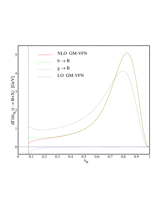
Figure 2: $d\Gamma(t\to B+X)/dx_{B}$ as a function of $x_{B}$ in the GM-VFN ($m_{b}\neq 0$) scheme including finite-$m_{B}$ corrections implemented with the energy scaling variable $z=E_{B}/E_{a}$ using Eq. (3). The NLO result (solid line) is compared to the LO one (dotted line) and broken up into the contributions due to $b\to B$ (dashed line) and $g\to B$ (dot-dashed line) fragmentation.

In Fig. 3, we study the improvement over previous calculations, at NLO in the ZM-VFN scheme neglecting $g\to B$ fragmentation and finite-$m_{B}$ corrections (dotted line), gained by switching to our preferred mode of evaluation, at NLO in the GM-VFN scheme including $g\to B$ fragmentation and finite-$m_{B}$ corrections (solid line). For comparison, we also show the full ZM-VFN prediction, including $g\to B$ fragmentation, for $m_{B}=0$ (dashed line). We observe from Fig. 3 that the improvement is threefold. First, the finite-$m_{B}$ corrections are responsible for the appearance of the threshold at $x_{B}=\rho_{B}=0.07783$. Second, $g\to B$ fragmentation leads to a significant reduction in size in the threshold region, as is familiar from Fig. 2. Third, the finite-$m_{b}$ corrections lead to a moderate reduction in size throughout the whole $x_{B}$ range allowed. A similar observation was made for the $x_{b}$ distribution in the perturbative-FF approach [9].

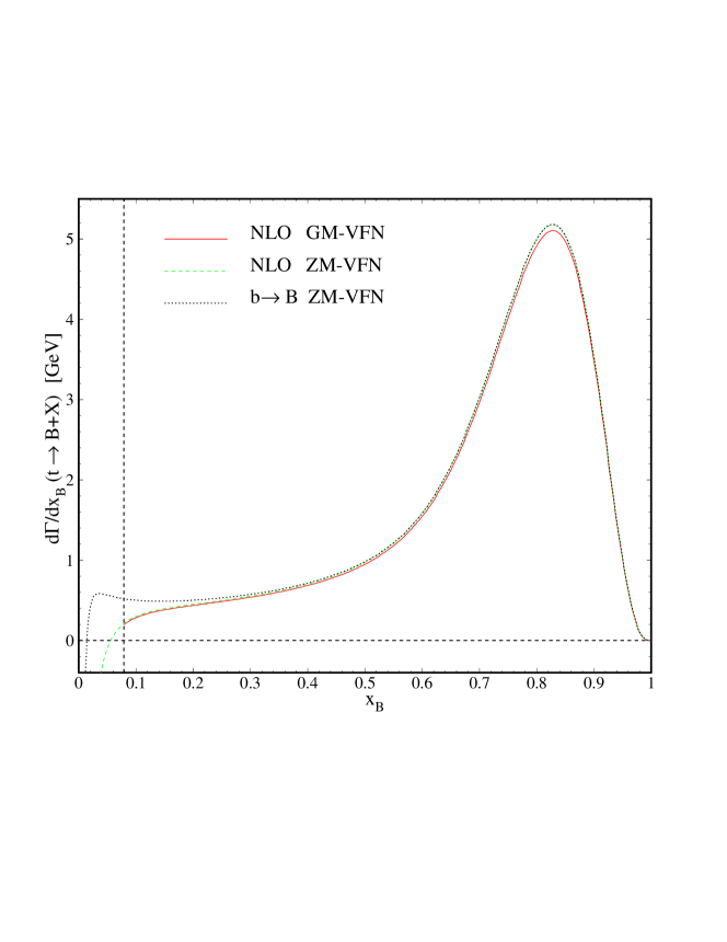
Figure 3: $d\Gamma(t\to B+X)/dx_{B}$ as a function of $x_{B}$ at NLO. The GM-VFN ($m_{b}\neq 0$) result including finite-$m_{B}$ corrections implemented with the energy scaling variable $z=E_{B}/E_{a}$ using Eq. (3) (solid line) is compared to the ZM-VFN ($m_{b}=0$) results for $m_{B}=0$ excluding (dotted line) and including (dashed line) $g\to B$ fragmentation.

For a more quantitative interpretation of Fig. 3, we consider in Fig. 4 the ZM-VFN result for $m_{B}=0$ without $g\to B$ fragmentation (dotted line) and the full GM-VFN result implemented with the energy scaling variable (solid line), both normalized to the full ZM-VFN result for $m_{B}=0$. We observe that the omission of $g\to B$ fragmentation entails an excess by a factor of up to 2 close to threshold, while the finite-$m_{b}$ corrections just amount to a few percent. This motivates us to adopt the ZM-VFN scheme including $g\to B$ fragmentation in the treatment of $d^{2}\Gamma(t\to B\ell^{+}\nu_{\ell}+X)/(dx_{B}\,d\cos\theta)$ below.

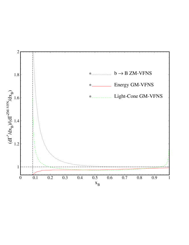
Figure 4: $d\Gamma(t\to B+X)/dx_{B}$ as a function of $x_{B}$ at NLO in the GM-VFN ($m_{b}\neq 0$) scheme including finite-$m_{B}$ corrections. The implementation with the energy scaling variable $z=E_{B}/E_{a}$ via Eq. (3) (solid line) is compared to the one with the light-cone-momentum scaling variable $z=p_{B}^{+}/p_{a}^{+}$ via Eq. (4) (dashed line). For comparison, also the ZM-VFN ($m_{b}=0$) result for $m_{B}=0$ excluding $g\to B$ fragmentation is shown (dotted line). All results are normalized to the ZM-VFN ($m_{b}=0$) one for $m_{B}=0$ including $g\to B$ fragmentation.

Figure 4 also includes the result obtained in the GM-VFN scheme implemented with the light-cone-momentum scaling variable $z=p_{B}^{+}/p_{a}^{+}$ via Eq. (4) (dashed line). Comparison with its counterpart for the energy scaling variable allows us to assess the theoretical uncertainty in the implementation of finite-$m_{B}$ corrections in the GM-VFN scheme. We observe from Fig. 4 that the two implementations of finite-$m_{B}$ corrections lead to very similar results over most of the $x_{B}$ range. Appreciable differences only appear close to the kinematical bounds. However, these should be taken with a grain of salt because the FFs used here [18] refer to the ZM-VFN scheme and do not carry any specific information on finite-$m_{B}$ effects and the scheme of their implementation.

In the remainder of this section, we consider the quantity $d^{2}\Gamma(t\to B\ell^{+}\nu_{\ell}+X)$ $/(dx_{B}\,d\cos\theta)$, which we study at NLO in the ZM-VFN scheme including $g\to B$ fragmentation and finite-$m_{B}$ corrections evaluated using the energy scaling variable. In Fig. 5, we present the $x_{B}$ distributions of $d\Gamma^{\lambda}/dx_{B}$ for $\lambda=0$ (solid line), $\lambda=-1$ (dashed line), and $\lambda=+1$ (dot-dashed line). For comparison, also the LO results for $\lambda=0,-1$ (dotted lines) are shown. As may be gleaned from Eq. (24), the latter amount to respectively $1/(1+2w)=69.59\%$ and $2w/(1+2w)=30.41\%$ of the LO result. In these two cases, the NLO corrections are similar in size and shape to the unpolarized case (see Fig. 2). As explained in Sec. 4, $\lambda=+1$ is prohibited at LO, which explains the smallness of the corresponding result.

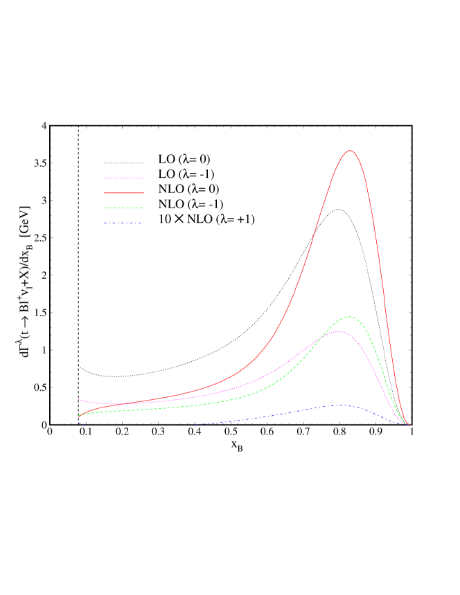
Figure 5: $d\Gamma^{\lambda}(t\to B\ell^{+}\nu_{\ell}+X)/dx_{B}$ as functions of $x_{B}$ in the ZM-VFN ($m_{b}=0$) scheme including finite-$m_{B}$ corrections implemented with the energy scaling variable $z=E_{B}/E_{a}$ using Eq. (3). The NLO results for $\lambda=0$ (solid line), $\lambda=-1$ (dashed line), and $\lambda=+1$ (dot-dashed line) and the LO results for $\lambda=0$ (upper dotted line) and $\lambda=-1$ (lower dotted line) are compared to each other.

6 Conclusions

Let alone its discovery potential with regard to the Higgs boson and new physics beyond the standard model, the LHC is a formidable top factory, which, among other things, will allow for the study of the dominant decay mode $t\to BW^{+}+X$ with unprecedented precision in the long run. In particular, this will enable us to deepen our understanding of the nonperturbative aspects of $B$-hadron formation by hadronization and to pin down the $b\to B$ and $g\to B$ FFs. The key observable for this purpose is the $x_{B}$ distribution $d\Gamma/dx_{B}$ of $t\to B+X$. By measuring the angular distribution of the $W$-boson decay products, also the three components $d\Gamma^{\lambda}/dx_{B}$ of $d\Gamma/dx_{B}$ corresponding to the polarization states $\lambda=0,\pm 1$ of the $W$ boson may be determined, which constrain these FFs even further.

We studied the quantity $d\Gamma/dx_{B}$ at NLO in the GM-VFN scheme [14, 15, 16, 17, 18] using nonperturbative $B$-hadron FFs determined by a global fit [18] of experimental data from the $Z$ factories [23, 24, 25], relying on their universality and scaling violations [19]. This allowed us to investigate for the first time finite-$m_{b}$ corrections and the contribution from gluon fragmentation to $d\Gamma/dx_{B}$. We also analyzed the size of finite-$m_{B}$ effects and their theoretical uncertainty due to the freedom in the choice of the scaling variable. Since the finite-$m_{b}$ effects turned out to so moderate, we neglected them, for simplicity, in our study of $d\Gamma^{\lambda}/dx_{B}$, which we treated at NLO in the ZM-VFN scheme taking into account finite-$m_{B}$ effects.

Comparing future measurements of $d\Gamma/dx_{B}$ and $d\Gamma^{\lambda}/dx_{B}$ at the LHC with our NLO predictions, we will be able to test the universality and scaling violations of the $B$-hadron FFs. These measurements will ultimately be the primary source of information on the $B$-hadron FFs. The formalism elaborated here is also applicable to the production of hadron species other than $B$ hadrons, e.g. pions, kaons, protons, $D$ mesons, etc., through top-quark decay.

Appendix

The coefficient functions $\hat{\Gamma}_{a}^{\lambda}$ in Eq. (19) exhibit the structure

$$\frac{1}{\Gamma_{0}}\,\frac{d\hat{\Gamma}_{a}^{0}}{dx_{a}} = \frac{1}{1+2w}\left[\delta_{ab}\delta(1-x_{a})+\frac{\alpha_{s}(\mu_{R})}{2\pi}\left(P_{ab}(x_{a})\ln\frac{m_{t}^{2}}{\mu_{F}^{2}}+C_{F}C_{a}^{0}(x_{a})\right)\right],$$

$$\frac{1}{\Gamma_{0}}\,\frac{d\hat{\Gamma}_{a}^{-}}{dx_{a}} = \frac{2w}{1+2w}\left[\delta_{ab}\delta(1-x_{a})+\frac{\alpha_{s}(\mu_{R})}{2\pi}\left(P_{ab}(x_{a})\ln\frac{m_{t}^{2}}{\mu_{F}^{2}}+C_{F}C_{a}^{-}(x_{a})\right)\right],$$

$$\frac{1}{\Gamma_{0}}\,\frac{d\hat{\Gamma}_{a}^{+}}{dx_{a}} = \frac{2w}{1+2w}\,\frac{\alpha_{s}(\mu_{R})}{2\pi}C_{F}C_{a}^{+}(x_{a}),$$ (24)

where

$$P_{qq}(x) = C_{F}\left(\frac{1+x^{2}}{1-x}\right)_{+},$$

$$P_{gq}(z) = C_{F}\frac{1+(1-x)^{2}}{x},$$ (25)

are the timelike $q\to q$ and $q\to g$ splitting functions at LO, respectively. Introducing the short-hand notation

$$w_{\pm}=1\pm\sqrt{w},$$ (26)

and defining

$$L_{1} = \ln(1-x)\theta\left(\frac{1}{w_{+}}-x\right)+\ln\left(\sqrt{w}x\right)\theta\left(x-\frac{1}{w_{+}}\right),$$

$$L_{2} = 2\ln\frac{1-x(1-w)}{\sqrt{w}}\theta\left(x-\frac{1}{w_{+}}\right),$$ (27)

where $\theta(x)=\int_{-\infty}^{x}dt\,\delta(t)$ is the Heaviside step function, we have

$$C_{b}^{0}(x) = -\delta(1-x)\left[4\mathop{\mathrm{Li}}\nolimits_{2}(w)+2\ln w\ln(1-w)+\frac{2w}{1-w}\ln w+3\frac{2+5w}{1+2w}\right]+\frac{1}{(1-x)_{+}}$$

$${}\times\left\{2(1+x^{2})\ln[x(1-w)]-2\frac{1+4w}{1+2w}\right\}+2(1+x^{2})\left[\frac{\ln(1-x)}{1-x}\right]_{+}-4wB_{1}$$

$${}-\frac{8w[4-x(3+w)]}{(1-w)(2-xw_{-})(2-xw_{+})}+\frac{1}{1+2w}\left(\frac{3+13w+8w^{2}}{1-w}-x\right),$$

$$C_{b}^{-}(x) = -\delta(1-x)\left[4\mathop{\mathrm{Li}}\nolimits_{2}(w)+2\ln w\ln(1-w)+\frac{2w}{1-w}\ln w+\frac{1-w}{w}\ln(1-w)\right.$$

$${}+\left.\frac{3(7+18w)}{4(1+2w)}\right]+\frac{1}{(1-x)_{+}}\left[2(1+x^{2})\ln[x(1-w)]-x^{3}\sqrt{\frac{1-w}{(2-xw_{-})(2-xw_{+})}}\right.$$

$${}-\left.\vphantom{\sqrt{\frac{1-w}{(2-xw_{-})(2-xw_{+})}}}\frac{4w}{1+2w}\right]+2(1+x^{2})\left[\frac{\ln(1-x)}{1-x}\right]_{+}-\left(\frac{1+w}{1-w}-x\right)\{L_{2}-\ln[1-x(1-w)]\}$$

$${}+B_{1}-\frac{1}{1-x}\left[B_{2}-\frac{x(2-7x+4x^{2})}{2(2-xw_{-})(2-xw_{+})}\right]+\frac{1-x}{1-x(1-w)}+\frac{3+x}{2}-\frac{1+x}{1+2w},$$

$$C_{b}^{+}(x) = \frac{3}{4}\delta(1-x)+\frac{x^{3}}{(1-x)_{+}}\sqrt{\frac{1-w}{(2-xw_{-})(2-xw_{+})}}+\left(\frac{1+w}{1-w}-x\right)$$ (28)

$${}\times\{L_{2}-\ln[1-x(1-w)]\}+B_{1}+\frac{1}{1-x}\left[B_{2}+\frac{x(6-9x+4x^{2})}{2(2-xw_{-})(2-xw_{+})}\right]$$

$${}+\frac{(1-x)[1+x(1-w)]}{2[1-x(1-w)]},$$

with

$$B_{1} = \frac{1}{2\sqrt{w}}\left[\frac{w_{+}(1-xw_{-})^{2}\left(2\sqrt{w}+xw_{-}^{2}\right)}{w_{-}(2-xw_{-})^{2}}\ln(1-xw_{-})+\frac{w_{-}(1-xw_{+})^{2}\left(2\sqrt{w}-xw_{+}^{2}\right)}{w_{+}(2-xw_{+})^{2}}\right.$$

$${}\times\left.\vphantom{\frac{w_{-}(1-xw_{+})^{2}\left(2\sqrt{w}-xw_{+}^{2}\right)}{w_{+}(2-xw_{+})^{2}}}\ln|1-xw_{+}|\right],$$

$$B_{2} = (1+x^{2})L_{1}+\sqrt{\frac{1-w}{(2-xw_{-})(2-xw_{+})}}$$ (29)

$${}\times\left\{\left[\frac{x^{2}(2-x)^{2}}{4(2-xw_{-})(2-xw_{+})}-\frac{x(1+x^{2})}{2}-\frac{x(12-11x)}{4(1-w)}+\frac{1-x}{(1-w)^{2}}\right]\right.$$

$$\times\left.\ln{\textstyle\frac{2-x\{1-3w+[2-x(1-w)]^{2}\}+(1-xw_{-})|1-xw_{+}|\sqrt{(1-w)(2-xw_{-})(2-xw_{+})}}{2-x(1+w)+\sqrt{(1-w)(2-xw_{-})(2-xw_{+})}}}-x^{3}\right\}$$

$$-\frac{(1-xw_{-})|1-xw_{+}|[2-x(1+w)]}{(1-w)(2-xw_{-})(2-xw_{+})}+\frac{1}{2(1-w)},$$

and

$$C_{g}^{0}(x) = \frac{1+(1-x)^{2}}{x}\left\{2\ln[(1-w)x(1-x)]+\frac{1}{1+2w}\right\}-4wG_{1}$$

$${}+\frac{1-x}{2x}\left\{\frac{1-x}{[1-x(1-w)]^{2}}-\frac{2(1+x)}{1-x(1-w)}+3(3+x)-\frac{16}{1-w}\right\}$$

$${}-\left[x-\frac{2(1+5w-2w^{2})}{1-w}+\frac{2(1+12w+3w^{2})}{x(1-w)^{2}}-\frac{16w(1+w)}{x^{2}(1-w)^{3}}\right]\ln[1-x(1-w)],$$

$$C_{g}^{-}(x) = 2\frac{1+(1-x)^{2}}{x}\left\{\ln[(1-w)x(1-x)]+\frac{1+w}{1+2w}\right\}+G_{1}-G_{2}$$

$${}-\frac{1}{1-w}\left[3-\frac{7+6w-2w^{2}}{x(1-w)}+\frac{4(1+2w)}{x^{2}(1-w)^{2}}\right]\ln[1-(1-w)x]$$

$${}-\frac{w[2-x(1-w)(2+w)]}{4(1-w)[1-x(1-w)]^{2}}-\frac{x}{4}+\frac{4-7w}{2(1-w)}-\frac{5-19w}{4x(1-w)},$$

$$C_{g}^{+}(x) = G_{1}+G_{2}-\left[x+\frac{1}{1-w}-\frac{5}{x(1-w)^{2}}+\frac{4}{x^{2}(1-w)^{3}}\right]\ln[1-(1-w)x]$$ (30)

$${}-\frac{w[2-x(1-w)(2+w)]}{4(1-w)[1-x(1-w)]^{2}}+\frac{3}{4}x-\frac{4-w}{2(1-w)}+\frac{5-3w}{4x(1-w)},$$

with

$$G_{1} = \frac{1}{2x^{2}\sqrt{w}}\left[\frac{w_{+}(1-xw_{-})^{2}(2-xw_{-}^{2})}{w_{-}^{3}}\ln(1-xw_{-})-\frac{w_{-}(1-xw_{+})^{2}(2-xw_{+}^{2})}{w_{+}^{3}}\right.$$

$${}\times\left.\vphantom{\frac{w_{+}(1-xw_{-})^{2}(2-xw_{-}^{2})}{w_{-}^{3}}}\ln|1-xw_{+}|\right],$$

$$G_{2} = \frac{1+(1-x)^{2}}{x}L_{1}+\left[\frac{x}{2}-\frac{1}{1-w}+\frac{1+3w-w^{2}}{x(1-w)^{2}}-\frac{4w}{x^{2}(1-w)^{3}}\right]L_{2}$$ (31)

$${}+\frac{(1-xw_{-})|1-xw_{+}|}{4[1-x(1-w)]^{2}}\left[x(1-w)-2(2+w)+\frac{7(1+w)}{x(1-w)}-\frac{4(1+w)}{x^{2}(1-w)^{2}}\right]$$

$${}+\frac{1+w}{x^{2}(1-w)^{2}}.$$

References

-
[1]
S. Moch, P. Uwer,
Phys. Rev. D 78 (2008) 034003,
arXiv:0804.1476 [hep-ph];
M. Cacciari, S. Frixione, M.L. Mangano, P. Nason, G. Ridolfi, JHEP 0809 (2008) 127, arXiv:0804.2800 [hep-ph];
N. Kidonakis, R. Vogt, Phys. Rev. D 78 (2008) 074005, arXiv:0805.3844 [hep-ph]. -
[2]
N. Cabibbo,
Phys. Rev. Lett. 10 (1963) 531;
M. Kobayashi, T. Maskawa, Prog. Theor. Phys. 49 (1973) 652. - [3] W. Bernreuther, J. Phys. G 35 (2008) 083001, arXiv:0805.1333 [hep-ph].
- [4] M. Jeżabek, J.H. Kühn, Nucl. Phys. B 314 (1989) 1.
-
[5]
M. Jeżabek, J.H. Kühn,
Nucl. Phys. B 320 (1989) 20;
M. Jeżabek, J.H. Kühn, Phys. Rev. D 48 (1993) 1910, arXiv:hep-ph/9302295;
M. Jeżabek, J.H. Kühn, Phys. Rev. D 49 (1994) 4970 (Erratum);
A. Czarnecki, Phys. Lett. B 252 (1990) 467;
C.S. Li, R.J. Oakes, T.C. Yuan, Phys. Rev. D 43 (1991) 3759. -
[6]
A. Czarnecki, K. Melnikov,
Nucl. Phys. B 544 (1999) 520,
arXiv:hep-ph/9806244;
K.G. Chetyrkin, R. Harlander, T. Seidensticker, M. Steinhauser, Phys. Rev. D 60 (1999) 114015, arXiv:hep-ph/9906273;
I.R. Blokland, A. Czarnecki, M. Ślusarczyk, F. Tkachov, Phys. Rev. Lett. 93 (2004) 062001, arXiv:hep-ph/0403221;
I.R. Blokland, A. Czarnecki, M. Ślusarczyk, F. Tkachov, Phys. Rev. D 71 (2005) 054004, arXiv:hep-ph/0503039;
I.R. Blokland, A. Czarnecki, M. Ślusarczyk, F. Tkachov, Phys. Rev. D 79 (2009) 019901 (Erratum);
R. Bonciani, A. Ferroglia, JHEP 0811 (2008) 065, arXiv:0809.4687 [hep-ph]. - [7] T. Mehen, Phys. Lett. B 417 (1998) 353, arXiv:hep-ph/9707403.
-
[8]
A. Denner, T. Sack,
Nucl. Phys. B 358 (1991) 46;
G. Eilam, R.R. Mendel, R. Migneron, A. Soni, Phys. Rev. Lett. 66 (1991) 3105;
C.-P. Yuan, T.C. Yuan, Phys. Rev. D 44 (1991) 3603;
T. Kuruma, Z. Phys. C 57 (1993) 551;
S.M. Oliveira, L. Brücher, R. Santos, A. Barroso, Phys. Rev. D 64 (2001) 017301, arXiv:hep-ph/0011324. - [9] G. Corcella, A.D. Mitov, Nucl. Phys. B 623 (2002) 247, arXiv:hep-ph/0110319.
- [10] M. Cacciari, G. Corcella, A.D. Mitov, JHEP 0212 (2002) 015, arXiv:hep-ph/0209204.
-
[11]
G. Corcella, F. Mescia,
Eur. Phys. J. C 65 (2010) 171,
arXiv:0907.5158 [hep-ph];
G. Corcella, F. Mescia, Eur. Phys. J. C 68 (2010) 687 (Erratum);
S. Biswas, K. Melnikov, M. Schulze, JHEP 1008 (2010) 048, arXiv:1006.0910 [hep-ph]. -
[12]
B. Mele, P. Nason,
Nucl. Phys. B 361 (1991) 626;
J.P. Ma, Nucl. Phys. B 506 (1997) 329, arXiv:hep-ph/9705446;
S. Keller, E. Laenen, Phys. Rev. D 59 (1999) 114004, arXiv:hep-ph/9812415;
M. Cacciari, S. Catani, Nucl. Phys. B 617 (2001) 253, arXiv:hep-ph/0107138;
K. Melnikov, A. Mitov, Phys. Rev. D 70 (2004) 034027, arXiv:hep-ph/0404143;
A. Mitov, Phys. Rev. D 71 (2005) 054021, arXiv:hep-ph/0410205. -
[13]
V.N. Gribov, L.N. Lipatov,
Sov. J. Nucl. Phys. 15 (1972) 438
[Yad. Fiz. 15 (1972) 781];
G. Altarelli, G. Parisi, Nucl. Phys. B 126 (1977) 298;
Yu.L. Dokshitzer, Sov. Phys. JETP 46 (1977) 641 [Zh. Eksp. Teor. Fiz. 73 (1977) 1216]. - [14] T. Kneesch, B.A. Kniehl, G. Kramer, I. Schienbein, Nucl. Phys. B 799 (2008) 34, arXiv:0712.0481 [hep-ph].
-
[15]
G. Kramer, H. Spiesberger,
Eur. Phys. J. C 22 (2001) 289,
arXiv:hep-ph/0109167;
G. Kramer, H. Spiesberger, Eur. Phys. J. C 28 (2003) 495, arXiv:hep-ph/0302081. -
[16]
G. Kramer, H. Spiesberger,
Eur. Phys. J. C 38 (2004) 309,
arXiv:hep-ph/0311062;
B.A. Kniehl, G. Kramer, I. Schienbein, H. Spiesberger, Eur. Phys. J. C 62 (2009) 365, arXiv:0902.3166 [hep-ph];
G. Kramer, H. Spiesberger, Phys. Lett. B 679 (2009) 223, arXiv:0906.2533 [hep-ph]. -
[17]
B.A. Kniehl, G. Kramer, I. Schienbein, H. Spiesberger,
Phys. Rev. D 71 (2005) 014018,
arXiv:hep-ph/0410289;
B.A. Kniehl, G. Kramer, I. Schienbein, H. Spiesberger, Eur. Phys. J. C 41 (2005) 199, arXiv:hep-ph/0502194;
B.A. Kniehl, G. Kramer, I. Schienbein, H. Spiesberger, Phys. Rev. Lett. 96 (2006) 012001, arXiv:hep-ph/0508129;
B.A. Kniehl, G. Kramer, I. Schienbein, H. Spiesberger, Phys. Rev. D 79 (2009) 094009, arXiv:0901.4130 [hep-ph];
B.A. Kniehl, G. Kramer, I. Schienbein, H. Spiesberger, Phys. Rev. D 84 (2011) 094026, arXiv:1109.2472 [hep-ph];
B.A. Kniehl, G. Kramer, I. Schienbein, H. Spiesberger, Report Nos. DESY 12–013, MZ–TH/12–07, LPSC 12019, arXiv:1202.0439 [hep-ph]. - [18] B.A. Kniehl, G. Kramer, I. Schienbein, H. Spiesberger, Phys. Rev. D 77 (2008) 014011, arXiv:0705.4392 [hep-ph].
- [19] J.C. Collins, Phys. Rev. D 58 (1998) 094002, arXiv:hep-ph/9806259.
-
[20]
S. Albino, B.A. Kniehl, G. Kramer, W. Ochs,
Phys. Rev. D 73 (2006) 054020,
arXiv:hep-ph/0510319;
S. Albino, B.A. Kniehl, G. Kramer, C. Sandoval, Phys. Rev. D 75 (2007) 034018, arXiv:hep-ph/0611029;
S. Albino, B.A. Kniehl, G. Kramer, Nucl. Phys. B 803 (2008) 42, arXiv:0803.2768 [hep-ph]. - [21] M. Fischer, S. Groote, J.G. Körner, M.C. Mauser, Phys. Rev. D 63 (2001) 031501(R), arXiv:hep-ph/0011075.
- [22] K. Nakamura, et al., Particle Data Group, J. Phys. G 37 (2010) 075021.
- [23] A. Heister, et al., ALEPH Collaboration, Phys. Lett. B 512 (2001) 30, arXiv:hep-ex/0106051.
- [24] G. Abbiendi, et al., OPAL Collaboration, Eur. Phys. J. C 29 (2003) 463, arXiv:hep-ex/0210031.
-
[25]
K. Abe, et al., SLD Collaboration,
Phys. Rev. Lett. 84 (2000) 4300,
arXiv:hep-ex/9912058;
K. Abe, et al., SLD Collaboration, Phys. Rev. D 65 (2002) 092006, arXiv:hep-ex/0202031;
K. Abe, et al., SLD Collaboration, Phys. Rev. D 66 (2002) 079905 (Erratum).