Multiwavelength Campaign on Mrk 509

Abstract

Aims. Active Galactic Nuclei often show evidence of photoionized outflows. A major uncertainty in models for these outflows is the distance ($R$) to the gas from the central black hole. In this paper we use the HST/COS data from a massive multi-wavelength monitoring campaign on the bright Seyfert I galaxy Mrk 509, in combination with archival HST/STIS data, to constrain the location of the various kinematic components of the outflow.

Methods. We compare the expected response of the photoionized gas to changes in ionizing flux with the changes measured in the data using the following steps: 1) We compare the column densities of each kinematic component measured in the 2001 STIS data with those measured in the 2009 COS data; 2) We use time-dependent photionization calculations with a set of simulated lightcurves to put statistical upper limits on the hydrogen number density ($n_{\scriptscriptstyle H}$) that are consistent with the observed small changes in the ionic column densities; 3) From the upper limit on $n_{\scriptscriptstyle H}$, we calculate a lower limit on the distance to the absorber from the central source via the prior determination of the ionization parameter. Our method offers two improvements on traditional timescale analysis. First, we account for the physical behavior of AGN lightcurves. Second, our analysis accounts for the quality of measurement in cases where no changes are observed in the absorption troughs.

Results. The very small variations in trough ionic column densities (mostly consistent with no change) between the 2001 and 2009 epochs allow us to put statistical lower limits on $R$ between 100–200 pc for all the major UV absorption components at a confidence level of 99%. These results are mainly consistent with the independent distance estimates derived for the warm absorbers from the simultaneous X-ray spectra. Based on the 100–200 pc lower limit for all the UV components, this absorber cannot be connected with an accretion disc wind. The outflow might have originated from the disc, but based on simple ballistic kinematics, such an event had to occur at least 300,000 years ago in the rest frame of the source.

1 Introduction

Outflows from active galactic nuclei (AGN) are detected as blue-shifted spectral absorption features with respect to the rest frame of the AGN (e.g., Crenshaw et al. 2000, 2003; Kriss et al. 2000; Arav et al. 2002). Measurements of the absorption troughs, combined with photoionization modeling, yield the ionization parameter ($U_{H}$) and total column density of the gas ($N_{H}$). However spectral data do not provide a direct measurement for the distance ($R$) to the outflow from the central source, and most outflows are unresolved point sources on images. Therefore, we use indirect methods to obtain $R$, where the most common ones use the relationship $U_{H}\propto(n_{\scriptscriptstyle H}R^{2})^{-1}$. Since $U_{H}$ can be determined from photoionization modeling, knowledge of the hydrogen number density ($n_{\scriptscriptstyle H}$) yields $R$.

In spectra where absorption features due to excited states of a given ion are detected, the ratio of column densities from excited and ground levels can yield $n_{\scriptscriptstyle H}$ (e.g., de Kool et al. 2001; Hamann et al. 2001; Korista et al. 2008; Moe et al. 2009; Dunn et al. 2010a; Edmonds et al. 2011). Alternatively, determining how the absorber responds to changes in the ionizing flux can provide reliable estimates of $n_{\scriptscriptstyle H}$. Time-variability of the continuum is a known feature of AGN (e.g., Uttley et al. 2003; McHardy et al. 2006; Ishibashi & Courvoisier 2009). How the fractional population of each ion in the outflowing gas changes in response to variation in the ionizing continuum depends on the electron number density $n_{e}$, which is $\simeq 1.2n_{\scriptscriptstyle H}$ in highly ionized gas. The time in which the absorber adjusts to the new flux level is inversely proportional to $n_{e}$. Therefore, by tracking changes in ionic column densities and ionizing flux over time we can estimate $n_{\scriptscriptstyle H}$ and thus, the distance (e.g. Nicastro et al. 1999; Gabel et al. 2005).

As part of a large multiwavelength campaign (Kaastra et al. 2011, hereafter Paper I), the bright Seyfert I galaxy Mrk 509 was observed with the Cosmic Origins Spectrograph (COS) onboard the Hubble Space Telescope (for details, see Kriss et al. 2011, hereafter Paper VI). Since the Mrk 509 UV spectra do not contain troughs from excited states, we use time-variability to constrain the distance to the absorber. This is done by: 1) comparing the column densities of each kinematic component measured in the 2001 STIS data (Kraemer et al. 2003) to those measured in the 2009 COS data (Paper VI); 2) determining the upper limit on $n_{\scriptscriptstyle H}$ that is consistent with the small observed changes in the ionic column densities. From the upper limit on $n_{\scriptscriptstyle H}$, we then calculate the lower limit on $R$ via the determined $U_{H}$. This method has been applied to the Mrk 509 X-ray data by Kaastra et al. (2012, hereafter Paper VIII) using the observed lightcurve over a 100 day monitoring campaign. Since the lightcurve for Mrk 509 was was not monitored between the the 2001 STIS epoch and the start of our campaign, we use Monte Carlo simulations to develop a sample of lightcurves to put statistical limits on $n_{\scriptscriptstyle H}$. In section 6, we will show the limits derived from timescale arguments are similar to and bracket our statistical limits.

The paper is structured as follows. In section 2, we discuss the measurements of and changes in absorption troughs between the 2001 and 2009 epochs. Photoionization solutions are given in section 3, and time-dependent ionization is discussed in section 4. The simulations used to determine $n_{\scriptscriptstyle H}$ are discussed in section 5 along with distance determinations. We discuss our results in section 6. In the appendix, we provide an illustrative example of the time-dependent photoionization equations for the case of hydrogen, which can be solved analytically.

2 Comparison of UV Spectra from the 2001 and 2009 Epochs

To quantitatively establish differences in UV absorption between the epochs of the STIS observation (2001 April 13) and the COS observations (2009 December 10 and 11), we use the calibrated COS and STIS spectra presented in Paper VI. For STIS, the spectrum is the one-dimensional archival echelle spectrum originally obtained by Kraemer et al. (2003), re-reduced with up-to-date pipeline processing that includes corrections for scattered light and echelle blaze evolution. In Paper VI, we discuss custom calibrations for the COS spectrum that include improved wavelength calibrations (accurate to 5 $\rm km\leavevmode\nobreak\ s^{-1}$), flat field, and flux calibrations. In addition, the COS spectrum was deconvolved (see Paper VI) to correct for the broad wings of the line-spread function in COS (Ghavamian et al. 2009; Kriss 2011). As we showed in Paper VI, this deconvolution is important for an accurate comparison between the COS and STIS spectra. Comparison of the depths and widths of interstellar lines that are common to the COS and STIS spectra (e.g., Figure 3 in Paper VI) give us confidence that the deconvolved COS spectrum is an accurate measure of the spectral properties of Mrk 509—saturated ISM lines in the COS spectrum are black and have the same width as in the STIS spectrum, and unsaturated lines have the same depth and width.

The calibrated spectra were divided by the best fitting emission model, which includes continuum and emission lines (presented in Paper VI). The same emission model was used for both STIS and COS spectra, but with appropriately fitted adjustments to the intensities of the emission lines and the continuum. We then rebinned these spectra onto the identical velocity scale using velocity bins of 5 $\rm km\leavevmode\nobreak\ s^{-1}$. This scale combines multiple pixels in each bin for both STIS and COS spectra, reducing the correlated errors introduced when dividing original pixels between adjacent velocity bins. This scale also gives about 3 bins per COS resolution element, so we preserve the full resolution of the COS spectrum. The Ly$\alpha$ absorption trough in Mrk 509 is heavily saturated, with differences in absorption dominated by differences in covering fraction rather than optical depth. We therefore confine our analysis to the unsaturated N v, Si iv, and C iv absorption lines. Fig. 1 compares the STIS and COS absorption troughs for each transition of N v, Si iv, and C iv. We note that due to the close spacing of the C iv $\lambda\lambda 1548,1550$ doublet, the troughs of these transitions overlap in velocity in the ranges $-498$ to $-375\leavevmode\nobreak\ \rm km\leavevmode\nobreak\ s^{-1}$ and $+75$ to $+260\leavevmode\nobreak\ \rm km\leavevmode\nobreak\ s^{-1}$. In Paper VI, the absorption in the COS spectrum was fit using 14 Gaussian components. For comparing column densities, we use the N v profiles to define 9 independent troughs with velocity boundaries as given in Table LABEL:coldensi.

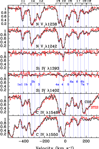
Figure 1: Comparison of spectral features in the COS (black) and STIS (red) spectra of Mrk 509. Normalized relative fluxes are plotted as a function of velocity relative to the systemic redshift of $z=0.034397$. The boundaries of the 9 absorption troughs used in our analysis are shown along the top (see Table LABEL:coldensi). The centroids of the individual Gaussian components identified in Paper VI are shown by the vertical dotted blue lines.

There was an overall increase in flux for the COS spectrum compared to the STIS spectrum, with an average increase of 72% (see Paper VI for details). For comparison to the historical lightcurve for Mrk 509, at rest wavelength 1354 $\AA$, $F_{\lambda}$(STIS)$=0.849\times 10^{-13}$ erg cm^-2 s^-1 $\AA^{-1}$, $F_{\lambda}$(COS)$=1.46\times 10^{-13}$ erg cm^-2 s^-1 $\AA^{-1}$, and the mean flux of the lightcurve given in Section 5, Figure 3 is $F_{\lambda}$(mean)$=0.704\times 10^{-13}$ erg cm^-2 s^-1 $\AA^{-1}$.

2.1 absorption trough variability

To make a quantitative comparison between the COS and STIS spectra, for each trough in each spectrum we calculate the mean transmission

$$\left<T\right>={{\sum T_{i}}\over{N}},$$ (1)

where $T_{i}$ is the transmission in velocity bin $i$, and $N$ is the total number of bins in a trough. We also calculate the mean observed difference in transmission between the COS and STIS spectra, $\left<T_{C}-T_{S}\right>$, and the mean error in this difference,

$$\left<\sigma\right>={{\sqrt{\sum(\sigma_{i,COS}^{2}+\sigma_{i,STIS}^{2})}}\over{N}}.$$ (2)

Due to the high S/N of the COS data, the error in the difference is dominated by the statistical errors in the STIS spectrum. Table LABEL:coldensi gives the mean transmissions of each trough as observed in the COS spectrum, the mean fractional difference between the COS and STIS troughs normalized by the mean COS transmission, and the mean fractional error in this difference, again normalized by the mean COS transmission.

As one can see in Figure 1 and Table LABEL:coldensi, the absorption in Mrk 509 showed little variation between the 2001 STIS spectrum and the 2009 COS spectrum. Our criterion for a significant variation requires that both the red and the blue components of a trough show a difference of $>2\sigma$. In Table LABEL:coldensi, this means that the absolute value in the last column is greater than 2. In Paper VI, we noted a significant difference in the N v absorption in trough T1, and that is apparent in the comparison shown in Table LABEL:coldensi. Both the red and blue doublets of N v show more than a $2\sigma$ difference in transmission between the COS and STIS spectra. However, no other trough in N v or Si iv meets this criterion, and only trough T2 in C iv shows such a significant difference.

Table 1: variability in mrk 509 absorption troughs

Feature	Trough	$v_{1}$	$v_{2}$	$\left<T_{C}\right>$	$\left<T_{C}-T_{S}\right>/\left<T_{C}\right>$	$\left<\sigma\right>/\left<T_{C}\right>$	$\left<T_{C}-T_{S}\right>/\left<\sigma\right>$
N v $\lambda$ 1238	T1	-425	-385	0.605	-0.182	0.039	-4.7
N v $\lambda$ 1238	T2	-350	-270	0.425	0.004	0.035	0.1
N v $\lambda$ 1238	T3	-265	-210	0.669	0.030	0.031	1.0
N v $\lambda$ 1238	T4	-90.0	-45.0	0.530	-0.044	0.042	-1.1
N v $\lambda$ 1238	T5	-40.0	15.0	0.249	-0.092	0.065	-1.4
N v $\lambda$ 1238	T6	20.0	70.0	0.664	-0.023	0.030	-0.8
N v $\lambda$ 1238	T7	95.0	155	0.647	-0.005	0.028	-0.2
N v $\lambda$ 1238	T8	165	200	0.825	0.020	0.030	0.6
N v $\lambda$ 1238	T9	205	250	0.831	-0.079	0.027	-3.0
N v $\lambda$ 1242	T1	-425	-385	0.715	-0.092	0.030	-3.0
N v $\lambda$ 1242	T2	-350	-270	0.590	0.013	0.023	0.5
N v $\lambda$ 1242	T3	-265	-210	0.774	0.008	0.024	0.3
N v $\lambda$ 1242	T4	-90.0	-45.0	0.688	-0.052	0.027	-1.9
N v $\lambda$ 1242	T5	-40.0	15.0	0.376	-0.096	0.039	-2.4
N v $\lambda$ 1242	T6	20.0	70.0	0.798	-0.034	0.024	-1.4
N v $\lambda$ 1242	T7	95.0	155	0.774	-0.049	0.023	-2.2
N v $\lambda$ 1242	T8	165	200	0.901	-0.027	0.026	-1.0
N v $\lambda$ 1242	T9	205	250	0.916	0.003	0.022	0.1
Si iv $\lambda$ 1393	T5	-45.0	15.0	0.937	0.006	0.023	0.3
Si iv $\lambda$ 1402	T5	-45.0	15.0	0.987	0.060	0.021	2.9
C iv $\lambda$ 1548	T1	-425	-395	0.643	0.060	0.034	1.8
C iv $\lambda$ 1548	T2	-350	-270	0.294	0.190	0.035	5.5
C iv $\lambda$ 1548	T3	-265	-200	0.613	0.010	0.023	4.3
C iv $\lambda$ 1548	T4	-90.0	-45.0	0.475	0.101	0.030	3.4
C iv $\lambda$ 1548	T5	-40.0	15.0	0.261	0.120	0.041	2.9
C iv $\lambda$ 1548	T6	20.0	70.0	0.694	-0.007	0.024	-0.3
C iv $\lambda$ 1548	T7	95.0	155	0.601	0.017	0.023	0.8
C iv $\lambda$ 1548	T8	165	200	0.246	0.118	0.047	2.5
C iv $\lambda$ 1548	T9	205	250	0.486	0.009	0.029	0.3
C iv $\lambda$ 1550	T1	-425	-395	0.562	-0.010	0.033	-0.3
C iv $\lambda$ 1550	T2	-350	-270	0.404	0.070	0.024	2.9
C iv $\lambda$ 1550	T3	-265	-200	0.749	0.026	0.019	1.4
C iv $\lambda$ 1550	T4	-90.0	-45.0	0.663	0.024	0.023	1.1
C iv $\lambda$ 1550	T5	-40.0	15.0	0.368	0.036	0.031	1.2
C iv $\lambda$ 1550	T6	20.0	70.0	0.829	-0.021	0.020	-1.1
C iv $\lambda$ 1550	T7	95.0	155	0.881	0.004	0.018	0.2
C iv $\lambda$ 1550	T8	165	200	0.971	-0.090	0.023	-3.9
C iv $\lambda$ 1550	T9	205	250	0.978	-0.029	0.020	-1.4

2.2 column density determination

For each epoch, we determine the ionic column densities associated with the nine components (T1–T9) shown in Figure 1 by modeling the residual intensity observed accross the absorption troughs. Assuming a single homogeneous emission source $F_{0}$ whose spatial extension is normalized to 1, the transmitted flux $F_{i}(v)$ for a line $i$ can be written as

$$F_{i}(v)=F_{0}(\lambda(v))\int_{0}^{1}e^{-\tau_{i}(x,v)}dx$$ (3)

where $v$ is the radial velocity of the outflow and $\tau_{i}(x,v)$ is the optical depth of the absorber accross the emission source. In this relation, we implicitly reduced the number of spatial dimensions from two to one. This assumption, whose validity is discussed in Arav et al. (2005), allows us to derive meaningful quantities from the fitting of residual intensity profiles. We consider two common models for the absorber: the apparent optical depth (AOD) model where the absorbing material is simply characterized by $\tau_{i}(x,v)=\tau_{i}(v)$ and fully covers the emission source, and the partial-covering (PC) model in which the material with $\tau_{i}(v)$ only covers a fraction $C(v)$ of the emission source at a given velocity. Once computed over the width of the trough, the optical depth solution $\tau_{i}(x,v)$ is transformed into column density using the relation

$$N_{ion}(v)=\frac{3.8\times 10^{14}}{f_{i}\lambda_{i}}<\tau_{i}(v)>\leavevmode\nobreak\ (\mathrm{cm}^{-2}\>\mathrm{km}^{-1}\>\mathrm{s})$$ (4)

where $f_{i}$, $\lambda_{i}$ and $<\tau_{i}(v)>$ are respectively the oscillator strength, the rest wavelength and the average optical depth accross the emission source of line $i$ (see Edmonds et al. 2011 for details). The main uncertainty in the fitting procedure, and thus in the derived column density, comes from the assumption about the spatial distribution of the absorbing material.

The PC model is considered in order to account for the fact that in AGN, when one observes at least two lines from the same ion, the apparent optical depth ratio $R_{ij}^{app}$ between the lines $i$ and $j$ does not always follow the expected laboratory value $R_{ij}^{lab}=\lambda_{i}f_{i}/\lambda_{j}f_{j}$. This observation can be explained if the absorber only partially covers the emission source (e.g. Hamann et al. 1997; Arav et al. 1999). In the case of doublet lines like C iv, N v, and Si iv, $R_{br}^{lab}\simeq 2$; i.e., the blue transition of the doublet is twice as strong as the red one. Therefore, the residual intensity in the blue line should lie between $I_{b}=I_{r}^{2}$ (AOD model) and $I_{b}=I_{r}$ (fully saturated trough in the PC model). In the upper panels of Fig. 2 we plot the COS C iv and N v line profiles as well as the expected residual intensity for the strongest transition assuming the AOD scenario, highlighting the allowed physical range of values for $I_{b}$ based on the observation of $I_{r}$. While several kinematic components show a significant departure from the AOD prediction, suggesting a partial covering of the emission source, none of the unblended components exhibits a strong saturation effect (i.e. $I_{b}\simeq I_{r}$) with the exception of C iv in component T1. This allows us to determine accurate ionic column densities as well as quantitatively examine the variations in the absorber between the STIS and the COS epochs.

In the lower panels of Fig. 2 we display the $N_{ion}(v)$ solution derived for C iv and N v for the COS epoch for both the AOD (computed on the weakest line of the doublet) and PC absorber models. The PC solution can only be computed if one observes at least two unblended lines from the same ion. Given the blending of the blue C iv line in trough T7 and the non-detection of C iv in troughs T8 and T9 we do not report column for these troughs using the PC model, but only provide a lower limit based on the AOD model. Trough T1 is strongly saturated in C iv as revealed by the perfect match of the shape of the blue and red component line profiles. This only allows us to place a conservative lower limit on the column density by assuming an optical depth of at least $\tau=4$ across the line profile of the red component. Looking at the Si iv line profile, only detected in trough T5, reveals an optically thin absorption line with a covering of unity accross the trough. We corrected the PC solution in several velocity bins by using the mean PC solution derived in the adjacent pixels in order to account for the increased sensitivity of the PC solution to the noise when modeling the shallower parts of the troughs. These points are marked with crosses in Fig. 2.

We list the integrated values of the computed column densities across the nine independent components using both absorber models in Table LABEL:line_data. Except for C iv in component T1, the integrated column densities obtained using the two absorber models are generally in agreement (with differences $\raisebox{-2.15277pt}{$\;\stackrel{{\scriptstyle<}}{{\sim}}\;$}30\%$) for both STIS and COS data lending further support to the non-saturation of the components. A higher discrepancy is generally observed for shallow troughs in the STIS spectrum and is explained by the lower S/N in that dataset (cf. the Si iv measurement). In Table LABEL:line_data, we also provide the differences in column densities determined between the COS and STIS epochs as well as the fractional differences in column densities normalized to the COS measurement for both absorber models. One can see that the fractional differences observed are in general agreement between both absorber models, as already suggested by the small difference in computed column density typical of non-saturated troughs.

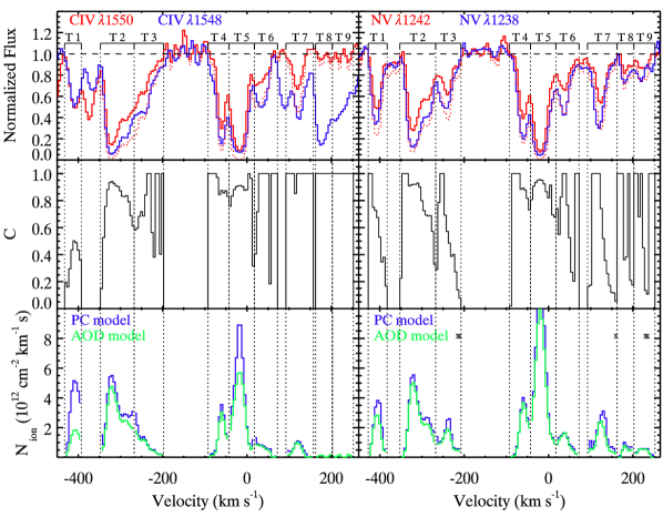
Figure 2: The upper panel presents the line profiles associated to C iv and N v in the COS spectrum. The dotted red line, only plotted in regions free of known blending in the weakest transition (red line), represents the expected residual intensity in the stronger transition (blue line) assuming an absorber totally covering the emission source (AOD model, $I_{b}=I_{r}^{2}$). The central panel shows the derived covering solution obtained for C iv and N v as a function of the radial velocity. A high covering is observed in most components of the outflow, while trough T1 presents a lower covering in both C iv and N v. The low covering derived in troughs T6 and T7 of N v is most likely due to a shift in the wavelength solution. In the lower panel we plot the ionic column density solution derived for both ions. The AOD model solution is computed on the red component of the doublet. Velocity bins in which the PC solution has been corrected to account for the shallowness of the trough are denoted with crosses (see text).

Table 2: computed column densities

		AOD				PC
Trough	Ion	C	S	C-S	(C-S)/C	C	S	C-S	(C-S)/C
T1	N(C iv)	$>$ 47.1	$>$ 39.0	$\cdots$	$\cdots$	$>$ 135	$>$ 101	$\cdots$	$\cdots$
T1	N(N v)	64.8$\pm 0.8$	48.6$\pm 5.0$	16.2	0.25$\pm 0.08$	86.4$\pm 1.5$	70.7${}^{+18}_{-8.7}$	15.8	0.18${}^{+0.21}_{-0.10}$
T2	N(C iv)	227$\pm 1$	252$\pm 8$	-25	-0.11$\pm 0.03$	264$\pm 1$	288${}^{+54}_{-13}$	-24.0	-0.09${}^{+0.20}_{-0.05}$
T2	N(N v)	201$\pm 1$	215$\pm 10$	-14	-0.07$\pm 0.05$	225$\pm 1$	254${}^{+480}_{-13}$	-28.4	-0.13${}^{+2.1}_{-0.06}$
T3	N(C iv)	56.0$\pm 0.4$	61.4$\pm 3.4$	-5.4	-0.10$\pm 0.06$	68.9$\pm 0.7$	67.9$\pm 3.9$	1.0	0.01$\pm 0.06$
T3	N(N v)	62.2$\pm 0.8$	64.6$\pm 5.6$	-2.5	-0.04$\pm 0.09$	78.0$\pm 1.2$	84.5${}^{+670}_{-8.9}$	-6.5	-0.08${}^{+8.6}_{-0.16}$
T4	N(C iv)	64.1$\pm 0.5$	71.4$\pm 3.4$	-7.3	-0.11$\pm 0.05$	72.7$\pm 0.5$	76.5$\pm 3.1$	-3.8	-0.05$\pm 0.04$
T4	N(N v)	84.7$\pm 0.9$	78.5$\pm 5.4$	6.1	0.07$\pm 0.06$	92.7${}^{+38}_{-0.8}$	91.2${}^{+8.4}_{-6.4}$	1.5	0.02${}^{+0.42}_{-0.07}$
T5	N(C iv)	197$\pm 1$	211$\pm 10$	-13	-0.07$\pm 0.05$	264$\pm 4$	266${}^{+69}_{-13}$	-2.0	-0.01${}^{+0.26}_{-0.05}$
T5	N(N v)	299$\pm 2$	272${}^{+22}_{-14}$	28	0.09${}^{+0.08}_{-0.05}$	356$\pm 5$	346${}^{+2500}_{-34}$	10.2	0.03${}^{+6.9}_{-0.10}$
T5	N(Si iv)	2.7$\pm 0.2$	4.6${}^{+1.4}_{-1.0}$	-2.0	-0.74${}^{+0.54}_{-0.38}$	2.8${}^{+21}_{-0.1}$	9.5${}^{+43}_{-1.9}$	-6.7	-2.5${}^{+31}_{-0.7}$
T6	N(C iv)	28.2$\pm 0.4$	28.9$\pm 2.7$	-0.7	-0.03$\pm 0.10$	33.7$\pm 0.5$	35.3${}^{+5.6}_{-3.4}$	-1.6	-0.05${}^{+0.17}_{-0.10}$
T6	N(N v)	50.6$\pm 0.8$	48.4$\pm 4.9$	2.3	0.04$\pm 0.10$	54.8$\pm 0.7$	53.6$\pm 3.8$	1.2	0.02$\pm 0.07$
T7	N(C iv)	24.9$\pm 0.4$	27.7$\pm 2.8$	-2.8	-0.11$\pm 0.12$	$\cdots$	$\cdots$	$\cdots$	$\cdots$
T7	N(N v)	64.4$\pm 0.5$	66.7$\pm 4.5$	-2.3	-0.04$\pm 0.07$	96.8$\pm 2.3$	69.0${}^{+360}_{-5.9}$	27.9	0.29${}^{+3.8}_{-0.06}$
T8	N(C iv)	$<$ 3.7	$<$ 5.2	$\cdots$	$\cdots$	$\cdots$	$\cdots$	$\cdots$	$\cdots$
T8	N(N v)	16.8$\pm 0.6$	16.6$\pm 3.6$	0.1	0.01$\pm 0.22$	21.3$\pm 0.8$	24.2${}^{+290}_{-7.9}$	-2.9	-0.14${}^{+14}_{-0.37}$
T9	N(C iv)	$<$ 4.2	$<$ 4.9	$\cdots$	$\cdots$	$\cdots$	$\cdots$	$\cdots$	$\cdots$
T9	N(N v)	17.4$\pm 0.7$	21.9$\pm 4.2$	-4.5	-0.26$\pm 0.25$	20.5$\pm 0.5$	34.0${}^{+150}_{-9.4}$	-13.5	-0.66${}^{+32}_{-0.46}$

3 Photoionization Solutions for the Different Outflow Components of Mrk 509

Our distance determinations rely on knowledge of the ionization parameter, which we find by solving the photoionization and thermal equilibrium equations self-consistently using version c08.00 of the spectral synthesis code Cloudy (last described by Ferland et al. 1998). We use the spectral energy distribution (SED) described in Paper I and assume a plane-parallel geometry, a constant hydrogen number density, and solar abundances as given in Cloudy. These abundances differ from those of Lodders & Palme (2009) (see Table LABEL:tab:abundances) used in Paper VIII, but the differences do not significantly affect our results. Grids of models are generated where the total hydrogen column density ($N_{H}$) and the ionization parameter ($U_{H}$) are varied in 0.1 dex steps (similar to the approach of Arav et al. 2001; Edmonds et al. 2011) for a total of $\sim$4500 grid points covering a parameter space with 15 $\leq$ log $N_{H}$ $\leq$ 24.5 and -5 $\leq$ log $U_{H}$ $\leq$ 2. Intermediate values are estimated by a log interpolation. At each point of the grid, we tabulate the predicted column densities ($N_{ion}$) of all relevant ions and compare them with the measured column densities (see Table LABEL:line_data). Our solutions are based only on C iv and N v (except for trough T5 discussed below). These lines cross at a single point in the $N_{H},U_{H}$ plane yielding a unique solution. The results for both COS and STIS data are given in Table LABEL:table:models. For most components, the differences in log $N_{H}$ and log $U_{H}$ between the four determinations (AOD and PC for both COS and STIS) are around 0.1–0.2 dex, and therefore do not affect our distance limits. The exception is component T1 where the AOD and PC determinations are significantly different due to the saturation of C iv. We obtain a photoionization solution for T1 by determining the upper limit on $N$(Si iv) along with the lower limit on $N$(C iv) and the measurement of $N$(N v). In the last two columns of Table LABEL:table:models, we give the fractional difference in column densities expected if the number density were high enough for the absorber to be in photoionization equilibrium at the time of the COS observations. Comparison with the sixth column of Table LABEL:line_data reveals that the absorber is out of equilibrium.

Table 3: chemical abundances

Element	Cloudy	Lodders 2009
He	-1.00	-1.07
C	-3.61	-3.61
N	-4.07	-4.14
O	-3.31	-3.27
Ne	-4.00	-3.95
Mg	-4.46	-4.46
Si	-4.46	-4.47
S	-4.74	-4.84
Fe	-4.55	-4.54

In trough T5, Si iv is detected in addition to C iv and N v. Kraemer et al. (2003) concluded that two ionization parameters are needed to match the observational constraints for this trough (their component 4) under the assumption of solar abundances. Two models are presented in Table LABEL:table:models for trough T5, one for each ionization component. The high ionization model fitting C iv and N v underpredicts Si iv by a factor of $\sim 10$ which is ameliorated by the addition of a lower ionization component fitting Si iv. Summation of the predicted column densities for the two ionization components results in an overprediction of C iv by a factor of 2. The solution is improved by increasing $U_{H}$ and $N_{H}$ of the high ionization component resulting in a band of solutions with log $U_{H}\raisebox{-2.15277pt}{$\;\stackrel{{\scriptstyle>}}{{\sim}}\;$}-1.0$. These models predict all of the Si iv and C iv come from the low ionization component, while N v comes from the high ionization component. Our results differ from those of Kraemer et al. (2003), especially in the low ionization component, where they find about 10 times larger $N_{H}$ than we do. They find such a large value by assuming a low covering of the emission source by Si iv. With higher S/N COS data, however, we find a covering near unity. We assume the high and low ionization components are at the same location, an assumption supported by the kinematic correspondence of all three troughs, and use the low ionization component solution to provide a lower limit on the distance.

It is also possible to find a single ionization parameter solution for component T5 if the assumption of solar abundances is relaxed. We find that increasing the abundances of nitrogen and silicon relative to carbon by a factor of 2 results in a model that accurately predicts the column densities of C iv, N v, and Si iv, with $\log U_{H}=-1.5$, and $\log N_{H}=18.7$, values close to the low ionization component discussed above. However, Steenbrugge et al. (2011, Paper VII) used XMM-Newton and Chandra data to show that the abundances for C, N, and Si are consistent with the proto-solar abundances determined by Lodders & Palme (2009), and the ratio of nitrogen to carbon abundances is less than 30% higher than the solar ratio.

For each kinematic component (except T5), we find a satisfactory fit to the data with a single ionization component. This differs from the X-ray analysis in Detmers et al. (2011, hereafter Paper III) where some ions are formed by multiple ionization components. However, since the velocities are not resolved in the X-ray spectra, this does not necessarily imply disagreement between the X-ray and UV analysis. A comprehensive comparison of the UV and X-ray data is deferred to a future paper (Ebrero et al. 2012, in preparation).

Table 4: photoionization models

	COS				STIS				$\frac{\Delta N_{ion}}{N_{ion}\textrm{(STIS)}}$
	AOD		PC		AOD		PC
Trough	log $U_{H}$	log $N_{H}$	log $U_{H}$	log $N_{H}$	log $U_{H}$	log $N_{H}$	log $U_{H}$	log $N_{H}$	Civ	Nv
		(cm-2)		(cm-2)		(cm-2)		(cm-2)
T1	-1.1	18.5	-1.5	18.5	-1.2	18.3	-1.5	18.4	-0.51	-0.17
T2	-1.4	18.8	-1.4	18.9	-1.4	18.9	-1.3	19.0	-0.55	-0.28
T3	-1.2	18.4	-1.2	18.6	-1.3	18.4	-1.1	18.7	-0.57	-0.35
T4	-1.1	18.6	-1.1	18.6	-1.2	18.5	-1.2	18.6	-0.60	-0.41
T5(high)	-1.0	19.2	-1.1	19.2	-1.1	19.1	-1.1	19.2	-0.62	-0.48
T5(low)	-1.6	18.6	-1.5	18.2	-1.8	18.4	-1.5	18.2	-0.41	+0.26
T6	-0.9	18.6	-0.9	18.6	-0.9	18.5	-0.9	18.8	-0.68	-0.56
T7	-0.5	19.2	$\cdots$	$\cdots$	-0.8	18.8	$\cdots$	$\cdots$	-0.72	-0.59
Total $N_{H}$	$\cdots$	19.8	$\cdots$	19.6	$\cdots$	19.6	$\cdots$	19.7

Table 5: initial values

Trough	$\alpha$(Ciii)	$\alpha$(Civ)	log $N$(Civ)	log $N$(Cv)	$\alpha$(Niv)	$\alpha$(Nv)	log $N$(Nv)	log $N$(Nvi)
	($10^{-12}$ cm3 s-1)		(cm-2)		($10^{-12}$ cm3 s-1)		(cm-2)
T1	23.9	5.86	14.1	14.8	28.0	10.8	14.0	13.9
T2	24.5	5.66	14.3	15.1	28.2	10.3	14.3	14.3
T3	26.4	5.26	13.7	14.7	28.9	9.40	13.8	14.1
T4	27.6	5.07	13.8	14.9	29.5	9.00	13.9	14.3
T5(low)	23.3	6.09	14.1	14.8	27.9	11.3	14.1	13.9
T6	30.8	4.67	13.5	14.8	31.4	8.23	13.7	14.4
T7	41.1	3.73	13.4	15.2	39.7	6.53	13.9	15.0

4 Time-dependent Ionization Equations

The ionization parameter

$$U_{H}\equiv{Q_{H}\over{4\pi R^{2}n_{\scriptscriptstyle H}c}}$$ (5)

(where $Q_{H}$ is the rate of hydrogen ionizing photons emitted by the central source, $c$ is the speed of light, $R$ is the distance to the absorber from the central source, and $n_{\scriptscriptstyle H}$ is the total hydrogen number density) characterizes a plasma in photoionization equilibrium. When the ionizing flux varies, the ionization state of the gas will change in response if the timescale for flux variations is an appreciable fraction of the recombination timescale for the gas. The latter depends on the electron number density ($n_{e}$), which is $\simeq 1.2n_{\scriptscriptstyle H}$ in highly ionized plasma. Gases of high density will respond faster than gases of low density due to a higher collision rate between free electrons and ions (e.g., Krolik & Kriss 1995; Nicastro et al. 1999; Paper VIII). If the gas has not had time to reach ionization equilibrium, determination of $U_{H}$ by line ratios suffers from uncertainties since it is inappropriate to use the assumption of photoionization equilibrium. As we show in the appendix, in that case, the ionization state of the gas will be more accurately derived by using the average $Q_{H}$ over a timescale roughly equal to the recombination timescale of the ion in question. Tracking changes in column density of a given ion between different epochs along with flux monitoring can lead to estimates of $n_{\scriptscriptstyle H}$ and thereby, the distance $R$ (e.g., Gabel et al. 2005) assuming that changes in the hydrogen number density between epochs is negligible.

The abundance of a given element in ionization stage $i$ is given by

$$\frac{dn_{i}}{dt}=-n_{\scriptscriptstyle i}(I_{i}+R_{i-1})+n_{i-1}I_{i-1}+n_{i+1}R_{i},$$ (6)

as a function of the ionization rate per particle, $I_{i}$, and the recombination rate per particle from ionization stage $i+1$ to $i$, $R_{i}$. We have neglected Auger effects, collisional ionization, and charge transfer (e.g., Krolik & Kriss 1995). If the gas at distance $r$ from an ionizing source of monochromatic luminosity $L_{\nu}$ is optically thin, as in Mrk 509, the ionization rate per particle is given by

$$I_{i}=\int_{\nu_{i}}^{\infty}\frac{(L_{\nu}/h\nu)\sigma_{\nu}}{4\pi r^{2}}d\nu,$$ (7)

where $h$ is Planck’s constant and $\sigma_{\nu}$ is the cross-section for ionization by photons of energy $h\nu$. The recombination rate per particle is given by

$$R_{i}=\alpha_{i}(T)n_{e}.$$ (8)

The recombination coefficient $\alpha$ depends on the electron temperature $T$ and scales roughly as $T^{-1/2}$ (Osterbrock & Ferland 2006).

Equation 6 forms a set of $n+1$ coupled differential equations for an element with $n$ electrons and $n+1$ ions. In the steady state, these reduce to $n$ equations of the form

$$\frac{n_{i+1}}{n_{i}}=\frac{I_{i}}{R_{i}}.$$ (9)

Closure of the steady state set of equations is given by $\sum\>n_{i}=n_{tot}$, where $n_{tot}$ is the total number density of the element in question. Under these assumptions the level of ionization of the gas in photoionization equilibrium may be characterized by $I_{i}/R_{i}$, which is proportional to the ratio of ionizing flux to $n_{e}$ and leads to the definition of ionization parameter given in Equation 5.

Simple scaling of Equation 6 leads to a characteristic timescale. Suppose an absorber in photoionization equilibrium experiences a sudden change in the incident ionizing flux such that $I_{i}(t>0)=(1+f)I_{i}(t=0)$, where $-1\leq f\leq\infty$. Then taking the ratio $dn_{i}/dt\rightarrow n_{i}/t$ leads to the timescale for change in the ionic fraction:

$$t^{*}=\left[-f\alpha_{i}n_{e}\left(\frac{n_{i+1}}{n_{i}}-\frac{\alpha_{i-1}}{\alpha_{i}}\right)\right]^{-1}.$$ (10)

Note that the timescale defined here equals the recombination timescale of Krolik & Kriss (1995) when $f=-1$, i.e., the ionizing flux drops to zero (see also Nicastro et al. 1999; Bottorff et al. 2000; Steenbrugge et al. 2009). Including the ionizing flux in $t^{*}$ gives more accurate timescales in cases where the ionizing flux either changes by small amounts ($|f|\ll 1$) or increases by a large amount. The recombination coefficients are obtained for each of our photoionization models using the Cloudy command “punch recombination coefficients”. The initial values needed to compute recombination times for C iv and N v for troughs T1 through T7 are given in Table LABEL:table:iv. We compute $t^{*}$ for reference (see Table LABEL:table:rectimes), but the distance determinations discussed in Section 5 are from explicit solutions of the time-dependent photoionization equations using simulated lightcurves, not timescale arguments. We use the values derived from the 2009 COS data since the higher S/N allows for better constraints than the 2001 STIS data, and the photoionization solutions are similar for both data sets (see Table LABEL:table:models). Results for troughs T8 and T9 are not given due to heavy blending in the blue component of C iv and very weak lines in the red component precluding reliable photoionization solutions.

Table 6: timescales per electron number density

Trough	$-fn_{e}t$(Civ)	$-fn_{e}t$(Nv)
	($10^{10}$ cm-3 s)	($10^{10}$ cm-3 s)
T1	18.3	-5.15
T2	8.92	-5.59
T3	3.82	-9.86
T4	2.76	-14.5
T5(low)	13.8	-4.81
T6	1.60	10.2
T7	0.51	2.35

It is common to use the recombination timescale ($-ft^{*}$; e.g. Krolik & Kriss 1995; Bottorff et al. 2000; Netzer 2008) when determining limits on the number density of an AGN outflow. For large increases in flux, the ionization timescale ($I_{i}^{-1}$) has been invoked (e.g. Dunn et al. 2010b). Use of our refined timescale (Equation 10) allows us to treat both increases and decreases in flux for any ion and account for finite flux changes in a natural way.

For the Mrk 509 UV data, there are two physically motivated timescales we can use in Equation (10): 1) assuming an instantaneous increase in flux just after the STIS epoch that stays constant through the COS epoch ($t^{*}=8$ years and $f=0.72$ for this case); and 2) assuming a constant flux at the STIS epoch level until the 100 days monitoring prior to the COS observations followed by an instantaneous flux increase to the COS flux level thereafter, ($t^{*}=100$ days and $f=0.72$ for this case). Using the appropriate ionization equilibrium for each component, we derive upper limits on the number density for each of these cases (see columns 3 and 5 of Table LABEL:tab:timescale_densities). Due to the difference in timescales, the first case yields upper limits that are a factor of 30 smaller than the second case. We then use Equation 5 to derive the associated lower limits on the distance to the absorbers from the central source (see columns 4 and 6 of Table LABEL:tab:timescale_densities)

However, there are several limitations when using timescale arguments in order to infer the number density (or limits thereof) of the absorber. First, timescale analysis implicitly relies on the physically implausible lightcurves discussed above. As we show in Section 5, a more physically motivated approach is to use lightcurve simulations that are anchored in our knowledge of the power spectrum behavior of observed AGN lightcurves.

Second, timescale analysis does not take into account the quality of measurement. This is especially important for cases where no changes in column density are observed. We expect that tighter error bars on no-change measurements would yield smaller upper limits on the absorber’s $n_{e}$. To correct the timescale inferred $n_{e}$ values for this effect we use the following approach. For the simple lightcurve associated with the 100 days timescale, we numerically solve equation set 6, while requiring that changes in ionic column densities are less than the 1-$\sigma$ errors from Table 2. The resulting limits on $n_{e}$ and $R$ are given in columns 7 and 8 of Table LABEL:tab:timescale_densities, designated $n_{e}3$ and $R3$. We note that we are able to put a range on the density for T1 and T2 due to the observed change in column density for these components.

Third, use of Equation 10 can lead to problems when used for ions near their maximum concentration and should be avoided in these cases. As discussed in Paper VIII, ions near their maximum concentration are relatively insensitive to ionizing flux changes. In these cases, using Equation 10 can result in a large overestimation of the electron number density. For example, for an electron number density of $1900$ cm^-3, the C iv timescale for trough T2 is $\sim 5$ times larger than the e-folding time determined by solving Equation 6 numerically.

Table 7: density and distance limits from timescale calculations

Trough	$v$	log $n_{e}1$	$R1$	log $n_{e}2$	$R2$	log $n_{e}3$	$R3$
	(km s-1)	(cm-3)	(pc)	(cm-3)	(pc)	(cm-3)	(pc)
T1	-405	$<$2.4	$>$460	$<$3.9	$>$80	3.0–3.7	100–230
T2	-310	$<$2.4	$>$400	$<$3.9	$>$70	2.9–3.1	180–230
T3	-240	$<$2.3	$>$350	$<$3.7	$>$70	$<$2.7	$>$220
T4	-70	$<$2.1	$>$400	$<$3.6	$>$70	$<$2.6	$>$230
T5	-15	$<$2.4	$>$490	$<$3.8	$>$100	$<$3.6	$>$120
T6	+45	$<$1.9	$>$430	$<$3.4	$>$80	$<$1.8	$>$480
T7	+125	$<$1.4	$>$480	$<$2.9	$>$90	$<$1.9	$>$270

Figure 3: MRK 509 UV lightcurve monitoring at 1401$\AA$. The top panel shows all the UV flux monitoring observations of Mrk 509 prior to our campaign. Even in this sparse sampling, it is clear that the UV lightcurve of Mrk 509 changes by at least a factor of 3.5. The center panel gives a blow-up of the only intensive short-term monitoring (September-November 1990) before our campaign. The characteristics of this intensively monitored lightcurve are similar to the one we measured during our 2009 campaign shown in the bottom panel, where the COS observation is marked with a circle.

5 Monte Carlo Simulations of Absorption Trough Changes

As mentioned above, timescale analysis implicitly relies on physically implausible lightcurves. This could be justified if these lightcurves resulted in “conservative” or “robust” limits on $n_{e}$. However, designating the 100 days timescale lightcurve (see section 4) as case A, we give examples of two cases that give larger upper limits on $n_{e}$:
Case B: The UV flux dropped to a very low state (say, 1% of the STIS flux level) shortly after the STIS epoch and instantaneously jumped to the COS level 100 days prior to that epoch (the time period for which we have monitoring). In this case the resulting $n_{e}$ will be larger than in Case A. For example, solving Equation 6 with this lightcurve results in $n_{e}$ that is larger by a factor of 5 for kinematic component T2.
Case C. The flux level before the STIS measurement was similar to the one measured at the COS epoch and dropped suddenly just before the STIS observation, returning to the COS level shortly after the STIS epoch. In this case, we lose any distance information since no change in column density is expected and thus the electron number density could be arbitrarily high.

However, historical UV monitoring data of both Mrk 509 (see figure 3) and other nearby AGN clearly show that all 3 cases discussed above are highly unlikely. We therefore use a different approach to assess the limits on $n_{e}$ from the available data and the well studied power spectrum behavior of AGN lightcurves. Using this information, we are able to produce representative simulated lightcurves that allow us to derive the (physical) statistical constraints on the upper limits for the number density of the outflow and therefore lower limits on the distance. This method also offers inherent improvements on traditional timescale analysis by accounting for the physical behavior AGN lightcurves and the quality of measurement in cases where no changes are observed in the absorption troughs (see second limitation of timescale analysis in section 4). We will show in section 6 that the two simple applications of the timescale described in the previous section are similar to and also bracket the statistical limits we obtain in this section.

There was no monitoring of the lightcurve of Mrk 509 between the STIS observation in 2001 and our 2009 multiwavelength campaign. However, we can use the prior history of UV and optical monitoring of Mrk 509 to establish the expected character of any variations that might have occurred. In general, the optical and UV continua show variations that are well characterized by a power-law power density spectrum $P(f)\propto f^{-\alpha}$, with spectral indices in the range of 1 to 2.5 (White & Peterson 1994; Peterson et al. 1998; Collier & Peterson 2001; Horne et al. 2004). Collier & Peterson (2001) analyzed ground-based optical monitoring data for Mrk 509 as part of a study to characterize the optical and UV continuum variations of AGN. For 1908 days of monitoring at 10 to 100 day intervals, they established that the power density spectrum of Mrk 509 has a spectral index of $\alpha=2.06\pm 0.14$. To see what such variations over the 8 years between the STIS and COS observations might imply for changes in the UV-absorbing gas, we perform a Monte Carlo simulation to generate a set of 1000 light curves using the variability characteristics of Mrk 509. To generate these simulated light curves, we follow the procedure described by Peterson et al. (1998) and Horne et al. (2004). We first construct a power density spectrum with a spectral index randomly drawn from a Gaussian distribution with a mean $\alpha=2.0$ and a dispersion of 0.5. Since the power density spectrum is the Fourier pair of the autocorrelation function, taking the square root of this distribution then gives the Fourier amplitudes of the light curve. As described by Peterson et al. (1998), a random lightcurve can then be generated by assigning random phases to these amplitudes and then taking the inverse Fourier transform. To normalize the mean flux and fractional variations in this light curve, we use the historical UV data for Mrk 509 compiled by Dunn et al. (2006, see our Figure 3), updated with our new COS observation. For these data, binned to 200-day timescales, we measure a mean flux at 1401 Å of $7.04\times 10^{-14}$ ergs cm^-2 s^-1 Å^-1 and a fractional variation $F_{var}=0.29$ (where $F_{var}$ is as defined by Rodriguez-Pascual et al. 1997).

We solve the coupled time-dependent differential equations (Equation 6) for a given element numerically using the 4th order Runge-Kutta method. The initial recombination coefficients ($\alpha_{X}(T)$) and column densities (see Table LABEL:table:iv) are taken from the best-fit Cloudy models with parameters given in Table LABEL:table:models for each trough. We compute ionization rates using Equation 9. We do not use the ionization rates provided by Cloudy since those rates do not result in equilibrium using the simplified formalism that leads to Equation 9 (see also Paper VIII). In previous papers (Mehdipour et al. 2011, hereafter Paper IV; Paper VIII), we have shown that flux variability in the optical, ultraviolet, and soft X-rays in Mrk 509 is highly correlated, which gives us confidence that the portion of the SED most important for the ionization of C iv and N v maintains a constant shape even as the overall normalization varies. We therefore assume that the SED maintains a constant shape for the entire time period. The simulated lightcurves, discussed above, extend over a period of 22 years. From those lightcurves, we select the ones that have a flux value at $t_{2}$ that is approximately 70% higher than that at $t_{1}$, where $t_{2}-t_{1}=8$ yr (the time between the STIS and COS epochs). We use the simulated lightcurve only in the interval $t_{1}<t<t_{2}$ in order to match the measured flux levels in the 2001 and 2009 epochs. From the 1000 original lightcurves, 928 contain regions that fit these criteria. Since 7 of the 928 lightcurves have two 8 yr periods separated by at least 6 months that fit our criteria, we have a sample of 935 lightcurves.

UV flux monitoring of the 100 days before the COS observations (Paper IV, Figure 2) reveals that the quasar continuum over that time interval was always at least 70% above that during the 2001 STIS epoch (Fig. 3, bottom panel). We therefore fix the last 100 days of all the lightcurves in our sample to be constant at $\simeq 1.72$ times the STIS value as a conservative estimate for the flux change.

For our initial conditions at the STIS 2001 epoch, we assume that the absorber was in photoionization equilibrium at that time. As can be seen in the top panel of Fig. 3, there is gap of several years between the STIS observation (the last point on the plot) and the previous IUE monitoring. We therefore have limited information about the lightcurve behavior prior to the 2001 epoch. However, both Fig. 3 (center panel) and our 2009 UV monitoring (bottom panel) suggest that the Mrk 509 UV flux changes gradually over timescales of 50-100 days. In the center panel of Fig. 3, the flux varies by a maximum of $\sim 40$%, while our 2009 UV monitoring reveals maximum flux changes of $\sim 30$% (also see Paper IV, Figure 2). Therefore, it is plausible that the UV flux in the 100 or so days before the STIS epoch was similar to that of the actual measurement during the 2001 observing epoch. Moreover, we note that FUSE observations in 1999 and 2000 show that the flux at 1175Å was within  10% of that for the STIS observations (see Table 2 in Paper VI). These two additional lightcurve points suggest that the low flux state of Mrk 509 probably existed in the two years prior to the 2001 STIS epoch. Under this assumption, as long as the recombination timescale is shorter than 2 years, we can use the photoionization equilibrium assumption. For lower density plasma ($n_{e}\raisebox{-2.15277pt}{$\;\stackrel{{\scriptstyle<}}{{\sim}}\;$}10^{3}$, see table 5) the plasma cannot be approximated as being in photoionization equilibrium even if the flux was constant for the previous two years. However, $n_{e}\simeq 10^{3}$ is roughly the upper limit we obtain from the full time-dependent solution for most components (see Table LABEL:table:densities). A plasma with a lower $n_{e}$ will be at a larger distance than the lower limits we derive in this paper and thereby, consistent with our results.

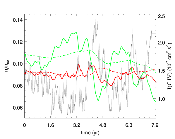
Figure 4: Simulations of Civ/C (green) and Nv/N (red) versus time for one lightcurve in the sample. The solid lines are for a density $n_{\scriptscriptstyle H}=10^{3.5}$ and the dashed lines are for $n_{\scriptscriptstyle H}=10^{2.5}$. The black line is the ionization rate per particle for C iv and is propotional to the simulated lightcurve for this example.

To determine an upper limit on the electron number density, we simulate the time-dependent changes in column densities of C iv and N v and compare them with the limits imposed by the observed differences between the STIS and COS data (see Table LABEL:line_data). For each given $n_{e}$, we track the fractional change in $N$(C iv) and $N$(N v) for all 935 simulated lightcurves in each of the seven troughs for which we have an initial photoionization solution. In Fig. 4, simulations for C iv and N v for two different electron number densities are shown for one of the simulated lightcurves with $t=0$ corresponding to the STIS epoch and $t\simeq 8$ yr corresponding to the COS epoch. From the simulations, histograms of the fraction of simulations versus the predicted change in column density are produced for each ion in each trough. We choose the upper limit on $n_{e}$ as the lowest density for which more than 99% of the lightcurves predict changes greater than those suggested by the data. Figure 5 shows an example of the resulting histograms, and Table LABEL:table:densities lists the results for each trough and ion.

Of components T1–T7, only T1 and T2 show a significant change in column densities. C iv is saturated in trough T1 and shows no significant change, but N v shows $>3\sigma$ changes in residual intensity for both components of the doublet. In trough T2, change is observed for C iv, while no change is observed for N v. Since these two components have responded to continuum changes, we can put a lower limit on $n_{e}$ and thereby, an upper limit on the distance. We do this by finding the highest density for which more than 99% of the lightcurves predict changes smaller than those suggested by the data. With distances $\raisebox{-2.15277pt}{$\;\stackrel{{\scriptstyle<}}{{\sim}}\;$}2.1$ kpc, these absorbers are within the confines of the host galaxy. We are also able to put an upper limit on $n_{e}$ using the same method. We note that our simulations for trough T1 predict changes that are smaller than that measured for both high and low densities. This is because the ionization parameter is near the value producing the highest N v fractional abundance ($U_{H}=10^{-1.5}$). As we increase $n_{e}$ from $10$ cm^-3 to $10^{4}$ cm^-3, the ionization state of the gas at the COS epoch increases. For $n_{e}\raisebox{-2.15277pt}{$\;\stackrel{{\scriptstyle<}}{{\sim}}\;$}100$ cm^-3, the change in $n$(N v) between STIS and COS epochs increases with increasing density. However, for $n_{e}\raisebox{-2.15277pt}{$\;\stackrel{{\scriptstyle>}}{{\sim}}\;$}100$ cm^-3, the N v column density decreases as the ionization of the gas becomes higher than than that producing the highest fractional abundance of N v. At densities of $n_{e}\simeq 10^{4}$ cm^-3, the lower ionization state at the time of the STIS observation and the higher ionization state at the time of the COS observations produce approximately the same amount of N v, and it therefore appears as if there is no change between epochs. For even higher densities, simulations predict a decrease in $n$(N v) between the STIS and COS epochs.

Figure 5: Determining the upper limit for $n_{\scriptscriptstyle H}$ of the absorber. This example shows the results for trough T2, based on the C iv column density measurements. For each of the 935 simulated light curves (see section 5), we explicitly solve the time-dependent photoionization equations and calculate the expected ratio of C iv column density over a time period equal to the differences between the STIS and COS epochs. Each panel represents the fractional solution distribution of $N$(C iv)${}_{COS}/N$(C iv)_STIS for a given $\log(n_{\scriptscriptstyle H})$ (cm^-3), which increases in the panels from left to right and top to bottom. The vertical dashed lines show the positive and negative 1$\sigma$ errors on the measured value. We determine an $n_{\scriptscriptstyle H}$ upper limit by increasing $n_{\scriptscriptstyle H}$ until more than 99% of the calculated $N$(C iv)${}_{COS}/N$(C iv)_STIS are outside the error bars. In this example, we find $n_{\scriptscriptstyle H}<10^{3.2}$ cm^-3.

Table 8: density and distance limits from simulations

Trough	$v$	log $n_{e}$(Civ)	log $n_{e}$(Nv)	$R_{99}$	$R_{90}$
	(km s-1)	(cm-3)	(cm-3)	(pc)	(pc)
T1	-405	$\cdots$	1.1–4.2	60–2100	80–1500
T2	-310	1.1–3.2	$<$4.2	160–1830	370–1460
T3	-240	$<$3.2	$<$3.9	$>$130	$>$290
T4	-70	$<$3.1	$<$3.4	$>$130	$>$290
T5	-15	$<$3.6	$\cdots$	$>$130	$>$260
T6	+45	$<$2.8	$<$3.2	$>$150	$>$370
T7	+125	$<$2.5	$\cdots$	$>$130	$>$290

We use the upper limits placed on the hydrogen number density $n_{\scriptscriptstyle H}$ (recall that $n_{\scriptscriptstyle H}\simeq n_{e}/1.2$ in highly ionized plasma) to determine lower limits on the distance to the absorber from the ionizing source via the ionization parameter (Equation 5). These are given in Table LABEL:table:densities, where $R_{99}$ and $R_{90}$ are the distances determined by requiring that 99% and 90% of the lightcurves, respectively, give results inconsistent with the differences in measured values. Except for component T1, these distances are determined using the $n_{e}$ derived from C iv since they give the smallest upper limit consistent with both the C iv and N v simulations. The rate of ionizing photons striking the gas is determined by fitting our SED to the 1175Å flux from STIS data given in Paper VI. We find $Q_{H}=5.03\times 10^{54}$ s^-1.

6 Discussion

We were able to put conservative lower limits on the distance to the absorber of 100–200 pc from the ionizing source for all the UV components using the fact that the column densities of C iv and N v showed little or no variation between the STIS and COS epochs despite a large change in ionizing flux. Since the lightcurve for Mrk 509 was not densely monitored between the epochs, we used Monte Carlo simulated lightcurves to statistically determine the distance limits.

The limits on the distance computed using timescale arguments (see Section 4) are similar to and bracket those we found statistically. For the lightcurve that increased just after the STIS epoch, the distance limits are 2.0 to 3.2 times larger than our 99% simulation based limits. For the lightcurve that increased just before the 100 days monitoring before the COS epoch, the distance limits are 1.6 to 2.6 times smaller than our 99% simulation based limits. Using the second lightcurve in the time-dependent ionization equations and requiring changes in ionic column density to be smaller than the 1-$\sigma$ errors given in Table 2 yields distances that are similar to our 90% simulation based limits and within a factor of 2 larger than our 99% simulation based limits for all troughs except T6 (factor of $\sim 3$ larger).

Our distance results are consistent with those derived for the simultaneous X-ray absorber data. In Paper III, five discrete ionization components were identified in the XMM-Newton spectrum of Mrk 509, named A, B, C, D, and E. Our analysis of the lack of spectral variability of these X-ray components during our campaign combined with variations seen in comparison with archival data (Paper VIII) showed that component C has a distance of $>$70 pc, component D is between 5 and 33 pc, and component E has a distance between 5 and 21–400 pc, depending upon modeling details. For the lowest ionization components, A and B, we were not able to establish any significant limits on the gas density or the distance. These low-ionization components, however, are closely associated with the UV components, so the bounds on distance that we establish in this paper completes our overall picture of the outflow in Mrk 509.

Based on the 100–200 pc lower limit for all the UV components, this absorber cannot be connected with an accretion disc wind. The outflow might have originated from the disc, but based on simple ballistic kinematics, such an event had to occur at least 300,000 years ago in the rest frame of the source.

Phillips et al. (1983) found extended emission in an area 6.6 kpc in diameter centered on the nucleus of Mrk 509. The radial velocities they measured for their high-ionization component correspond to the velocities for our troughs T2–T5, indicating that we may be seeing the same outflow. They also find a low-ionization component with line intensity ratios similar to Galactic H ii regions and velocities corresponding to our troughs T3–T7. If we are seeing the same outflow in absorption features as Phillips et al. (1983) saw in emission features, the distance to the absorbers is $\raisebox{-2.15277pt}{$\;\stackrel{{\scriptstyle>}}{{\sim}}\;$}3$ kpc (assuming a conical outlflow with an opening angle of $\raisebox{-2.15277pt}{$\;\stackrel{{\scriptstyle<}}{{\sim}}\;$}45^{\circ}$), putting them on scale with galactic winds (Veilleux et al. 2005).

Appendix A Behavior of the Time-dependent Photoionization Equations

As an illustrative example we look at the simple case of hydrogen. We are interested in the changes of neutral hydrogen in response to changes in ionizing flux. From equation (6) we obtain

$$\frac{dn_{\scriptscriptstyle H0}}{dt}=-n_{\scriptscriptstyle H0}I_{H0}+n_{\scriptscriptstyle H^{+}}R_{H0}.$$ (11)

Let us assume that we start from a steady state ionization equilibrium (Equation 9) with $I_{H0}=I_{0}$ , and that at $t=0$ the absorber experiences an instantaneous flux change: $I_{H0}(t>0)=I_{0}(1+f)$, where $f$ can be either positive or negative. We therefore obtain

$$\frac{dn_{\scriptscriptstyle H0}}{dt}=-(1+f)n_{\scriptscriptstyle H0}I_{0}+n_{\scriptscriptstyle H^{+}}R_{H0}$$ (12)

Assuming $n_{\scriptscriptstyle H^{+}}/n_{\scriptscriptstyle H0}\gg 1$ (as is typical for AGN outflow material), for an order of magnitude increase or decrease in flux, $n_{\scriptscriptstyle H^{+}}$ stays constant to a high degree, and therefore the right most term in equation (12) can be treated as constant. Under these assumptions there is a simple analytical solution for equation (12):

$$n_{\scriptscriptstyle H0}(t)=n_{\scriptscriptstyle H0}(0)\frac{1+fe^{-(1+f)I_{0}t}}{1+f}$$ (13)

This solution satisfies the differential equation as well as the two boundary conditions: $n_{\scriptscriptstyle H0}(t=0)=n_{\scriptscriptstyle H0}(0)$ and $n_{\scriptscriptstyle H0}(t=\infty)=n_{\scriptscriptstyle H0}(0)/(1+f)$, where the latter condition stems from the new steady state reached with flux level $I_{0}(1+f)$ (see Equation 9) Several properties of this solution are worth mentioning:

1. If we start from an ionization equilibrium, the timescale for changes in $n_{\scriptscriptstyle H0}(t)$ is

   $$[(1+f)I_{0}]^{-1}=[(1+f)\alpha_{\scriptscriptstyle H^{+}}n_{e}(n_{\scriptscriptstyle H^{+}}/n_{\scriptscriptstyle H0})_{t=0}]^{-1},$$ (14)

   which is inversely proportional to $n_{e}$. This is the timescale for 63% (1-$e^{-1}$) of the total $\Delta n_{\scriptscriptstyle H0}\equiv n_{\scriptscriptstyle H0}(0)-n_{\scriptscriptstyle H0}(\infty)$ change to occur. For $|f|\ll 1$, this timescale is approximately equal to that given by Equation 10.

2. For $f\gg 1$ the timescale for changes in $n_{\scriptscriptstyle H0}(t)$ is roughly given by $(I_{0}f)^{-1}$.

3. For a situation where $I_{H0}(t>t_{0})$ drops instantaneously back to $I_{0}$ we obtain two interesting limits:
   a) when $t_{0}\gg[(1+f)I_{0}]^{-1}$, $n_{\scriptscriptstyle H0}(t_{0})=n_{\scriptscriptstyle H0}(0)/(1+f)$, i.e., ionization equilibrium has been reached.
   b) when $t_{0}\ll[(1+f)I_{0}]^{-1}$, $n_{\scriptscriptstyle H0}(t_{0})=n_{\scriptscriptstyle H0}(0)(1-fI_{0}t_{0})$, which represent a damping in the maximum variation of $n_{\scriptscriptstyle H0}(t)$ that is inversely proportional to $n_{e}$ for a given $t_{0}$

The above three properties give insight to more physically interesting scenarios such as the ionization behavior of the absorber to abrupt cyclical changes in ionizing flux (see Figure 6).

Assuming $I_{H0}(t<0)=I_{0}$ and that $n_{e}$ is roughly constant at all times, we start with an ionization equilibrium $(n_{\scriptscriptstyle H^{+}}/n_{\scriptscriptstyle H0})_{t<0}=(I_{H0}/R_{H0})_{t<0}$. Following the three points above we expect that for $t_{0}\gg[(1+f)\alpha_{\scriptscriptstyle H^{+}}n_{e}(n_{\scriptscriptstyle H^{+}}/n_{\scriptscriptstyle H0})_{t=0}]^{-1}$ the absorber will quickly oscillate between the equilibria values: $n_{\scriptscriptstyle H0}=n_{\scriptscriptstyle H0}(0)/(1+f)$ and $n_{\scriptscriptstyle H0}(0)$. That is, in this limit the plasma has no memory for the history of ionizing flux changes and $n_{\scriptscriptstyle H0}$ closely follows the current value of $I_{H0}$. The situation is different for $t_{0}\ll[(1+f)\alpha_{\scriptscriptstyle H^{+}}n_{e}(n_{\scriptscriptstyle H^{+}}/n_{\scriptscriptstyle H0})_{t=0}]^{-1}$. Initially, each $t_{0}$ period of enhanced flux decreases $n_{\scriptscriptstyle H0}$ by a factor $fI_{0}t_{0}$, where $I_{0}t_{0}\ll 1$ by definition. After many cycles ($N\gg(I_{0}t_{0})^{-1}$) a pseudo equilibrium is reached where $n_{\scriptscriptstyle H0}=n_{\scriptscriptstyle H0}(0)/(1+f/2)$. In this case the plasma has a strong memory for the history of ionizing flux changes and the psuedo equilibrium depends on the average ionizing flux over $\Delta t\sim I_{0}^{-1}$.

For elements other than hydrogen, it is not possible to obtain useful analytical solutions for equation set (6). However the qualitative behavior is quite similar.

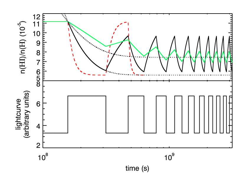
Figure 6: In the upper panel, simulations of the fraction of H inHi are plotted for a periodic step function light-curve with $\Delta t=1.6\times 10^{8}$ s (shown in the lower panel). The hydrogen number density of the thick black line was chosen to give a recombination timescale equal to half the period of the lightcurve. The red dashed line has a timescale that is 4 times shorter, and the green line has a timescale that is 4 times longer. The dotted black lines are analytic solutions for a flux change f=1 (lower line) and f=0.5 (upper line).

References

- Arav et al. (2001) Arav, N., de Kool, M., Korista, K. T., et al. 2001, ApJ, 561, 118
- Arav et al. (2005) Arav, N., Kaastra, J., Kriss, G. A., et al. 2005, ApJ, 620, 665
- Arav et al. (2002) Arav, N., Korista, K. T., & de Kool, M. 2002, ApJ, 566, 699
- Arav et al. (1999) Arav, N., Korista, K. T., de Kool, M., Junkkarinen, V. T., & Begelman, M. C. 1999, ApJ, 516, 27
- Bottorff et al. (2000) Bottorff, M. C., Korista, K. T., & Shlosman, I. 2000, ApJ, 537, 134
- Collier & Peterson (2001) Collier, S. & Peterson, B. M. 2001, ApJ, 555, 775
- Crenshaw et al. (2003) Crenshaw, D. M., Kraemer, S. B., & George, I. M. 2003, ARA&A, 41, 117
- Crenshaw et al. (2000) Crenshaw, D. M., Kraemer, S. B., Hutchings, J. B., et al. 2000, ApJ, 545, L27
- de Kool et al. (2001) de Kool, M., Arav, N., Becker, R. H., et al. 2001, ApJ, 548, 609
- Detmers et al. (2011) Detmers, R. G., Kaastra, J. S., Steenbrugge, K. C., et al. 2011, A&A, 534, A38
- Dunn et al. (2010a) Dunn, J. P., Bautista, M., Arav, N., et al. 2010a, ApJ, 709, 611
- Dunn et al. (2010b) Dunn, J. P., Crenshaw, D. M., Kraemer, S. B., & Trippe, M. L. 2010b, ApJ, 713, 900
- Dunn et al. (2006) Dunn, J. P., Jackson, B., Deo, R. P., et al. 2006, PASP, 118, 572
- Edmonds et al. (2011) Edmonds, D., Borguet, B., Arav, N., et al. 2011, ApJ, 739, 7
- Ferland et al. (1998) Ferland, G. J., Korista, K. T., Verner, D. A., et al. 1998, PASP, 110, 761
- Gabel et al. (2005) Gabel, J. R., Kraemer, S. B., Crenshaw, D. M., et al. 2005, ApJ, 631, 741
- Hamann et al. (1997) Hamann, F., Barlow, T. A., Junkkarinen, V., & Burbidge, E. M. 1997, ApJ, 478, 80
- Hamann et al. (2001) Hamann, F. W., Barlow, T. A., Chaffee, F. C., Foltz, C. B., & Weymann, R. J. 2001, ApJ, 550, 142
- Horne et al. (2004) Horne, K., Peterson, B. M., Collier, S. J., & Netzer, H. 2004, PASP, 116, 465
- Ishibashi & Courvoisier (2009) Ishibashi, W. & Courvoisier, T. J.-L. 2009, A&A, 504, 61
- Kaastra et al. (2012) Kaastra, J. S., Detmers, R. G., Mehdipour, M., et al. 2012, A&A, 539, A117
- Kaastra et al. (2011) Kaastra, J. S., Petrucci, P.-O., Cappi, M., et al. 2011, A&A, 534, A36
- Korista et al. (2008) Korista, K. T., Bautista, M. A., Arav, N., et al. 2008, ApJ, 688, 108
- Kraemer et al. (2003) Kraemer, S. B., Crenshaw, D. M., Yaqoob, T., et al. 2003, ApJ, 582, 125
- Kriss et al. (2011) Kriss, G. A., Arav, N., Kaastra, J. S., et al. 2011, A&A, 534, A41
- Kriss et al. (2000) Kriss, G. A., Peterson, B. M., Crenshaw, D. M., & Zheng, W. 2000, ApJ, 535, 58
- Krolik & Kriss (1995) Krolik, J. H. & Kriss, G. A. 1995, ApJ, 447, 512
- Lodders & Palme (2009) Lodders, K. & Palme, H. 2009, Meteoritics and Planetary Science Supplement, 72, 5154
- McHardy et al. (2006) McHardy, I. M., Koerding, E., Knigge, C., Uttley, P., & Fender, R. P. 2006, Nature, 444, 730
- Mehdipour et al. (2011) Mehdipour, M., Branduardi-Raymont, G., Kaastra, J. S., et al. 2011, A&A, 534, A39
- Moe et al. (2009) Moe, M., Arav, N., Bautista, M. A., & Korista, K. T. 2009, ApJ, 706, 525
- Netzer (2008) Netzer, H. 2008, New A Rev., 52, 257
- Nicastro et al. (1999) Nicastro, F., Fiore, F., Perola, G. C., & Elvis, M. 1999, ApJ, 512, 184
- Osterbrock & Ferland (2006) Osterbrock, D. E. & Ferland, G. J. 2006, Astrophysics of gaseous nebulae and active galactic nuclei
- Peterson et al. (1998) Peterson, B. M., Wanders, I., Horne, K., et al. 1998, PASP, 110, 660
- Phillips et al. (1983) Phillips, M. M., Baldwin, J. A., Atwood, B., & Carswell, R. F. 1983, ApJ, 274, 558
- Rodriguez-Pascual et al. (1997) Rodriguez-Pascual, P. M., Alloin, D., Clavel, J., et al. 1997, ApJS, 110, 9
- Steenbrugge et al. (2009) Steenbrugge, K. C., Fenovčík, M., Kaastra, J. S., Costantini, E., & Verbunt, F. 2009, A&A, 496, 107
- Steenbrugge et al. (2011) Steenbrugge, K. C., Kaastra, J. S., Detmers, R. G., et al. 2011, A&A, 534, A42
- Uttley et al. (2003) Uttley, P., Fruscione, A., McHardy, I., & Lamer, G. 2003, ApJ, 595, 656
- Veilleux et al. (2005) Veilleux, S., Cecil, G., & Bland-Hawthorn, J. 2005, ARA&A, 43, 769
- White & Peterson (1994) White, R. J. & Peterson, B. M. 1994, PASP, 106, 879