Controllable steep dispersion with gain in a four-level N-scheme with four-wave mixing

Abstract

We present a theoretical analysis of the propagation of light pulses through a medium of four-level atoms, with two strong pump fields and a weak signal field in an $N$-scheme arrangement. We show that the generation of four-wave mixing has a profound effect on the signal field group velocity and absorption, allowing the signal field propagation to be tuned from superluminal to slow light regimes with amplification.

I Introduction

Precise rotation sensors are critical components for stabilization, navigation, and targeting applications. At the moment, the most sensitive commercial devices are optical gyroscopes based on the Sagnac effect sagnac (1). Such a device consists of a ring interferometer with two counter-propagating light waves, as shown in Fig. 1. The rotation of such an interferometer results in a phase difference between the two optical fields proportional to the magnitude of the rotational angular velocity $\vec{\Omega}$:

$$\Delta\phi=\frac{4\pi\omega}{c^{2}}\vec{A}\cdot\vec{\Omega},$$ (1)

where $\omega$ is the light angular frequency, $c$ is the speed of light, and $\vec{A}$ is the area of the optical loop. Most successful realizations to date are fiber-optics gyroscopes, in which the interferometer ring is formed by a loop of an optical fiber. The sensitivity of such an interferometer is usually boosted by using a large number $N$ of loops that increase the effective area in Eq. (1) by a factor of $N$. The Sagnac phase shift can then be measured directly from the interference of the two counter-propagating waves at the output, or by monitoring the resulting frequency difference between corresponding counter-propagating modes of the interferometer cavity. In either case, the reciprocity of light propagation dramatically reduces effects of environmental factors (temperature, vibrations, etc.), and ensures high reliability. As a result, the sensitivity of state-of-the-art compact fiber-optic gyroscopes has reached the shot-noise-limited value of $10^{-7}$–$10^{-8}~{}\mathrm{rad/s/\sqrt{Hz}}$ optgyrosens (2), while large-area laser gyroscopes have achieved even greater sensitivities, on the order of $10^{-10}~{}\mathrm{rad/s/\sqrt{Hz}}$ lasergyro (3).

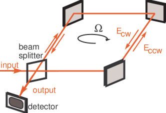
Figure 1: Generic schematic of a generic optical gyroscope based on the Sagnac effect.

Similar sensitivity has been also achieved with matter-based Sagnac interferometers. In this case, the rotation-induced phase equation may be written as

$$\Delta\phi=\frac{4\pi}{\lambda_{\rm dB}{v}}\vec{A}\cdot\vec{\Omega},$$ (2)

where ${v}$ and $\lambda_{\rm dB}=2\pi\hbar/(mv)$ represent the average velocity and the de Broglie wavelength of the massive particles, respectively. Here, the advantage gained by the use of massive particles ($mc^{2}\gg\hbar\omega$) is offset by the much smaller effective area compared to fiber-optics devices, resulting in similar performance kasevich00 (4).

Recent demonstrations of slow light pulse propagation in coherent optical media stirred active debate on the possibility of using slow-light pulses to enhance the Sagnac effect. It was quickly established that neither large positive (“slow light”) nor negative (“fast light”) dispersion has a direct influence on the magnitude of the Sagnac phase shift in Eq. (1) malykin00 (5).

Nevertheless, it still seems to be possible to take advantage of a large group index to enhance gyroscopic performance. For example, the output signal of a rotating interferometer with a highly dispersive slow-light medium can be enhanced by its differential response to opposite Sagnac phase shifts of two counter-propagating light waves PengLiXu07 (6). A modest factor-of-$2.5$ enhancement of the observed phase difference has been recently demonstrated in a slow light fiber ring Yuan10 (7), and a more significant enhancement (up to a factor of 200) is predicted in certain coupled resonator structures PengLiXu07 (6).

Even more dramatic improvements are predicted for the measurement of the Sagnac-effect-induced mode splitting in an active ring cavity with strong negative dispersion shahriarPRA07 (8). Calculations have shown that the resulting frequency difference between two counter-propagating modes is inversely proportional to the group index, and thus nominally diverges for $n_{g}=0$ (i.e., for $n\simeq-\omega\frac{\partial n}{\partial\omega}$) shahriarPRA07 (8, 9). While this divergence disappears after correcting for higher-order nonlinear effects, a $10^{6}$ improvement in gyroscope sensitivity should still be possible.

The current status of these debates shows that while strong positive or negative optical dispersion may indeed be capable of dramatic improvements in optical gyroscope performance, there is no clear winning approach. Thus, an atomic system that can be easily reconfigured to exhibit either strong positive or strong negative dispersion is an ideal candidate for the development of such a new generation of advanced optical gyroscopes. In the last decade, controllable manipulations of the group velocity of light have been demonstrated in a wide range of systems Boyd2002 (10, 11). Nonetheless, atomic systems with long-lived spin coherences still provide the highest values of group index for both slow and fast light regimes Akulshin2010 (12). In such atomic systems, the group velocity for a probe optical field can be widely tuned by adjusting parameters of a strong control field that provides strong coupling of the probe optical field to a collective atomic spin state lukin03rmp (13).

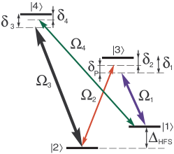
Figure 2: Schematic for four optical fields interacting with four-level atoms in an N-configuration.

An ideal test system for the development of a new type of optical gyroscope with improved rotational sensitivity should have a dispersion that can be continuously controlled in the widest possible range—from the highest positive group index to the highest negative group index—with minimal changes in the experimental arrangement. While several interaction schemes are capable of such wide tunability akulshin03 (14, 15), a so-called N-scheme has recently emerged as a promising candidate harris98 (16, 17, 18, 19, 20). A possible realization of an N-scheme is formed by three optical fields interacting with four-level atoms in the arrangement shown in Fig. 2. In the absence of the control field, the two resonant optical fields $\Omega_{1,2}$ form a regular $\Lambda$ system exhibiting EIT and slow light lukin03rmp (13). The interaction of the atoms with the second strong control field $\Omega_{3}$ splits this single EIT peak into two, separated by a narrow enhanced-absorption peak. This spectral region exhibits a fast-light effect, desired for gyroscope performance enhancement. However, this fast-light regime cannot be directly utilized in the proposed active enhanced-sensitivity optical gyroscope due to its unavoidable high optical losses.

In this manuscript, we provide an extended treatment of the four-level N-scheme that includes the possibility of four-wave mixing (FWM) by allowing optical transitions (and spontaneous decay) between states $|4\rangle$ and $|1\rangle$. The associated FWM gain modifies the transmission of the probe field FleischhakerPRA08 (21, 22), and provides a smooth switch between slow- and fast-light regimes by varying the strength of one of the pump fields ($\Omega_{3}$).

II Slow and Fast light in a four-level N-scheme

The evolution of a four-level N-system, shown in Fig. 2, can be described under the rotating-wave approximation by the following Hamiltonian:

$$\frac{\hat{H}}{i\hbar}=\left(\begin{array}[]{cccc}0&0&-\frac{1}{2}e^{-i\phi_{1}}\Omega_{1}&-\frac{1}{2}e^{-i\phi_{4}}\Omega_{4}\\ 0&-\delta_{1}+\delta_{2}&-\frac{1}{2}e^{-i\phi_{2}}\Omega_{2}&-\frac{1}{2}e^{-i\phi_{3}}\Omega_{3}\\ -\frac{1}{2}e^{i\phi_{1}}\Omega_{1}&-\frac{1}{2}e^{i\phi_{2}}\Omega_{2}&-\delta_{1}&0\\ -\frac{1}{2}e^{i\phi_{4}}\Omega_{4}&-\frac{1}{2}e^{i\phi_{3}}\Omega_{3}&0&-\delta_{1}+\delta_{2}-\delta_{3}\end{array}\right),$$ (3)

where $\Omega_{i}$ and $\phi_{i}$ are the Rabi frequencies and phases of the corresponding optical fields, respectively, and $\delta_{i}$ are their detunings from the corresponding optical transitions, as shown in Fig. 2. Here we have assumed the four-photon resonance condition $-\delta_{1}+\delta_{2}-\delta_{3}+\delta_{4}=0$, as well as the phase-matching condition on the optical wavenumbers $k_{i}$, $-k_{1}+k_{2}-k_{3}+k_{4}=0$, which results in the elimination of the explicit time and space dependence from the Hamiltonian mahmoudiPRA06 (23). The four-photon resonance condition is automatically satisfied in the situation that we will primarily consider, in which the Stokes field $\Omega_{4}$ is spontaneously generated.

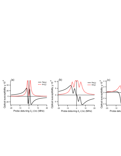
Figure 3: Real and imaginary parts of the probe-field susceptibility for various interaction configurations: (a) only one control field $\Omega_{1}=(2\pi)\,3$ MHz is on (standard EIT regime); (b) both control fields $\Omega_{1}=(2\pi)\,3$ MHz and $\Omega_{3}=(2\pi)\,6$ MHz are present, but no radiative transition between states $|4\rangle$ and $|1\rangle$ is allowed (standard N-scheme); (c) both control fields $\Omega_{1}=(2\pi)\,3$ MHz and $\Omega_{3}=(2\pi)\,6$ MHz are present, and both excited states have equal decay rates into each of the ground states. For all graphs the excited state decay rates are $\gamma_{3}=\gamma_{4}=(2\pi)\,3$ MHz, the ground-state relaxation rate is $(2\pi)\,0.01$ MHz, we assume equal branching ratios for all optical transitions, and both pump fields are resonant with corresponding optical transitions.

The ability to control the dispersion of the probe field $\Omega_{2}$ by adjusting the intensities of two strong control fields $\Omega_{1}$ and $\Omega_{3}$ is illustrated in Fig. 3, obtained by numerically solving the evolution equations obtained from the above Hamiltonian for the steady-state condition. Figure 3(a) shows a traditional EIT regime, with a moderately strong first control field $\Omega_{1}=(2\pi)\,3$ MHz and the second control field $\Omega_{3}$ turned off. As expected, we observe a dip in the absorption spectrum (dashed line) and steep, positive, linear dispersion of the refractive index (solid line) near zero two-photon detuning $\delta_{P}=\delta_{2}-\delta_{1}=0$, between two absorption peaks corresponding to the Autler-Townes splitting of the excited state by the strong control field. Figure 3(b) depicts the situation in which the atoms interact with both strong control fields $\Omega_{1}$ and $\Omega_{3}$ in a standard N-configuration, in which optical transition from state $|4\rangle$ to $|1\rangle$ is not allowed by selection rules. In this case, the spectrum consists of four partially-resolved absorption resonances, which can be interpreted as unequal Autler-Townes splittings of the states $|2\rangle$ and $|3\rangle$ by the control fields of different intensities $\Omega_{1}=(2\pi)\,3$ MHz and $\Omega_{3}=(2\pi)\,6$ MHz. Even though there are several spectral regions in which steep anomalous dispersion is realized, all of them occur in conjunction with enhanced absorption.

Finally, Figure 3(c) shows that the situation is quite different if optical transitions are allowed from both excited states to each of the ground states. In this case, the four-wave mixing process in a double-$\Lambda$ system is possible, and it is enhanced through the long-lived spin coherence between states $|1\rangle$ and $|2\rangle$ lukin03rmp (13, 24, 22). As a result, a new optical Stokes field $\Omega_{4}$ is efficiently generated, and the probe-field spectrum consists of two antisymmetric Raman resonances, with gain regions at both positive and negative probe-field detunings. For properly chosen intensities of the two control fields, it is possible to adjust the frequency splitting and widths of these peaks to achieve a negatively-sloped refractive index for the probe field near the zero two-photon detuning $\delta_{P}=0$, while the its gain drops to zero between the two gain peaks. Thus, the probe field experiences minimal absorption or gain for frequencies near the two-photon resonance, which are the desired characteristics of an atomic medium for gyroscope enhancement.

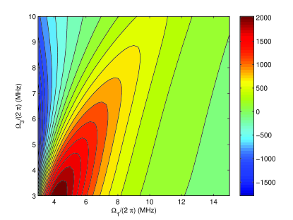
Figure 4: Optimization of the probe-field group index $n_{g}$ on the two-photon resonance, as function of both control fields’ strengths. For this calculation, we assumed $1$ cm-long atomic medium of $10^{9}$ cm Rb density; the rest of the experimental parameters are the same as in Fig. 3. Zero probe-field absorption is predicted for the shown range of control fields’ Rabi frequencies.

From this picture, it is clear that optimization of the control field intensities allows for smooth tuning of the probe field’s dispersion from slow to fast light regimes by changing the frequency shift and shape of the Raman peaks. To find the optimal operational parameters numerically, we compute the spectrum of the probe field $\Omega_{2}$ for the range of the control fields’ Rabi frequencies and calculate dispersion at the zero two-photon resonance. The results are shown in Fig. 4. One can see that depending on the ratio between two control fields, the probe experiences either slow light (when the two gain peaks for positive and negative two-photon detuning are not resolved and form a single gain peak), or fast light (when the two peak are farther apart, forming a distinct dip between them). When both fields are very strong, the Raman resonances are shifted too far from the origin, leading to flat dispersion. From this analysis we have identified $\Omega_{1}=(2\pi)\,3$ MHz and $\Omega_{3}=(2\pi)\,6$ MHz as suitable values for producing the desired lossless fast-light behavior.

Under the four-wave mixing condition, the spontaneously generated Stokes field $\Omega_{4}$ experiences strong gain, and thus its intensity increases as it propagates through the medium. Moreover, its presence has a strong effect on the probe field amplitude due to their mutual coupling through the atomic spin coherence, even though both probe and Stokes fields remain significantly weaker than either control field. In Fig. 5, we plot the real and imaginary parts of optical polarizations for both the probe (top) and Stokes (bottom) fields, under conditions corresponding to different points along the optical path through the atomic medium. The left column represents the entrance of the vapor cell, where only the probe field is present, and $\Omega_{4}=0$ since it is not yet generated. Under these conditions, $\Omega_{4}$ experiences strong gain, which leads to its spontaneous generation. The Stokes field is generated at the frequency that satisfies the four-photon resonance condition—any variation in the probe two-photon detuning $\delta_{P}=\delta_{2}-\delta_{1}$ is matched by the corresponding change in the Stokes field two-photon detuning $\delta_{S}=\delta_{4}-\delta_{3}=-\delta_{P}$.

As the unattenuated probe light and generated Stokes field propagate along the cell, the increasing strength of $\Omega_{4}$ starts affecting the propagation of the probe field through the FWM coupling. In particular, the negatively-sloped refractive index is somewhat flattened out, due to appearance of a small amount of gain [Fig. 5(c)]. Farther along the cell, the probe field experiences stronger gain, but the dispersion switches to non-anomalous, associated with slow-light propagation regime. The observed behavior indicates the the amplitude of the Stokes field offers an additional control mechanism of the group index through, for example, the optical depth of the atomic ensemble. At the same time, the four-wave mixing process produces higher gain for the probe field at the output, and thus allows for compensation of unavoidable optical losses when operating inside a cavity.

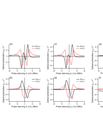
Figure 5: Top row: Real and imaginary parts of atomic polarization $\rho_{3,2}$, proportional to the refractive index and absorption for the probe field $\Omega_{2}$ for for various strengths of the Stokes field. Bottom row: Same for real and imaginary parts of atomic polarization $\rho_{4,1}$ for the Stokes field $\Omega_{4}$. Pump fields are $\Omega_{1}=(2\pi)\,3$ MHz and $\Omega_{3}=(2\pi)\,6$ MHz.

III Analytical solution

The results presented above have been obtained by numerical solution of the propagation equations for all four optical fields using interaction Hamiltonian, described by Eq. (3) without making any additional assumptions about the parameters of the system. However, with a few reasonable approximations, we also can find an analytical solution for time-dependent weak optical fields $\Omega_{2}$ and $\Omega_{4}$ and strong cw optical fields $\Omega_{1}$ and $\Omega_{3}$. In this case we can assume a linear response of the atomic medium in response to both weak optical fields. The strong control fields determine the populations of the atomic levels and optical polarizations for the $|1\rangle\rightarrow|3\rangle$ and $|2\rangle\rightarrow|4\rangle$ transitions that are coupled with these fields. Thus, the corresponding density matrix elements can be calculated assuming only the interaction of the two strong fields with the atoms, which in the interaction scheme under consideration (Fig. 2) reduces to the simple case of two independent two-level systems, connected only through the decays of the excited states $|3\rangle$ and $|4\rangle$:

$$\dot{\rho}_{1,1} = \gamma_{31}\rho_{3,3}+\gamma_{41}\rho_{4,4}+\frac{1}{2}i\Omega_{1}(\rho_{3,1}-\rho_{1,3})$$ (4)

$$\dot{\rho}_{2,2} = \gamma_{32}\rho_{3,3}+\gamma_{42}\rho_{4,4}+\frac{1}{2}i\Omega_{2}(\rho_{4,2}-\rho_{2,4})$$ (5)

$$\dot{\rho}_{3,3} = -\gamma_{3}\rho_{3,3}-\frac{1}{2}i\Omega_{1}(\rho_{3,1}-\rho_{1,3})$$ (6)

$$\dot{\rho}_{4,4} = -\gamma_{4}\rho_{4,4}-\frac{1}{2}i\Omega_{2}(\rho_{4,2}-\rho_{2,4})$$ (7)

$$\dot{\rho}_{1,3} = -(\gamma_{3}/2+i\delta_{1})\rho_{1,3}-\frac{1}{2}i\Omega_{1}(\rho_{1,1}-\rho_{3,3})$$ (8)

$$\dot{\rho}_{2,4} = -(\gamma_{4}/2+i\delta_{3})\rho_{2,4}-\frac{1}{2}i\Omega_{3}(\rho_{2,2}-\rho_{4,4})$$ (9)

Here $\gamma_{3}=\gamma_{31}+\gamma_{32}$ and $\gamma_{4}=\gamma_{41}+\gamma_{42}$ are the population decay rates of the excited states. For simplicity, we have neglected the population decay rates from the two ground states, assuming that they are significantly smaller than the excited state decays and the strong optical fields’ Rabi frequencies. Comparison with the exact numerical solutions indicates that this is a good approximation.

Solving Eqs. (4-9) in the steady state and assuming equal branching ratios for the excited state decay channels ($\gamma_{31}=\gamma_{32}=\gamma_{3}/2$ and $\gamma_{41}=\gamma_{42}=\gamma_{4}/2$), we obtain the following expressions for atomic populations and optical coherences:

$$\left(\begin{array}[]{c}\rho_{1,1}^{(0)}\\ \rho_{2,2}^{(0)}\\ \rho_{3,3}^{(0)}\\ \rho_{4,4}^{(0)}\\ \rho_{1,3}^{(0)}\\ \rho_{2,4}^{(0)}\\ \end{array}\right)=\frac{1}{T}\left(\begin{array}[]{c}\Omega_{3}^{2}(4\delta_{1}^{2}+\Omega_{1}^{2}+\gamma_{3}^{2})\gamma_{4}\\ \Omega_{1}^{2}(4\delta_{3}^{2}+\Omega_{3}^{2}+\gamma_{4}^{2})\gamma_{3}\\ \Omega_{1}^{2}\Omega_{3}^{2}\gamma_{4}\\ \Omega_{1}^{2}\Omega_{3}^{2}\gamma_{3}\\ -\Omega_{1}\Omega_{3}^{2}\gamma_{4}(2\delta_{1}+i\gamma_{3})\\ -\Omega_{3}\Omega_{1}^{2}\gamma_{3}(2\delta_{3}+i\gamma_{4})\\ \end{array}\right),$$ (10)

where $T=2{\Omega_{3}}^{2}\gamma_{4}\left(2{\delta_{1}}^{2}+{\Omega_{1}}^{2}\right)+\gamma_{3}\gamma_{4}\left({\Omega_{3}}^{2}\gamma_{3}+{\Omega_{1}}^{2}\gamma_{4}\right)+2{\Omega_{1}}^{2}\gamma_{3}\left(2{\delta_{3}}^{2}+{\Omega_{3}}^{2}\right)$ is the common denominator. We make the additional approximation that the values of these density matrix elements do not change along the length of the cell. The validity of this approximation may be questioned, since, in fact, both strong fields will experience some absorption. Later, we will demonstrate that in the range of strong field intensities that produce the desired fast-light regime this absorption is not significant, and the non-depletion approximation is reasonable.

We are interested in calculating the propagation of the weak probe field $\Omega_{2}$, as well as in the possible generation of the four-wave mixing field $\Omega_{4}$ connecting the $|4\rangle$ and $|1\rangle$ transition, governed by the wave equation,

$$(-i\omega+c\partial_{z})\Omega_{2} = ig_{2}N\rho_{3,2},$$ (11)

$$(-i\omega+c\partial_{z})\Omega_{4} = ig_{4}N\rho_{4,1},$$ (12)

where $g_{2,4}$ are coupling coefficients for the corresponding optical transitions.

The remaining density matrix elements are described by the following equations:

$$\dot{\rho}_{1,2} = -\Gamma_{12}\rho_{1,2}+\frac{1}{2}i\Omega_{1}\rho_{3,2}-\frac{1}{2}i\Omega_{3}\rho_{1,4}-\frac{1}{2}i\Omega_{2}\rho_{1,3}^{(0)}+\frac{1}{2}i\Omega_{4}\rho_{4,2}^{(0)};$$ (13)

$$\dot{\rho}_{1,4} = -\Gamma_{14}\rho_{1,4}+\frac{1}{2}i\Omega_{1}\rho_{3,4}-\frac{1}{2}i\Omega_{3}\rho_{1,2}+\frac{1}{2}i\Omega_{4}(\rho_{4,4}^{(0)}-\rho_{1,1}^{(0)});$$ (14)

$$\dot{\rho}_{3,2} = -\Gamma_{32}\rho_{3,2}+\frac{1}{2}i\Omega_{1}\rho_{1,2}-\frac{1}{2}i\Omega_{3}\rho_{3,4}-\frac{1}{2}i\Omega_{2}(\rho_{3,3}^{(0)}-\rho_{2,2}^{(0)});$$ (15)

$$\dot{\rho}_{3,4} = -\Gamma_{34}\rho_{3,4}+\frac{1}{2}i\Omega_{1}\rho_{1,4}-\frac{1}{2}i\Omega_{3}\rho_{3,2}+\frac{1}{2}i\Omega_{2}\rho_{2,4}^{(0)}-\frac{1}{2}i\Omega_{4}\rho_{3,1}^{(0)};$$ (16)

where $\Gamma_{12}=i(\delta_{1}-\delta_{2})$, $\Gamma_{14}=\gamma_{4}/2+i(\delta_{1}-\delta_{2}+\delta_{3})$, $\Gamma_{32}=\gamma_{3}/2-i\delta_{2}$, and $\Gamma_{34}=(\gamma_{3}+\gamma_{4})/2+i(\delta_{3}-\delta_{2})$.

It is important to note that we assume that the detuning of this generated field is such that it always obeys the four-photon resonance condition $-\delta_{1}+\delta_{2}-\delta_{3}+\delta_{4}=0$. For example, if both strong fields are tuned to the atomic transition frequencies ($\delta_{1}=\delta_{3}=0$) and the probe field detuning $\delta_{2}$ is scanned, the detuning of the generated Stokes field changes in the opposite direction $\delta_{4}=-\delta_{2}$ to maintain the resonance.

Equations (13–16) can be compactly written as

$$\dot{\rho}_{\downarrow}=M\rho_{\downarrow}+B,$$ (17)

where vector $\rho_{\downarrow}$ consists of the four unknown density matrix elements $(\rho_{\downarrow})^{\mathrm{T}}=\{\rho_{1,2},\rho_{1,4},\rho_{3,2},\rho_{3,4}\}$, $M$ is a $4\times 4$ matrix:

$$M=\left(\begin{array}[]{cccc}i\delta_{2}&-i\Omega_{3}/2&i\Omega_{1}/2&0\\ -i\Omega_{3}/2&i\delta_{2}-\gamma_{4}/2&0&i\Omega_{1}/2\\ i\Omega_{1}/2&0&i\delta_{2}-\gamma_{3}/2&-i\Omega_{3}/2\\ 0&i\Omega_{1}/2&-i\Omega_{3}/2&i\delta_{2}-\gamma_{3}/2-\gamma_{4}/2\\ \end{array}\right),$$ (18)

and $B$ is defined as

$$B=\frac{1}{iT}\left(\begin{array}[]{c}\Omega_{1}\Omega_{3}(\Omega_{2}\Omega_{3}+\Omega_{1}\Omega_{4})\gamma_{3}\gamma_{4}\\ i{\Omega_{3}}^{2}\Omega_{4}\left({\Omega_{1}}^{2}\gamma_{3}-{\Omega_{1}}^{2}\gamma_{4}-\gamma_{3}^{2}\gamma_{4}\right)\\ i{\Omega_{1}}^{2}\Omega_{2}\left({\Omega_{3}}^{2}\gamma_{4}-{\Omega_{3}}^{2}\gamma_{3}-\gamma_{3}\gamma_{4}^{2}\right)\\ \Omega_{1}\Omega_{3}(\Omega_{1}\Omega_{2}+\Omega_{3}\Omega_{4})\gamma_{3}\gamma_{4}\\ \end{array}\right).$$ (19)

In this case the solution of Eq. (20) in the frequency domain is

$$\rho_{\downarrow}^{(1)}=-(M+i\omega\mathbf{I})^{-1}B,$$ (20)

where $\mathbf{I}$ is the identity matrix. Finally, the calculated expressions for the density matrix elements $\rho_{3,2}$ and $\rho_{1,4}$ in terms of the optical-field Rabi frequencies must be substituted into Eqs. (11,12) to obtain the propagation equations for the probe and Stokes field in a self-consistent form:

$$\partial_{z}\left(\begin{array}[]{c}\Omega_{2}\\ \Omega_{4}\\ \end{array}\right)=\frac{iNg}{c}M_{2}\left(\begin{array}[]{c}\Omega_{2}\\ \Omega_{4}\\ \end{array}\right),$$ (21)

where the matrix $M_{2}$ contains the information about atomic response, and we assume equal coupling coefficients $g_{2}=g_{4}=g$. The explicit form of the matrix $M_{2}$ consists of algebraic combinations of the Rabi frequencies and detunings of the strong optical fields and optical transition decay rates, but is omitted here for brevity.

The important consequence of the non-depletion approximation for the strong fields is that the right-hand side of Eq. (21) does not depend on position $z$, allowing a direct solution:

$$\left(\begin{array}[]{c}\Omega_{2}(\omega,z)\\ \Omega_{4}(\omega,z)\\ \end{array}\right) = e^{\frac{iNg}{c}M_{2}z}\left(\begin{array}[]{c}\Omega_{2}(\omega,0)\\ \Omega_{4}(\omega,0)\\ \end{array}\right)$$ (26)

$$\equiv \left(\begin{array}[]{cc}A(\omega,z)&B(\omega,z)\\ C(\omega,z)&D(\omega,z)\\ \end{array}\right)\left(\begin{array}[]{c}\Omega_{2}(\omega,0)\\ \Omega_{4}(\omega,0)\\ \end{array}\right).$$ (31)

Here $\Omega_{2,4}(0)$ are the Rabi frequencies corresponding to the input probe and Stokes fields. It is important to note that expanding the expressions for the coefficients $A$-$D$ forms in Taylor series up to the $\omega^{2}$ terms accurately captures the pulse propagation dynamics, but allows significant speed-up in the calculations. The results presented below were obtained in this approximation.

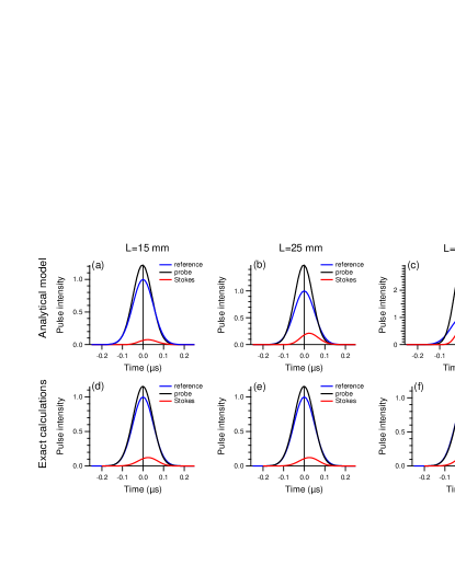
Figure 6: Comparison between exact solution (top) and approximate analytical calculations (bottom) of the signal pulse propagation through the cell of varying length.

Fourier transformation of this solution describes the propagation dynamics of signal/Stokes optical fields. Fig. 6 demonstrates the comparison between the exact numerical solutions obtained by calculating all time-dependent density matrix elements and propagation for all four optical fields, and the prediction of our simplified analytical theory for propagation of a 100-ns Gaussian probe pulse through an atomic medium with density $10^{9}~{}\mathrm{cm}^{-3}$. We observe that, for short lengths of the atomic medium (15 mm and 25 mm), the two methods provide similar solutions, predicting small gain and some advance for the probe optical field, as well as generation of the Stokes field in a slow-light regime. For the longer cell (50 mm), however, the analytical model significantly overestimates the gain in both probe and Stokes fields compared to the exact numerical solution that takes into the account the attenuation of both strong control fields associated population redistribution. Nevertheless, it is interesting to note that both models predict positive delay for the probe pulse for the longer cell, with similar delay time.

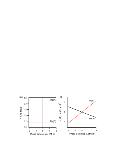
Figure 7: Coefficients $A$ and $B$ of the transfer matrix Eq. (26) for near-zero probe detuning $\delta_{2}$. The calculations are made for conditions identical to those of Fig. 6(a).

The analytical solution also provides useful intuition about the role of the generated Stokes field in the dynamics of the probe optical field. For example, Fig. 7 shows the real and imaginary parts of the coefficients $A$ and $B$ of the transfer matrix in Eq. (26) for a relatively short atomic medium ($L=1$ cm). The real part of these coefficients [Fig. 7(a)] illustrates that both input probe and Stokes fields directly contribute to the predicted amplification of the probe field after the cell, and have no spectral dependence near the resonance. The imaginary parts of the coefficients, shown in Fig. 7(b), represent the dispersive effect of the atomic medium. They are both nearly linear functions of frequency, with slopes of opposite sign. Also, for the chosen detunings, $\partial\text{Im}(B)/\partial\omega$, representing the Stokes field contribution to the dispersion, is approximately twice as steep as $\partial\text{Im}(A)/\partial\omega$. Thus, it is not surprising that for very weak Stokes fields (corresponding to low optical depth values) the dispersion is predominantly determined by the probe field propagation, and displays “fast light” regime. As the amplitude of the Stokes field increases, it adds up with the opposite phase to the output field, and, eventually, changes the sign of the dispersion. Under these conditions, the output probe field is delayed, as in the “slow light” regime.

IV Conclusions

In conclusion, we have analyzed the propagation of a weak resonant probe through a medium of four-level atoms in an N-scheme with allowed four-wave mixing generation, and found it to be a promising candidate for the realization of tunable “slow-to-fast” light with no absorption. This is particularly interesting for the experimental investigation of potential techniques for the enhancement of optical-gyroscope performance.

V Acknowledgments

The authors thank Frank Narducci and John Davis for useful discussions. This research was supported by Naval Air Warfare Center STTR program N68335-11-C-0428.

References

- (1) Sagnac, G. L’éther lumineux démontré par l’effet du vent relatif d’éther dans un interféromètre en rotation uniforme. Comptes rendus de l’Académie des Sciences 1913, 95, 708–710.
- (2) Lefevre, H.C., Application of the Sagnac Effect in the Interferometric Fiber-Optic Gyroscope, Optical Gyros and Their Application ; , 1999; pp 7:1–7:29.
- (3) Stedman, G.E.; Schreiber, K.U.; Bilger, H.R. On the detectability of the Lense–Thirring field from rotating laboratory masses using ring laser gyroscope interferometers. Class. Quantum Gravity 2003, 20 (13), 2527.
- (4) Gustavson, T.L.; Landragin, A.; Kasevich, M.A. Rotation sensing with a dual atom-interferometer Sagnac gyroscope. Class. Quantum Gravity 2000, 17 (12), 2385.
- (5) Malykin, G.B. The Sagnac effect: correct and incorrect explanations. Physics-Uspekhi 2000, 43 (12), 1229.
- (6) Peng, C.; Li, Z.; Xu, A. Optical gyroscope based on a coupled resonator with the all-optical analogous property of electromagnetically induced transparency. Opt. Express 2007, 15 (7), 3864–3875.
- (7) Zhang, Y.; Tian, H.; Zhang, X.; Wang, N.; Zhang, J.; Wu, H.; et al. Experimental evidence of enhanced rotation sensing in a slow-light structure. Opt. Lett. 2010, 35 (5), 691–693.
- (8) Shahriar, M.S.; Pati, G.S.; Tripathi, R.; Gopal, V.; Messall, M.; et al. Ultrahigh enhancement in absolute and relative rotation sensing using fast and slow light. Phys. Rev. A 2007, 75 (5), 053807.
- (9) Pati, G.S.; Salit, M.; Salit, K.; et al. Demonstration of displacement-measurement-sensitivity proportional to inverse group index of intra-cavity medium in a ring resonator. Opt. Commun. 2008, 281 (19), 4931–4935.
- (10) Boyd, R.W.; Gauthier, D.J.; Wolf, E. “Slow” and “fast” light. Progress in Optics In Vol. 43 0079-6638 doi: DOI: 10.1016/S0079-6638(02)80030-0 : , 2002 0079-6638 doi: DOI: 10.1016/S0079-6638(02)80030-0; pp 497–530.
- (11) Boyd, R.W.; Gauthier, D.J. Controlling the Velocity of Light Pulses. Science 2009, 326 (5956), 1074–1077.
- (12) Akulshin, A.M.; McLean, R.J. Fast light in atomic media. Journal of Optics 2010, 12 (10), 104001.
- (13) Lukin, M.D. Colloquium: Trapping and manipulating photon states in atomic ensembles. Rev. Mod. Phys. 2003, 75 (2), 457.
- (14) Akulshin, A.M.; Cimmino, A.; Sidorov, A.I.; Hannaford, P.; et al. Light propagation in an atomic medium with steep and sign-reversible dispersion. Phys. Rev. A 2003, 67 (1), 011801.
- (15) Mikhailov, E.E.; Sautenkov, V.A.; Novikova, I.; et al. Large negative and positive delay of optical pulses in coherently prepared dense Rb vapor with buffer gas. Phys. Rev. A 2004, 69 (6), 063808.
- (16) Harris, S.E.; Yamamoto, Y. Photon Switching by Quantum Interference. Phys. Rev. Lett. 1998, 81 (17), 3611.
- (17) Kang, H.; Hernandez, G.; Zhu, Y. Superluminal and slow light propagation in cold atoms. Phys. Rev. A 2004, 70 (1), 011801.
- (18) Yi, C.; Wei, X.G.; Ham, B.S. Optical properties of an N-type system in Doppler-broadened multilevel atomic media of the rubidium D2 line. J. Phys. B 2009, 42 (6), 065506.
- (19) Abi-Salloum, T.Y.; Snell, S.; Davis, J.P.; et al. Variations of dispersion and transparency in four level N-scheme atomic systems. Journal of Modern Optics 2011, 58 (21, SI), 2008–2014.
- (20) Abi-Salloum, T.Y.; Henry, B.; Davis, J.P.; et al. Resonances and excitation pathways in four-level N-scheme atomic systems. Phys. Rev. A 2010, 82 (1), 013834.
- (21) Fleischhaker, R.; Evers, J. Four-wave mixing enhanced white-light cavity. Phys. Rev. A 2008, 78 (Nov), 051802.
- (22) Glasser, R.T.; Vogl, U.; Lett, P.D., Stimulated generation of superluminal light pulses via four-wave mixing, arXiv:1204.0810, 2012.
- (23) Mahmoudi, M.; Evers, J. Light propagation through closed-loop atomic media beyond the multiphoton resonance condition. Phys. Rev. A 2006, 74 (Dec), 063827.
- (24) Phillips, N.B.; Gorshkov, A.V.; Novikova, I. Slow light propagation and amplification via electromagnetically induced transparency and four-wave mixing in an optically dense atomic vapor. J. Mod. Opt. 2009, 56 (18), 1916–1925.