Timelike $\gamma^{\ast}N\to\Delta$ form factors and $\Delta$ Dalitz decay

Abstract

We extend a covariant model, tested before in the spacelike region for the physical and lattice QCD regimes, to a calculation of the $\gamma^{\ast}N\to\Delta$ reaction in the timelike region, where the square of the transfered momentum, $q^{2}$, is positive ($q^{2}>0$). We estimate the Dalitz decay $\Delta\to Ne^{+}e^{-}$ and the $\Delta$ distribution mass distribution function. The results presented here can be used to simulate the $NN\to NNe^{+}e^{-}$ reactions at moderate beam kinetic energies.

I Introduction

Electromagnetic reactions which induce excited states of the nucleon are important tools to study hadron structure, and define an intense activity at modern accelerator facilities, namely at MAMI, MIT/Bates and Jefferson Lab. An enormous progress in these experimental studies has been achieved in the recent years, leading to very accurate sets of data on $\gamma^{\ast}N\to N^{\ast}$ excitation reactions, for several $N^{\ast}$ resonances at low and high $Q^{2}$ (with $Q^{2}=-q^{2}$) Aznauryan12 ; Burkert04 ; CLAS . This wealth of new experimental data establishes new challenges for the theoretical models and calculations, since, in the impossibility of solving exact QCD in the momentum transfer regime of $Q^{2}=0-10$ GeV², reliable effective and phenomenological approaches are unavoidable.

In this context, we developed a covariant constituent quark model for the baryons within the spectator framework Gross for a quark-diquark system Nucleon ; NDelta ; NDeltaD ; Omega ; ExclusiveR ; Nucleon2 ; NucleonDIS . Because the construction of the electromagnetic current is based upon the vector meson dominance mechanism, it was possible to apply the model also to the lattice QCD regime in a domain of unphysical large pion masses LatticeD ; Omega ; Lattice . The model is constrained by the physical data for the nucleon and $\gamma^{\ast}N\to\Delta$ data Nucleon ; NDeltaD ; LatticeD as well as the $\gamma^{\ast}N\to\Delta$ lattice QCD data LatticeD . The evidence of the predictive power of the model comes from its results obtained without further parameter tuning, for the form factors of the reactions $\gamma^{\ast}N\to\Delta(1600)$ Delta1600 as well as the reaction $\gamma^{\ast}N\to N^{\ast}$ where $N^{\ast}$ can be first radial excitation of the nucleon $N^{\ast}(1440)$, and the negative parity partner of the nucleon $N^{\ast}(1535)$ Roper ; S11 ; S11scaling . Moreover, the extension of the model to the strangeness sector was successful in the description of the baryon octet OctetFF and baryon decuplet form factors Omega . All parameters in the model have a straightforward interpretation: they give, for instance, the momentum scales that determine the extension of the particle, and the coupling of the photon with the constituent quark.

Importantly, the information extracted from the electromagnetic excitation reactions is also relevant for the interpretation of production processes induced by strong probes. Of particular interest is the study of $NN$ collisions in elementary nucleon-nucleon reactions and in the nuclear medium Frohlich10 ; Zetenyi03 ; Kaptari06 ; Kaptari09 ; Weil12 ; Agakishiev10 ; HADES2 ; Shyam10 . In this sector, the HADES experiments of heavy-ion collisions in the 1-2 GeV range play a unique role in accessing nuclear medium modifications at intermediate and high energies Weil12 ; HADES1 ; Tlusty10 . Furthermore, in the near future, the FAIR facility will expand these experiments further to a higher energy regime Frohlich10 ; Kaptari06 ; Agakishiev10 ; Shyam10 . In both cases, independently of the energy domain under scrutiny, the di-lepton channel, the first of which is the low mass di-electron channel, is one of the interesting production channels from heavy-ion collisions expected to signal in-medium behavior. It is crucial, for the interpretation of both present and planned di-lepton production data from heavy-ion experiments at intermediate energies, to have a reliable baseline made of experimental reference from nucleon-nucleon scattering – one of the objectives of the HADES experiments.

Nonetheless, one also needs an extension of the knowledge gained from the experimental studies on elementary electromagnetic transitions, to the timelike region ($Q^{2}=-q^{2}<0$) since the description of the $NN\to NNe^{+}e^{-}$ reaction involves baryon electromagnetic transition form factors in that kinematic regime Frohlich10 ; Kaptari06 ; Shyam10 . Natural requirements of this extension is that it is well constrained, appears to be robust when tested by its predictions, and allows a direct physical interpretation of the parameters involved.

Therefore, in this work we extend our form factor calculations for the $\gamma^{\ast}N\to\Delta$ reaction to the timelike region and calculate the partial width decays $\Delta\to\gamma N$ and $\Delta\to e^{+}e^{-}N$. We follow the procedure of the standard simulation packages that treat the low mass di-electron production data as a Dalitz decay following a resonance excitation Frohlich10 . We note, in particular, that according to Ref. Frohlich10 the fraction of di-lepton events compared to the hadronic channels depends significantly on the resonance mass $W$, and on the details of the dependence on $q^{2}$ of the transition form factors, two features that call for studies as the one we describe here, where such sensitivities are investigated.

We start with the valence quark model presented in Ref. LatticeD for the $\gamma^{\ast}N\to\Delta$ reaction. That model has two important ingredients: the contributions from the quark core, and a contribution of the pion cloud dressing. In the quark core component, the $\Delta$ system has a quark-diquark effective structure with an S-wave orbital state and small D-wave admixtures LatticeD ; NDelta ; NDeltaD . We take here only the dominant S-state contribution which is largely responsible for the magnetic dipole transition form factor $G_{M}^{\ast}$, because D-wave states give only small contributions to the $\Delta$ wave function ($\leq 1\%$) LatticeD . Since the electric and Coulomb quadrupole form factors are determined by the D-state admixture coefficients NDeltaD , in the S-state approximation those two sub-leading form factors become identically zero. This is a reasonable approximation because they are indeed small when compared with $G_{M}^{\ast}$ NDelta ; Pascalutsa07 . To the quark core contributions it is necessary to add contributions from the pion cloud, in order to describe the reaction in the physical regime for small momentum transfer NDelta ; NDeltaD . An important feature of our model is that it describes the $\gamma^{\ast}N\to\Delta$ reaction in the physical and lattice QCD regimes.

The extension of the model to the timelike region presented here is done directly by extrapolating the valence quark model NDelta , fixed in the spacelike region, to the kinematic conditions of the timelike region. This means that an arbitrary mass $W$ of the $\Delta$ is taken to replace its physical mass value. We also need to generalize the photon-quark current to the timelike region, while keeping its vector meson dominance parametrization Nucleon ; NDelta . This is done by adding a finite width to the vector meson pole of the current. As for the pion cloud contributions, we study two different extensions to the timelike region. Although similar in the spacelike regime NDelta ; NDeltaD , they have very different behaviors in the timelike region. From the obtained results we conclude that the model which includes the $\chi$PT constraints is favored.

This work is organized in the following way: in Sec. II we introduce the formalism that relates the $\Delta$ Dalitz decay with the $\gamma^{\ast}N\to\Delta$ electromagnetic form factors; in Sec. III the spectator quark model is introduced and the explicit expressions for the form factors are presented; in Sec. IV we show our results for the decay widths of $\Delta\to\gamma N$ and $\Delta\to e^{+}e^{-}N$, and for the $\Delta$ mass distribution, as a function of $W$; finally in Sec. V we summarize and draw our conclusions.

II Breit-Wigner distribution for the $\Delta$ resonance

In the simulations of $NN$ reactions one has to take into account the intermediate excitations of the nucleon, and the $\Delta$ (spin and isospin 3/2) resonance is the first relevant one Frohlich10 ; Zetenyi03 ; Weil12 ; Kaptari06 ; Kaptari09 ; Shyam10 . For that purpose we calculated the contribution of the $\Delta$(1232) state to the cross section, for an arbitrary resonance mass $W$ which can differ from the resonance pole (defining the mass $M_{\Delta}$). The most usual ansatz is the relativistic Breit-Wigner distribution Frohlich10 ; Teis97 ; Wolf90 , given by

$$g_{\Delta}(W)=A\frac{W^{2}\Gamma_{tot}(W)}{(W^{2}-M_{\Delta}^{2})^{2}+W^{2}\left[\Gamma_{tot}(W)\right]^{2}},$$ (1)

where $\Gamma_{tot}$ is the total width, dependent of $W$, and $A$ is a normalization factor determined by the condition $\int dWg_{\Delta}(W)=1$. The total width can be decomposed into the contributions from the independent decay channels Frohlich10 :

$$\Gamma_{tot}(W)=\Gamma_{\pi N}(W)+\Gamma_{\gamma N}(W)+\Gamma_{e^{+}e^{-}N}(W),$$ (2)

respectively for the decays $\Delta\to\pi N$, $\Delta\to\gamma N$ ($\gamma$ represents a real photon) and $\Delta\to e^{+}e^{-}N$.

The dominant process is the decay $\Delta\to\pi N$, which can be described by the well known ansatz Wolf90 ; Frohlich10

$$\Gamma_{\pi N}(W)=\frac{M_{\Delta}}{W}\left(\frac{q_{\pi}(W)}{q_{\pi}(M_{\Delta})}\right)^{3}\left(\frac{\nu(W)}{\nu(M_{\Delta})}\right)^{2}\Gamma_{\pi N}^{0},$$ (3)

where $q_{\pi}(W)$ is the pion momentum for the decay of a $\Delta$ with mass $W$, and $\Gamma_{\pi N}^{0}$ is the $\Delta\to\pi N$ partial width for the physical $\Delta$ [$\Gamma_{\pi N}^{0}\equiv\Gamma_{\pi N}(M_{\Delta})$]. The function $\nu(W)$ is a phenomenological function given by

$$\nu(W)=\frac{\beta^{2}}{\beta^{2}+q_{\pi}^{2}(W)},$$ (4)

where $\beta$ as a cutoff parameter. Following Refs. Frohlich10 ; Wolf90 we use $\beta=300$ MeV.

As for the components $\Gamma_{\gamma N}(W)$ and $\Gamma_{e^{+}e^{-}N}(W)$, they will be determined by the $\Delta$ Dalitz decay, as described next.

II.1 $\Delta$ Dalitz decay

The $\Delta$ Dalitz decay can be expressed in terms of the function $\Gamma_{\gamma^{\ast}N}(q;W)$, where $\gamma^{\ast}N$ is a short notation for the reaction $\Delta\to\gamma^{\ast}N$, and $\gamma^{\ast}$ represents a virtual photon, with squared momentum $q^{2}\geq 0$ (i.e. timelike). The variable $q$ is defined by $q=\sqrt{q^{2}}$. The case $q^{2}=0$ corresponds to the real photon limit.

The $\Gamma_{\gamma^{\ast}N}(q;W)$ function can be written Frohlich10 ; Krivoruchenko01 as

$$\Gamma_{\gamma^{\ast}N}(q;W)=\frac{\alpha}{16}\frac{(W+M)^{2}}{M^{2}W^{3}}\sqrt{y_{+}y_{-}}y_{-}|G_{T}(q^{2};W)|^{2},$$

(5)

where $M$ is the nucleon mass, $\alpha\simeq 1/137$ the fine-structure constant, and

$$y_{\pm}=(W\pm M)^{2}-q^{2}.$$ (6)

The function $|G_{T}(q^{2};W)|$ depends on the $\gamma^{\ast}N\to\Delta$ transition form factors: $G_{M}^{\ast}$ (magnetic dipole), $G_{E}^{\ast}$ (electric quadrupole) and $G_{C}^{\ast}$ (Coulomb quadrupole) Jones73 , and is given by

$$|G_{T}(q^{2};W)|^{2} = \left|G_{M}^{\ast}(q^{2};W)\right|^{2}+3\left|G_{E}^{\ast}(q^{2};W)\right|^{2}$$ (7)

$$+\frac{q^{2}}{2W^{2}}\left|G_{C}^{\ast}(q^{2};W)\right|^{2}.$$

In this equation we note that the contribution of each form factor will always be real and positive, even if the form factors are complex.

Equation (5) allows the calculation of any $\Delta\to\gamma^{\ast}N$ decay, once a model for the $\gamma^{\ast}N\to\Delta$ form factors in the timelike region is provided. Note however that in Eq. (7) the form factors can be directly measured only for $W=M_{\Delta}$. Consequently, any estimation of the function $\Gamma_{\gamma^{\ast}N}(q;W)$ has to be done using models that can be constrained only in the limit $W=M_{\Delta}$. The implication is that such models should be largely tested for their predictions in other different conditions. Another detail on Eq. (5) is that $y_{-}$ vanishes for $q^{2}=(W-M)^{2}$. As we discuss later, this point corresponds also to the upper limit allowed to $q^{2}$ for the reaction to occur.

II.2 Explicit expressions for $\Gamma_{\gamma N}(W)$ and $\Gamma_{e^{+}e^{-}N}(W)$

We present now the expressions for $\Gamma_{\gamma N}(W)$ and $\Gamma_{e^{+}e^{-}N}(W)$. The first function is given by Eq. (5) for the $q^{2}=0$ limit Frohlich10 ; Wolf90 ; Krivoruchenko02

$$\Gamma_{\gamma N}(W)=\Gamma_{\gamma^{\ast}N}(0;W).$$ (8)

As for $\Gamma_{e^{+}e^{-}N}(W)$ it will be determined by integrating the function

$$\Gamma_{e^{+}e^{-}N}^{\prime}(q,W)\equiv\frac{d\Gamma_{e^{+}e^{-}N}}{dq}(q;W),$$ (9)

according with

$$\Gamma_{e^{+}e^{-}N}(W)=\int_{2m_{e}}^{W-M}\Gamma_{e^{+}e^{-}N}^{\prime}(q,W)\,dq$$ (10)

Note that the integration holds for the interval $4m_{e}^{2}\leq q^{2}\leq(W-M)^{2}$, where $m_{e}$ is the electron mass. In this case the lowest squared momentum corresponds to $q^{2}=4m_{e}^{2}$, the minimum possible value for a physical $e^{+}e^{-}$ pair. The upper limit is determined by the maximum value for $q^{2}$ needed for the $\Delta$ with mass $W$ to decay into a nucleon (mass $M$) and is discussed in Appendix A.

The function $\Gamma_{e^{+}e^{-}N}^{\prime}(q,W)$ can be determined Frohlich10 ; Wolf90 by

$$\Gamma_{e^{+}e^{-}N}^{\prime}(q,W)=\frac{2\alpha}{3\pi q}\Gamma_{\gamma^{\ast}N}(q;W).$$ (11)

The function $\Gamma_{e^{+}e^{-}N}^{\prime}(q,W)$ diverges when $q\to 0$, due to the presence of $1/q$. However, this is not a problem, since in (10) the lower limit of the integration variable $q$ (given by $2m_{e}$) prevents the integral from diverging.

To proceed from here, the calculation of the partial widths $\Gamma_{\gamma N}(W)$ and $\Gamma_{e^{+}e^{-}N}(W)$ requires a model for the $\gamma^{\ast}N\to\Delta$ form factors in the timelike region, for an arbitrary $\Delta$ mass $W$. In the past at least three models were proposed to this reaction: constant form factors Frohlich10 ; Zetenyi03 , a two-component quark model (model with valence and pion cloud components) Frohlich10 ; Wan05 ; Iachello04 ; Bijker04 ; Wan06 and a vector meson dominance model from Ref. Krivoruchenko02 . In the next section we propose a new model based on the spectator formalism. This model can be described also as a two-component quark model. What is specific of our model is that, in addition to the constraints from the spacelike physical data, our model was also constrained by the spacelike lattice QCD data LatticeD .

III Spectator quark model

We will focus now in the covariant spectator quark model for the $\gamma^{\ast}N\to\Delta$ reaction NDelta ; NDeltaD ; LatticeD . Here, we will describe briefly the properties of the model and summarize the important results. In its simple version, when the nucleon and $\Delta$ are both approximated by an S-state configuration for the quark-diquark system, the transition form factors are restricted to the dominant magnetic dipole form factor, and is decomposed NDelta into

$$G_{M}^{\ast}(Q^{2};W)=G_{M}^{B}(Q^{2};W)+G_{M}^{\pi}(Q^{2};W),$$ (12)

where $G_{M}^{B}$ is the contribution of the quark core and $G_{M}^{\pi}$ represents the effect of the pion cloud. In the previous equation $W$ replaces $M_{\Delta}$, the physical $\Delta$ mass used in the previous applications NDelta ; NDeltaD . Because our original model and formulas were developed in the spacelike region, we maintain here the use of the variable $Q^{2}$ which stands for $-q^{2}$. Explicitly $G_{M}^{B}$ is written as NDelta

$$G_{M}^{B}(Q^{2};W)=\frac{8}{3\sqrt{3}}\frac{M}{M+W}f_{v}(Q^{2}){\cal I}(Q^{2}),$$ (13)

where

$${\cal I}(Q^{2})=\int_{k}\psi_{\Delta}(P_{+},k)\psi_{N}(P_{-},k),$$ (14)

is the overlap integral of the nucleon and $\Delta$ radial wave functions which depend on the nucleon ($P_{-}$), the $\Delta$ ($P_{+}$) and intermediate diquark ($k$) momenta. The integration sign indicates the covariant integration in the diquark momentum $k$: $\int_{k}\equiv\int\frac{d^{3}{\bf k}}{(2\pi)^{2}2E_{D}}$, where $E_{D}=\sqrt{m_{D}^{2}+{\bf k}^{2}}$ is the diquark energy ($m_{D}$ is the diquark mass). Explicit expressions for the nucleon radial wave function $\psi_{N}$ and the $\Delta$ radial wave function $\psi_{\Delta}$ will be presented later. As for the factor $f_{v}$ it is represented by

$$f_{v}(Q^{2})=f_{1-}(Q^{2})+\frac{W+M}{2M}f_{2-}(Q^{2}),$$ (15)

where $f_{i-}$ ($i=1,2$) are the quark (isovector) form factors, that parameterize the electromagnetic photon-quark coupling Nucleon ; NDelta ; Omega . The $f_{i\pm}$ parameterizations will be discussed in more detail in the next subsection.

The pion cloud parametrization $G_{M}^{\pi}$ was established in the physical regime using the factorization NDeltaD

$$G_{M}^{\pi}(Q^{2};W)=3\lambda_{\pi}G_{D}(Q^{2})\left(\frac{\Lambda_{\pi}^{2}}{\Lambda_{\pi}^{2}+Q^{2}}\right)^{2},$$ (16)

where $G_{D}=\left(1+\frac{Q^{2}}{0.71}\right)^{-2}$, with $Q^{2}$ in GeV², has the usual dipole functional form, and $\lambda_{\pi}$ and $\Lambda_{\pi}$ are parameters that define the strength and the falloff of the pion cloud effects. In particular we take $\lambda_{\pi}=0.441$ and $\Lambda_{\pi}^{2}=1.53$ GeV² following Refs. NDeltaD ; LatticeD . More details of the model in the physical regime ($W=M_{\Delta}$) can be found in Refs. NDelta ; NDeltaD . Since the pion cloud parameterization given by the right-hand-side of Eq. (16) has no explicit dependence on $M_{\Delta}$, in its extension to $W\neq M_{\Delta}$ we consider no explicit dependence on $W$ either. Then, for $W\neq M_{\Delta}$ our choice was to keep $G_{M}^{\pi}$ independent of $W$, that is $G_{M}^{\pi}(Q^{2};W)=G_{M}^{\pi}(Q^{2};M_{\Delta})$, and the variable $W$ could have been dropped in the Eq. (16).

A general comment about the decomposition (12) is in order. In the spectator framework the component $G_{M}^{B}$, given by Eq. (13), is limited by the condition ${\cal I}(0)\leq 1$, which follows from the normalization of the nucleon and $\Delta$ radial wave functions and the Cauchy-Schwartz-Hölder inequality. This implies that $G_{M}^{B}(0,M_{\Delta})\leq 2.07$ NDelta . Since the experimental value is $G_{M}^{\ast}(0,M_{\Delta})\simeq 3$ it follows that the description of the reaction near $Q^{2}=0$ is not possible, unless the contribution of the pion cloud is significant: more than $30\%$ of the total result. The underestimation of $G_{M}^{\ast}(0,M_{\Delta})$ is a result common to several models based on constituent quark degrees of freedom alone NDelta .

III.1 Quark current

In the spectator quark model the electromagnetic interaction with the quarks is represented in terms of Dirac and Pauli electromagnetic form factors, $f_{1\pm}$ (Dirac) and $f_{2\pm}$ respectively, for the quarks Nucleon ; NDelta ; Omega . Using the vector meson dominance (VMD) mechanism, those form factors are parametrized as

$$f_{1\pm}(q^{2})=\lambda_{q}+(1-\lambda_{q})\frac{m_{v}^{2}}{m_{v}^{2}-q^{2}}-c_{\pm}\frac{M_{h}^{2}q^{2}}{(M_{h}^{2}-q^{2})^{2}}$$

$$f_{2\pm}(q^{2})=\kappa_{\pm}\left\{d_{\pm}\frac{m_{v}^{2}}{m_{v}^{2}-q^{2}}+(1-d_{\pm})\frac{M_{h}^{2}}{M_{h}^{2}-q^{2}}\right\},$$

(17)

where $m_{v}$ is a light vector meson mass, $M_{h}$ is a mass of an effective heavy vector meson, $\kappa_{\pm}$ are quark anomalous magnetic moments, $c_{\pm},d_{\pm}$ are mixture coefficients and $\lambda_{q}$ a parameter related with the quark density number in deep inelastic scattering Nucleon . In the applications we take $m_{v}=m_{\rho}$ ($\simeq m_{\omega}$), to include the physics associated with the $\rho$-meson, and $M_{h}=2M$ (twice the nucleon mass) for effects of meson resonances with a larger mass than the $\rho$. Note that both functions $f_{1-}$ and $f_{2-}$ have a pole at $q^{2}=m_{\rho}$ and at $q^{2}=M_{h}^{2}$. Hereafter we will refer to these poles as $\rho$-poles and $M_{h}$ poles, respectively.

The parametrization (17) is particularly useful for applications of the model to the lattice QCD spacelike regime. In fact, the decomposition of the current into contributions from the vector meson poles ($m_{\rho}$ and $M_{h}=2M$) is very convenient for a extension of the model to a regime where those poles can be replaced by the $m_{\rho}$ and $M$ values given by the lattice calculations, without introducing any additional parameters. Examples of successful applications to the lattice regime can be found in Refs. Lattice ; LatticeD ; Omega ; OctetFF . In Refs. Lattice ; LatticeD , in particular, one can see how well the model describes the lattice data from Ref. Alexandrou08 for the $\gamma^{\ast}N\to\Delta$ reaction, particularly for pion masses $m_{\pi}>400$ MeV where the pion cloud effects $G_{M}^{\pi}$ are suppressed. The valence quark contribution Lattice ; NDeltaD is also compatible with the estimation of the bare contribution from the EBAC model Diaz07 . The successful description of the $G_{M}^{\ast}$ lattice data shows that the valence quark calibration of our model is under control.

To stress the first problem of the extension of (17) to the case $q^{2}>0$, in Eq. (17), we used explicitly the variable $q^{2}$ instead of the variable $Q^{2}$ employed in Refs. Nucleon ; NDelta ; NDeltaD : singularities appear at $q^{2}=m_{\rho}^{2}$ and $q^{2}=M_{h}^{2}$. The larger poles are not problematic for moderated $W$, since as shown in Appendix A, $q^{2}\leq(W-M)^{2}$. But the case $q^{2}=m_{\rho}^{2}$ has to be taken with care. Such pole is a consequence of having the $\rho$ meson as a stable particle, with a zero mass width. One can overcome this limitation by introducing a finite width $\Gamma_{\rho}$ in the $\rho$-propagator $m_{\rho}^{2}/(m_{\rho}^{2}-q^{2})$, with the replacement $m_{\rho}\to m_{\rho}-{\textstyle\frac{i}{2}}\Gamma_{\rho}$. A non-zero width $\Gamma_{\rho}$ leads then to the substitution

$$\frac{m_{v}^{2}}{m_{v}^{2}-q^{2}} \to \frac{m_{\rho}^{2}}{m_{\rho}^{2}-q^{2}-im_{\rho}\Gamma_{\rho}}$$ (18)

$$\to \frac{m_{\rho}^{2}\left[(m_{\rho}^{2}-q^{2})+im_{\rho}\Gamma_{\rho}\right]}{(m_{\rho}^{2}-q^{2})^{2}+m_{\rho}^{2}\Gamma_{\rho}^{2}}.$$

Note that this procedure induces an imaginary part in the bare quark contributions for the form factors. The $\rho$-width $\Gamma_{\rho}$ is in fact a real function of $q^{2}$ defined only for $q^{2}>0$, as we discuss next, and therefore the results in the spacelike regime are unaffected by the redefinition (18).

The $\rho$ width can be measured only for the physical decay of the $\rho$, when $q^{2}=m_{\rho}^{2}$. The experimental value is $\Gamma_{\rho}^{0}=\Gamma_{\rho}(m_{\rho}^{2})=0.149$ GeV (PDG) PDG . For $q^{2}\geq 0$ one has to consider some parametrization for $\Gamma_{\rho}(q^{2})$. An usual parametrization is Connell95 ; Connell97 ; Gounaris68 :

$$\Gamma_{\rho}(q^{2})=\Gamma_{\rho}^{0}\left(\frac{q^{2}-4m_{\pi}^{2}}{m_{\rho}^{2}-4m_{\pi}^{2}}\right)^{3/2}\frac{m_{\rho}}{q}\theta(q^{2}-4m_{\pi}^{2}),$$ (19)

where $m_{\pi}$ is the pion mass and $\theta(x)$ the Heaviside step function that cuts the contributions for $q^{2}\leq 4m_{\pi}^{2}$, below the $2\pi$ creation threshold (decay $\rho\to 2\pi$). The previous formula includes then the creation of $\pi\pi$ states from an off-mass-shell $\rho$. Equation (19) assures that there is no width near $q^{2}=0$. Therefore the imaginary contribution appears only for $q^{2}>4m_{\pi}^{2}\simeq 0.076$ GeV².

III.2 Scalar wave functions

The radial (or scalar) wave functions taken in this work, respectively for the nucleon and $\Delta$, are

$$\psi_{N}(P,k)=\frac{N_{N}}{m_{D}(\beta_{1}+\chi_{N})(\beta_{2}+\chi_{N})}$$ (20)

$$\psi_{\Delta}(P,k)=\frac{N_{\Delta}}{m_{D}(\alpha+\chi_{\Delta})^{3}},$$ (21)

where $m_{D}$ is the diquark mass, $\beta_{1},\beta_{2}$ and $\alpha$ are momentum range parameters (in units $m_{D}$) and

$$\chi_{B}=\frac{(M_{B}-m_{D})^{2}-(P-k)^{2}}{M_{B}m_{D}},$$ (22)

for $B=N$ ($M_{B}=M$) and $B=\Delta$ ($M_{B}=M_{\Delta}$), is a variable without dimensions that includes the dependence in the quark momentum $(P-k)^{2}$. As for $N_{B}$, ($B=N,\Delta$) they are positive normalization constants. See Refs. Nucleon ; NDelta for details. The representation of the wave function in terms of $\chi_{B}$ given by Eq. (22) has advantages in the applications to the lattice regime Lattice ; LatticeD ; Omega .

The scalar wave functions are important for the present calculations because they are part of the overlap integral defined by Eq. (14). To apply the expressions to the timelike region one has to choose a configuration with $Q^{2}<0$ ($q^{2}>0$). That can be achieved by considering the reaction $\gamma^{\ast}N\to\Delta$ in the $\Delta$ rest frame, with the following configuration: $P_{+}=(W,{\bf 0})$ as the $\Delta$ momentum and $P_{-}=(E_{N},-{\bf q})$, with $E_{N}=\sqrt{M^{2}+{\bf q}^{2}}$, as the nucleon momentum. In those conditions the photon momentum is represented by $q=P_{+}-P_{-}$, as $q=(\omega,{\bf q})$, where

$$\omega=\frac{W^{2}-M^{2}+q^{2}}{2W}$$

$${\bf q}^{2}=\frac{(W^{2}+M^{2}-q^{2})^{2}}{4W^{2}}-M^{2}.$$ (23)

Those variables correspond to the timelike region when $0\leq q^{2}\leq(W-M)^{2}$. See details in Appendix A.

Using Eq. (13) and the integral (14) for the kinematics (23), together with the extension of the current given by (18), one can calculate the contribution for $G_{M}^{B}$. Note that as the function (18) has an imaginary component, $G_{M}^{B}$ is now complex.

III.3 Pion cloud contribution

The most phenomenological part of the model presented here is the parametrization of the pion cloud contribution through Eq. (16). Although the valence quark parametrization has been validated by lattice QCD simulations and the EBAC estimations of the quark core contributions Alexandrou08 ; Diaz07 , the contributions from the pion cloud were estimated only phenomenologically. In fact they were extracted directly from the physical data, after the calibration of the valence quark effects NDelta ; NDeltaD .

For the pion cloud component of the form factor we will compare two different generalizations of Eq. (16) for the timelike region. We start with a simple model, a naive generalization of the model from Refs. NDelta ; NDeltaD ; LatticeD to the timelike region. Next we discuss the possible limitations of that approach and introduce a different parametrization motivated by the expressions for the pion cloud derived from $\chi$PT.

III.3.1 Naive model (model 1)

In a first approach we took the pion cloud contributions for the $G_{M}^{\ast}$ form factor by Eq. (16), as in the spacelike regime, but now evaluated in the timelike kinematic region. We have to take into consideration now the poles for $q^{2}>0$ ($Q^{2}<0$). We re-write $G_{D}$ as

$$G_{D}(q^{2})=\left(\frac{\Lambda_{D}^{2}}{\Lambda_{D}^{2}-q^{2}}\right)^{2},$$ (24)

where $\Lambda_{D}^{2}=0.71$ GeV² is the cutoff of the dipole form factor. As it happens to the $\rho-$term in the quark current, also this factor has a pole at $q^{2}=0.71$ GeV², but in this case it is a double pole. We apply the procedure used before to the $\rho$ propagator, i.e. definiting a width to the function $G_{D}$, by making

$$G_{D}(q^{2}) \to \left[\frac{\Lambda_{D}^{2}}{(\Lambda_{D}^{2}-q^{2})^{2}+\Lambda_{D}^{2}\Gamma^{2}_{D}}\right]^{2}\times$$

$$\left[(\Lambda_{D}^{2}-q^{2})^{2}-\Lambda_{D}^{2}\Gamma^{2}_{D}+i2(\Lambda_{D}^{2}-q^{2})\Lambda_{D}\Gamma_{D}\right],$$

where $\Gamma_{D}$ is the width associated with its pole. As the poles $m_{\rho}^{2}$ and $\Lambda_{D}^{2}$ are close ($q^{2}\simeq 0.6$ GeV² versus $q^{2}\simeq 0.7$ GeV²), we will use $\Gamma_{D}(q^{2})=\Gamma_{\rho}(q^{2})$. With $G_{D}$ defined as above, also $G_{M}^{\pi}$ is a complex function in the timelike regime.

As for the extra dipole factor in Eq. (16): $\left(\frac{\Lambda_{\pi}^{2}}{\Lambda_{\pi}^{2}-q^{2}}\right)^{2}$, where in the applications $\Lambda_{\pi}^{2}\simeq 1.5$ GeV², it is far way from the $\rho-$poles region. For $\Delta$ masses not very large compared with $M_{\Delta}$ the possible effect of the finite width is less significant since $q^{2}<(W-M)^{2}<\Lambda_{\pi}^{2}$.

We call the model defined by Eqs. (16) and (III.3.1) model 1. The result of the extension of the model to the timelike region for the case $W=M_{\Delta}$ and $\Gamma_{\rho}\equiv 0$ is presented in Fig. 1. We used the parametrization of Ref. LatticeD for the valence quark contributions, but neglected the D-state contributions ($\leq 1\%$). As in this case $Q^{2}\geq-(M_{\Delta}-M)^{2}\simeq-0.086$ GeV², and therefore the allowed values for $Q^{2}$ are far way from the $Q^{2}<0$ poles, the corrections due to the imaginary components are small. In the figure we show also physical data for $Q^{2}>0$ and the result for $Q^{2}=0$ from Ref. Tiator01 .

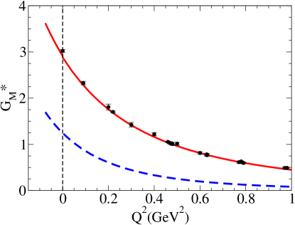
Figure 1: $\gamma^{\ast}N\to\Delta(1232)$ magnetic form factor in the timelike and spacelike region given by the model of Ref. LatticeD . The data for $Q^{2}>0$ is the same as the one presented in Ref. LatticeD . The data for $Q^{2}=0$ is from Ref. Tiator01 . The dashed line represents the contributions of the valence quark core (bare contribution). The solid line is the result of the sum of valence quarks and pion cloud contributions.

III.3.2 $\chi$PT motivated model (model 2)

Instead of Eq. (16) for the pion cloud effect we can use a different parametrization, based in a different combination of multipole functions. For instance, in the two-component model from Refs. Frohlich10 ; Wan06 the contribution from the pion cloud is proportional to the function $F_{\rho}$, interpreted as the $\rho-$propagator, derived from $\chi$PT. This function $F_{\rho}$ was presented in Refs. Iachello73 ; Wan06 ; Iachello04 taking into account the pion loop contributions to the $\rho-$propagator. Here we simplified the exact expression in those references by assuming its limit when $q^{2}\gg 4m_{\pi}^{2}$, and using the normalization $F_{\rho}(0)=1$. For $Q^{2}=-q^{2}>0$ we obtained then

$$F_{\rho}(q^{2})\simeq\frac{m_{\rho}^{2}}{m_{\rho}^{2}+Q^{2}+{\textstyle\frac{1}{\pi}}\frac{\Gamma_{\rho}^{0}}{m_{\pi}}Q^{2}\log\frac{Q^{2}}{m_{\pi}^{2}}}.$$ (26)

In the previous equation, the physical $\rho$-width $\Gamma_{\rho}^{0}$ was taken to be $\Gamma_{\rho}^{0}=0.149$ GeV. Reference Frohlich10 , uses instead $\Gamma_{\rho}^{0}=0.112$ GeV.

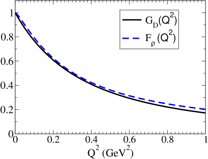
Figure 2: Comparing the dipole form factor $G_{D}$ with the function $F_{\rho}(Q^{2})$ given by Eq. (26).

         

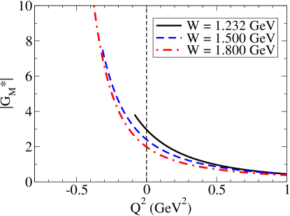
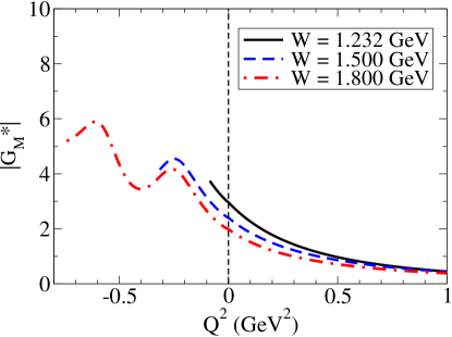
Figure 3: Results for the modulus of the $\gamma N\to\Delta$ magnetic form factor for different $\Delta$ masses ($W$). At left: model 1; at right: model 2. In both cases the valence quark model is from Ref. LatticeD .

Equation (26), derived in the low $q^{2}$ chiral perturbation regime, has a faster falloff for the $\rho$-propagator [with $1/(Q^{2}\log\frac{Q^{2}}{m_{\pi}^{2}})$] than model 1 [with $1/Q^{2}$] for large $Q^{2}$. We used it here to explore alternative parametrizations to model 1 for the pion cloud contributions. The parametrization for the pion cloud contribution (16) is proportional to the dipole factor $\left(\frac{\Lambda_{\pi}^{2}}{\Lambda_{\pi}^{2}+Q^{2}}\right)^{2}$, where $\Lambda_{\pi}$ is a large cutoff, and also to $G_{D}$, the dipole form factor. Although the dipole factor depending on $\Lambda_{\pi}$ was chosen phenomenologically and determined by a fit to the data, one has no reason a priori to use the particular form of $G_{D}$ to parameterize an extra falloff of $G_{M}^{\pi}$. The inclusion of $G_{D}$ was motivated by the traditional convention of dividing the form factor $G_{M}^{\ast}$ by $3G_{D}$ when showing results. With the parametrization (16) one has an asymptotic dependence of $G_{M}^{\pi}\propto 1/Q^{8}$.

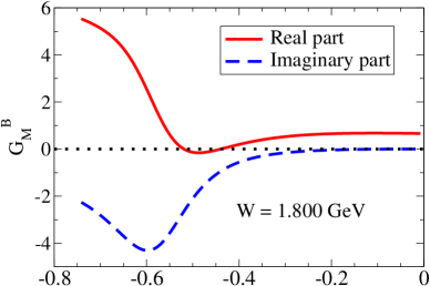
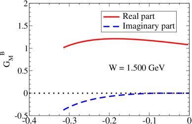
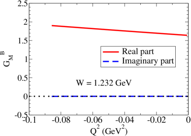
Figure 4: Valence contribution for $\gamma N\to\Delta(1232)$ magnetic form factor for $W=1.232,1.500$ and 1.800 GeV.

We note that in the spacelike region where the pion cloud effects are more important, $0<Q^{2}<1$ GeV², the functions $G_{D}$ and $F_{\rho}$ give very similar results, as seen in Fig. 2. This suggests that one can also use

$$G_{M}^{\pi}(Q^{2})=3\lambda_{\pi}F_{\rho}(q^{2})\left(\frac{\Lambda_{\pi}^{2}}{\Lambda_{\pi}^{2}-q^{2}}\right)^{2},$$ (27)

with

$$F_{\rho}(q^{2})=\frac{m_{\rho}^{2}}{m_{\rho}^{2}-q^{2}-{\textstyle\frac{1}{\pi}}\frac{\Gamma_{\rho}^{0}}{m_{\pi}}q^{2}\log\frac{q^{2}}{m_{\pi}^{2}}+i\frac{\Gamma_{\rho}^{0}}{m_{\pi}}q^{2}},$$ (28)

to extend Eq. (26) to the timelike kinematics. The imaginary part in Eq. (28) is a consequence of two pion production (or transition $\rho\to 2\pi$) which is possible in the timelike region when $q^{2}\geq 4m_{\pi}^{2}$.

We will call the model defined by Eq. (27) model 2. One implication of the new form for the pion cloud contributions is a falloff as $1/(q^{6}\log q^{2})$, slower than for model 1 [$1/q^{8}$ falloff]. [Note that $G_{D}\propto 1/q^{4}$ and $F_{\rho}\propto 1/(q^{2}\log q^{2})$]

Another important feature of the function (27) is that its imaginary part does not peak for $q^{2}=m_{\rho}^{2}\simeq 0.6$ GeV² but for $q^{2}\simeq 0.3$ GeV², because of the logarithm corrections. That effect changes the $Q^{2}$ dependence of the pion cloud contributions to $G_{M}^{\ast}$, relatively to model 1.

A note about $F_{\rho}(q^{2})$ given by Eq. (28): it was derived from the exact result in Refs. Frohlich10 ; Iachello73 ; Iachello04 in the limit $q^{2}\gg 4m_{\pi}^{2}\simeq 0.08$ GeV², as explained before. However, we have checked that our simplified formula, although approximate, does not deviate too much from the exact one, even when that limit does not hold. Therefore our formula gives a good qualitative description of the chiral behavior in the whole domain $q^{2}>0$. We note only that the results from Eq. (28) and the results in Refs. Frohlich10 ; Iachello73 ; Iachello04 differ in a slight deviation of the location of the peak of the imaginary part of $F_{\rho}$. Using Eq. (28) the peak is at $q^{2}\simeq 0.3$ GeV², while in Ref. Frohlich10 ; Iachello73 ; Iachello04 the peak is at $q^{2}\simeq 0.4$ GeV².

Finally, as for the quark current (17) in the bare quark contributions, we will not replace our parametrization of the $\rho$-propagator (18) by (26) since they differ substantially and our parametrization was already calibrated by the physical data Nucleon ; NDelta ; NDeltaD and lattice data Lattice ; LatticeD for the nucleon and $\Delta(1232)$ systems, in the spacelike region. A different parametrization for timelike and spacelike regions would be inconsistent.

IV Results

We will divide the presentation of our results into two parts. In the first part we show the results of the magnetic form factor $G_{M}^{\ast}$, calculated with the two models described in the previous section. In the second part we show the results for the width functions $\Gamma_{\gamma N}(W)$ and $\Gamma_{e^{+}e^{-}N}(W)$, and also for the $\Delta$ mass distribution function $g_{\Delta}(W)$.

IV.1 Form factors in the timelike region

Contrarily to what happens in the spacelike domain, in the timelike region the form factor $G_{M}^{\ast}$ has a non-zero imaginary part. Because of Eq. (7) we are interested in the absolute value of the form factor, $|G_{M}^{\ast}|$, which enters into $|G_{T}(q^{2};W)|^{2}$. Although the form factors are defined for any value of $W\geq M$, we show here results for selected values of $W$ only. We recall that the range of $Q^{2}$ for the function $G_{M}^{\ast}(Q^{2};W)$ depends on $W$, as established by the condition $Q^{2}\geq-(W-M)^{2}$.

The results for $|G_{M}^{\ast}|$ at energies $W=1.232,1.500$ and 1.800 GeV, for both models, are presented in Fig. 3. One notes that the value of $|G_{M}^{\ast}|$ near $Q^{2}=0$ decreases with $W$. We will see that this is a consequence of the valence quark contribution given by Eq. (13). The same effect was observed in lattice QCD simulations where large pion masses induce large nucleon and $\Delta$ masses LatticeD ; Alexandrou08 . In the figure it is also clear that the two models differ substantially in the $Q^{2}$ dependence of $|G_{M}^{\ast}|$. For model 1, $|G_{M}^{\ast}|$ increases as $Q^{2}$ decreases, for all values of $W$, and this behavior is enhanced as $W$ becomes larger. A peak (not shown in the graph because it is too large) is present, near $q^{2}=\Lambda_{D}^{2}\simeq 0.71$ GeV² when $W=1.800$ GeV. A first conclusion is therefore that model 1 generates very strong, and probably unphysical contributions to $|G_{M}^{\ast}|$ in the timelike region. Model 2, in contrast, gives moderated contributions only (larger than in the spacelike region but with the same magnitude) and is therefore a much more reasonable model. To better compare the two models we have to analyze the real and imaginary parts of $G_{M}^{\ast}$ separately.

Since the valence quark contributions are common to both models, we start by looking to the bare term $G_{M}^{B}$. The results are presented in Fig. 4. For $Q^{2}\approx 0$ and values of $W$ not too large when compared with $W=1.232$ GeV, the real part dominates, as expected from the results for the physical case ($W=M_{\Delta}$). For larger values of $W$ and low $Q^{2}$ the real part dominates increasingly less. As for the imaginary part, we recall that is zero down to $Q^{2}\simeq-0.08$ GeV² (because $\Gamma_{\rho}=0$). But as $Q^{2}$ decreases, for larger $W$ values, we can observe the effect of the $\rho$-mass poles emerging at $Q^{2}=-m_{\rho}^{2}\simeq-0.6$ GeV², and strengthening the imaginary parts of $G_{M}^{B}$. For $W=1.800$ GeV the real part also increases in the region $Q^{2}<-m_{\rho}^{2}$ due to the impact of the $\rho$-mass poles. In this case, however, the other terms from the VMD parametrization (17), the constant term and the $M_{h}$-mass poles, are relevant as well. All these contributions to $G_{M}^{B}$ are balanced, and therefore reduced, in the final result, by the pion contributions $G_{M}^{\pi}$ to be discussed next.

We turn now to the term $G_{M}^{\pi}$ which gives the pion cloud contribution, and where the two models differ in the timelike region. The results are presented in Fig. 5 for the same values of $W$ as before. Comparing the two models, we can say that both have similar results for the real part of $G_{M}^{\pi}$ in the region $-0.2$ GeV${}^{2}<Q^{2}$, but differ significantly for smaller values of $Q^{2}$ (larger values of $q^{2}$). That is the consequence of the double pole $q^{2}=\Lambda_{D}^{2}$ in the pion cloud formula for model 1. In model 2 there is no such contribution from the pion cloud and the values for real and imaginary parts are more moderate. Note that the strong peak for $W=1.800$ GeV at $Q^{2}\simeq-0.65$ GeV², for model 1 is a consequence of Eq. (III.3.1), and differs from model 2 by an order of magnitude.

We look now to the imaginary part of $G_{M}^{\pi}$. Our first observation goes to the imaginary part of $G_{M}^{\pi}$ in the region near $Q^{2}=0$. In model 1 it is identically zero for $-0.076\leq Q^{2}\leq 0$ [because $\Gamma_{\rho}=0$ from Eq. (19)], but in model 2 it is different from zero, although small, (this is a consequence of the approximation considered in function $F_{\rho}$ discussed previously). The second observation is that the significant difference between models 1 and 2 is the sign of the imaginary part of $G_{M}^{\pi}$: model 1 gives positive contributions, while model 2 gives negative contributions. This model is motivated by $\chi$PT, satisfies chiral constraints for the $\rho$ propagator, which has a non-analytical pole near $Q^{2}\simeq-0.3$ GeV² present in $F_{\rho}$ and with its origin in the pion loop contributions.

With this detailed analysis we come to understand the large difference between the two models shown in Fig. 3. The figure provides a strong indication that model 1 is not a reasonable model: the results from this model are strongly dominated by the pole $q^{2}=\Lambda_{D}^{2}=0.71$ GeV² which induce extremely large (and probably unphysical) contributions for increasingly large $W$ values. On the other hand, model 2 contains the input from $\chi$PT, and has therefore a more solid basis. The results are very sensitive to this input and clearly exclude model 1.

From the previous discussion we favor the results from model 2. The final results (bare quark core plus pion cloud) for both the real and imaginary part of the form factor $G_{M}^{\ast}$ are presented in Fig. 6. One realizes that the real part dominates over the imaginary part for $Q^{2}>-0.15$ GeV². We can say that the dominant contributions to the imaginary part are the poles from $G_{M}^{\pi}$ (induced by $F_{\rho}$) around $Q^{2}=-0.3$ GeV², and the $\rho$-terms in the quark current from the bare contribution. The effect of those poles is particularly evident in the curve for $W=1.800$ GeV.

       

       

       

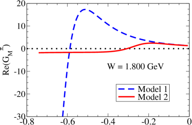
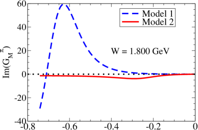
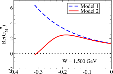
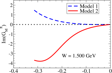
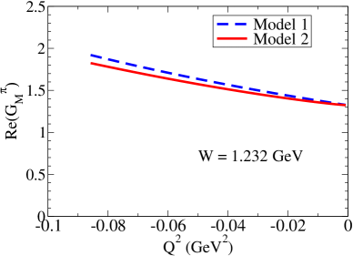
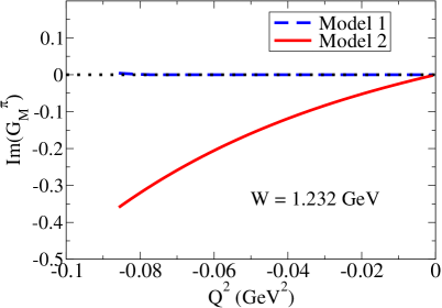
Figure 5: Pion cloud contributions ($G_{M}^{\pi}$) for the $G_{M}^{\ast}$ form factor (real and imaginary parts). The results from models 1 and 2 are shown.

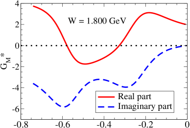
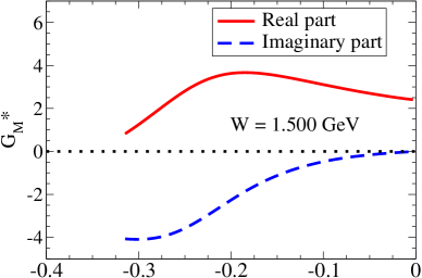
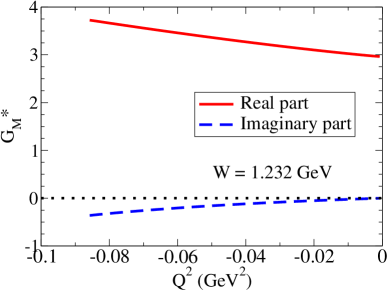
Figure 6: Real and imaginary components of the form factor $G_{M}^{\ast}$ for model 2.

The main and general conclusion from Figs. 4, 5 and 6 is that the final structure for $G_{M}^{\ast}$ emerges from a combination of effects, namely from the VMD model poles and also the pion cloud effects. The two processes interfere crucially and determine the structure of the final amplitude.

Later, we will discuss the applicability of the model for $W>1.8$ GeV, the effect of the remaining poles, and the impact in the observables in consideration. We emphasize that any extension of the $\Delta$ form factors to the timelike region has to rely on models and cannot be directly estimated from experimental data only. It is then important to compare our model with models with a similar content, such as the two-component quark model of Ref. Frohlich10 , also defined in the timelike region. In this last model the contribution from the coupling to the quark core (valence contribution) is 0.3% near $Q^{2}=0$ (99.7% of pion cloud), while in our model one has 55.9% (44.1% of pion cloud). This significant difference between the contributions of the quark core is due to a different, and somewhat arbitrary, classification of the two effects. In the model of Ref. Frohlich10 ; Iachello04 the term from the pion cloud is also classified as an effective part of the VMD mechanism, since it is proportional to the function $F_{\rho}$ for the $\rho$ propagator. Therefore, in that model the VMD mechanism/pion cloud term is the only relevant effect Frohlich10 ; Iachello04 . In our formalism, the coupling with the quarks is calibrated directly by a VMD parametrization and although it gives the dominant contribution, it is not the only one to affect the results. Our model has the advantage of having been tested successfully by the lattice QCD simulations (in a regime where the pion cloud is small), and of agreeing with the EBAC data analysis for the bare quark core contributions to the pion photoproduction data LatticeD . These tests suggest that our estimation of the quark core structure is under control, since the model is largely constrained in a variety of kinematic domains. Another important point is that our model allows a direct physical interpretation of the parameters involved, in terms of the range of the baryon wave functions.

IV.2 Results for $\Gamma_{\gamma N}(W)$ and $\Gamma_{e^{+}e^{-}N}(W)$

We will discuss now the partial widths $\Gamma_{\gamma N}(W)$ and $\Gamma_{e^{+}e^{-}N}(W)$. We will also show $\Gamma_{\pi N}(W)$, given by Eq. (3), together with the calculation of $g_{\Delta}(W)$, defined by Eq. (1).

We start by showing in Fig. 7 the function $\frac{d\Gamma_{e^{+}e^{-}N}}{dq}(W;q)$ for the cases $W=1.232,1.500$ and 1.800 GeV. This figure includes the results from model 1 (dashed line), model 2 (solid line) and also the result of a calculation where the form factor $G_{M}^{\ast}$ is taken as constant, defined by the value of $G_{M}^{\ast}(W,0)$ at the pole $W=M_{\Delta}$ (dotted line), given by the experimental value [$G_{M}^{\ast}(Q^{2})\equiv G_{M}^{\ast}(M_{\Delta},0)\simeq 3.0$]. This last case was also considered in Ref. Frohlich10 and it is useful as a reference for the $q^{2}$ dependence of our results. The figure illustrates that, in line with the results in the previous subsection, for model 1 $\Gamma_{e^{+}e^{-}N}^{\prime}(q,W)$ is enhanced for large $q$ and large $W$ values (see result for $W=1.800$ GeV).

To determine the di-lepton production width, $\Gamma_{e^{+}e^{-}N}(W)$, one has to integrate Eq. (11) using Eq. (10). This is equivalent to calculate the integral of the functions represented in Fig. 7 for each value of $W$ in the interval $[2m_{e},W-M]$. Therefore $\Gamma_{e^{+}e^{-}N}(W)=0$ when $W<M+2m_{e}$. The calculation of the function $\Gamma_{\gamma N}(W)$ proceeds through Eq. (8). The results obtained for the two widths within the three models discussed before, are in Fig. 8.

Finally, $\Gamma_{\pi N}(W)$ is estimated using Eq. (3) and the function

$$q_{\pi}(W)=\frac{\sqrt{\left[(W+M)^{2}-m_{\pi}^{2}\right]\left[(W-M)^{2}-m_{\pi}^{2}\right]}}{2W},$$ (29)

defined for $W\geq M+m_{\pi}$ and $q_{\pi}(W)=0$ otherwise. $\Gamma_{\pi N}(W)$ is then a positive function for $W>M+m_{\pi}$. In Fig. 9 we present the three partial widths obtained with model 2, the one that we favor for the reasons explained in the previous subsection.

We turn now to the $\Delta$ mass distribution function $g_{\Delta}(W)$ defined by Eq. (1). As the channel $\Delta\to\pi N$ is largely dominant, $\Gamma_{tot}(W)\simeq\Gamma_{\pi N}(W)$ and the normalization of $g_{\Delta}(W)$ can be done in that approximation. Considering $\Gamma_{\pi N}(M_{\Delta})\simeq\Gamma_{tot}(M_{\Delta})\simeq\Gamma_{\Delta}^{exp}$, with the experimental result $\Gamma_{\Delta}^{exp}\simeq 0.118$ GeV PDG , one has $A=0.7199$.

The results for the partial contributions to $g_{\Delta}(W)$ are given by

$$g_{\Delta\to\gamma N}(W)=\frac{\Gamma_{\gamma N}(W)}{\Gamma_{tot}(W)}g_{\Delta}(W)$$

$$g_{\Delta\to e^{+}e^{-}N}(W)=\frac{\Gamma_{e^{+}e^{-}N}(W)}{\Gamma_{tot}(W)}g_{\Delta}(W),$$ (30)

and are shown in Fig. 10 for the constant form factor model (dotted line), model 1 (dashed line) and model 2 (solid line). The total results for $g_{\Delta}(W)$ are shown in Fig. 11, for the model 2.

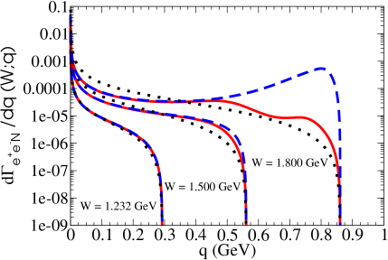
Figure 7: The distribution $\frac{d\Gamma_{e^{+}e^{-}N}}{dq}(W;q)$ as defined in Eqs. (9) and (11) for 3 different energies $W$. The solid line is the result of model 2; the dashed line is the result of model 1 (naive model). The dotted line is the result obtained by using a constant form factor. The function has no dimensions.

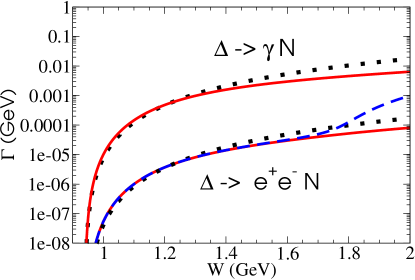
Figure 8: Partial widths as function of $W$ for different models. The constant form factor model is represented by the doted line; the model 1 by the dashed line and the model 2 by the solid line. Note that models 1 and 2 have the same result for the real decay $\Delta\to\gamma N$, because the models are identical at $Q^{2}=0$.

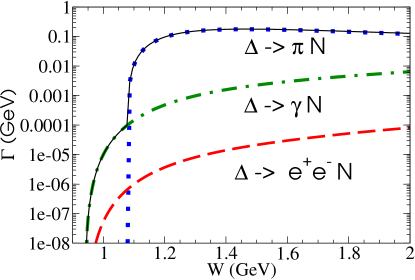
Figure 9: Partial widths as function of $W$ for model 2. The total is represented by the thin solid line.

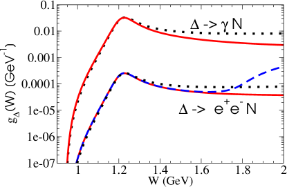
Figure 10: Partial contributions of the channels $\Delta\to\gamma N$ and $\Delta\to e^{+}e^{-}N$ (in GeV^-1 units). The constant form factor model is represented by the doted line; the model 1 by the dashed line and the model 2 by the solid line. Note that models 1 and 2 have the same result for the real decay $\Delta\to\gamma N$, because the models are identical at $Q^{2}=0$.

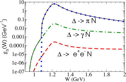
Figure 11: Function $g_{\Delta}(W)$ (in GeV^-1 units) and the partial contributions of the channels $\Delta\to\gamma N,\Delta\to e^{+}e^{-}N$ as function of $W$ for the model 2. The thin solid line is the total result ($g_{\Delta}(W)$) and the sum off all decay channels ($\Delta\to\pi N,\Delta\to\gamma N$ and $\Delta\to e^{+}e^{-}N$).

We restricted our results to the region $W\leq 2$ GeV. Above that region one has to take into account the additional pole structure of the form factor $G_{M}^{\ast}$ that appears for large $q^{2}$ values. Another reason for not having our model applied to larger $W$ values is that, for $W>1.5$ GeV, the reactions are expected to be dominated by resonances as the $N^{\ast}(1440)$, $N^{\ast}(1535)$, $\Delta(1600)$ among others, instead of the $\Delta(1232)$ alone.

As for the first problem, one has to find a way deal with those large $q^{2}$ singularities. From Eq. (27) for the pion cloud component, already, the pole at $q^{2}=\Lambda_{\pi}^{2}\simeq 1.53$ GeV², makes the form factor diverge for $W>M+\Lambda_{\pi}\simeq 2.17$ GeV, since $q^{2}\leq(W-M)^{2}$. Also, from the valence quark component one has a singularity $q^{2}=M_{h}^{2}\simeq 3.53$ GeV². To remove those singularities we may introduce an effective width $\Gamma_{X}$, in analogy with Eq. (18) or (III.3.1), for single or double poles, with a constant width $\Gamma_{X}^{0}$. This procedure adds a new parameter to the model. We started by verifying that a large width $\Gamma_{X}^{0}$ (for instance $\Gamma_{X}^{0}\simeq 1$ GeV) will affect the results for $W<2$ GeV, while a very small width will induce significant oscillations in the functions $g_{\Delta\to\gamma N}(W)$ and $g_{\Delta\to e^{+}e^{-}N}(W)$ (enhancement of $\Gamma^{\prime}_{e^{+}e^{-}N}(q,W)$ near the poles). By taking $\Gamma_{X}^{0}=2\Gamma_{\rho}^{0}$ the results obtained for $W<2$ GeV are almost unchanged, and the results for $W>2$ GeV are also smooth functions of $W$. With this choice the smooth dependence on $W$ of the functions $g_{\Delta\to\gamma N}(W)$ and $g_{\Delta\to e^{+}e^{-}N}(W)$, obtained with model 2 is maintained for higher $W$ values. We stress, nevertheless, that the application of our model to large $W$ values is to be viewed only as an extreme test to its limits.

V Conclusions

In this work we have presented a covariant approach to describe the the Dalitz decays $\Delta\to\gamma N$, $\Delta\to\gamma^{\ast}N$, and we have calculated the $\Delta$ mass distribution function $g_{\Delta}(W)$ within that approach. Our framework can be used to simulate the $NN\to e^{+}e^{-}NN$ reaction at moderate beam kinetic energies ($1-2$ GeV). The code used in this work can be supplied under request.

Our calculations are based on an unified description of the $\gamma^{\ast}N\to\Delta$ reaction, in both the spacelike and timelike regimes. We start with a model tested previously in spacelike physical and lattice QCD simulation data LatticeD ; NDeltaD , and generalize it to the timelike regime. In this formalism the electromagnetic interaction can be decomposed into two mechanisms: the direct photon coupling with the quarks and the interaction with the pion cloud.

For the first mechanism we extended the quark current and wave functions, obtained for $q^{2}<0$, to the region $q^{2}>0$ without additional changes, except for a non-zero width of the effective vector mesons included in the VMD parametrization of our quark electromagnetic current. For the pion cloud contribution we probed two different parametrizations: a naive generalization of our spacelike model and a more elaborated model based on $\chi$PT. Although the two models behave very similarly in the spacelike region, they differ substantially in the timelike region.

The results of the models for the form factor $G_{M}^{\ast}$, as a function of $q$ and $W$, are used to calculate the partial widths $\Gamma_{\gamma N}(W)$, $\Gamma_{\Delta\to e^{+}e^{-}N}(W)$ and the partial mass distributions functions $g_{\Delta\to\gamma N}(W)$, $g_{\Delta\to e^{+}e^{-}N}(W)$.

A first important conclusion of this work is that the $q^{2}$ dependence of the form factor has an impact in the final results, and has therefore to be under control: the results for the $\Delta$ mass distribution functions, where the form factor is taken with its full $q^{2}$ dependence, can differ by a factor of 4 from the results obtained with the constant form factor model.

We verified also that the results are sensitive to the analytical extension of the pion cloud parametrization to the timelike region. Model 1 (naive model) generates unreasonably large contributions for moderate squared momentum $q^{2}$, for larger values of $W$, as consequence of a spurious (not physically motivated) pole $q^{2}=\Lambda_{D}^{2}$ in the pion cloud contribution. Model 2 is motivated by $\chi$PT and includes the function $F_{\rho}$ for the $\rho$ propagator with a non-algebraic pole near $q^{2}\simeq 0.3$ GeV² originated by pion loop corrections. This model gives smooth contributions to the partial $\Delta$ mass distribution functions $g_{\Delta\to\gamma N}(W)$ and $g_{\Delta\to e^{+}e^{-}N}(W)$ that vary slowly with $W$ for large $W$.

A second important conclusion is then that our calculations support the need to have under control the effect of the pion cloud contributions. Our framework is suitable for this because its bare quark core component is constrained by experimental data and lattice QCD simulation data. In addition, the fact that the pion cloud content of model 2 is consistent with $\chi$PT makes model 2 reliable, at least in its domain of validity. The results of model 2 give moderated contributions for $|G_{M}^{\ast}|^{2}$ (since it has no spurious pole at $q^{2}=\Lambda_{D}^{2}$), which are determined by the combined effect of two important features: the pion cloud term structure near $q^{2}=0.3$ GeV², and the quark core contributions from the $\rho-$pole included in the VMD structure of the quark current, near $q^{2}=0.6$ GeV².

We may say that while spacelike data does not constrain models sufficiently well enough, timelike data for ${\textstyle\frac{d\Gamma_{e^{+}e^{-}N}}{dq}}$ for different values of $W$ (see Fig. 7) are important and necessary to select between models in a decisive way. In the $\Delta$ case discussed in this work this is specially true for the pion cloud effects. But the timelike data can also be useful to calibrate the widths and high mass poles of the VMD parametrization of the current needed in valence quark component, particularly for resonances heavier that the $\Delta(1232)$.

For high values of $W$ the assumption that the $\Delta(1232)$ resonance is the only state playing a role in the reactions becomes questionable. In the regime $W>1.5$ GeV other resonances can be relevant, as the spin 1/2 resonances $N^{\ast}(1440)$ and $N^{\ast}(1535)$. Once those states are calibrated for the $Q^{2}=0-2$ GeV² region, one can extend the models from Refs. Roper ; S11 to the timelike region too. It is also expected that the spin 3/2 channels as the $\Delta(1600)$ state are important for large $W$. This defines a study of high interest, since the constraints in the spacelike region are very scarce, and the available data at the photon point suggest a strong contribution from the pion cloud Delta1600 .

Future applications of our formalism can include the study of the $\gamma^{\ast}N\to N$ reaction where the final nucleon has an arbitrary mass $W$, also in the timelike region. Since the quark current was already defined in the timelike region and we have already a model for the nucleon system Nucleon , no additional ingredients are necessary. Such study may provide an important theoretical input to the study of the reaction $p\bar{p}\to\pi^{0}e^{+}e^{-}$ in complement to the first investigation presented here.

Acknowledgments:

The authors want to thank Beatrice Ramstein the comments and the careful reading of the manuscript. The authors thank Catarina Quintans and Piotr Salabura for helpful discussions. G. R. was supported by the Fundação para a Ciência e a Tecnologia under the Grant No. SFRH/BPD/26886/2006. This work is also supported partially by the European Union (HadronPhysics2 project “Study of Strongly Interacting Matter”) and by the Fundação para a Ciência e a Tecnologia, under Grant No. PTDC/FIS/113940/2009, “Hadron Structure with Relativistic Models”.

Appendix A Kinematics

We consider here the final state of the decay process of a resonance $R$ according to $R\to\gamma^{\ast}N$. Assuming $W$ as the invariant mass of the resonance, we can write the four-momentum in the rest frame of $R$ as $P_{R}=(W,{\bf 0})$. In this frame we can also write

$$P_{N}=(E_{N},-{\bf q}),\hskip 28.45274ptq=(\omega,{\bf q}),$$ (31)

where $q$ is the photon momentum: $P_{R}=P_{N}+q$, with $E_{N}=\sqrt{M^{2}+{\bf q}^{2}}$ ($M$ is the nucleon mass). We define then ${\bf q}$ as the photon three momentum (symmetric to the nucleon three momentum) in the final state, and $\omega$ as the photon energy in the $R$ rest frame. All those variables are related with $W^{2}$ and $q^{2}$ according to

$${\bf q}^{2}=\frac{(W^{2}+M^{2}-q^{2})^{2}}{4W^{2}}-M^{2}$$ (32)

$$\omega\equiv\frac{P_{R}\cdot q}{W}=\frac{W^{2}-M^{2}+q^{2}}{2W}.$$ (33)

In the last relation we used $E_{N}={\textstyle\frac{W^{2}+M^{2}-q^{2}}{2W}}$. From Eq. (32) we can conclude that ${\bf q}^{2}$ decreases when $q^{2}$ increases. As ${\bf q}^{2}\geq 0$, it can be proved that there is an upper limit to $q^{2}$ (given by the condition ${\bf q^{2}}=0$). The upper limit is then

$$\left.q^{2}\right|_{\rm max}=(W-M)^{2}.$$ (34)

This is then the largest value of $q^{2}$ for which the timelike form factors are defined.

In conclusion, the timelike form factors are defined only in a limited interval $[0,(W-M)^{2}]$. One has then different ranges according to the value of $W$. In the case $W=M$ we have only $q^{2}=0$. At the pole $W=1.232$ GeV the maximum value of $q^{2}$ is 0.0859 GeV². For $W=1.500$ GeV and $W=1.800$ GeV the maximum value of $q^{2}$ is respectively 0.315 GeV² and 0.741 GeV².

References

- (1) V. D. Burkert and T. S. H. Lee, Int. J. Mod. Phys. E 13, 1035 (2004) [arXiv:nucl-ex/0407020].
- (2) I. G. Aznauryan and V. D. Burkert, Prog. Part. Nucl. Phys. 67, 1 (2012) [arXiv:1109.1720 [hep-ph]].
- (3) I. G. Aznauryan et al. [CLAS Collaboration], Phys. Rev. C 80, 055203 (2009) [arXiv:0909.2349 [nucl-ex]].
- (4) F. Gross, Phys. Rev. 186, 1448 (1969); F. Gross, J. W. Van Orden and K. Holinde, Phys. Rev. C 45, 2094 (1992).
- (5) F. Gross, G. Ramalho and M. T. Peña, Phys. Rev. C 77, 015202 (2008) [arXiv:nucl-th/0606029].
- (6) G. Ramalho, M. T. Peña and F. Gross, Eur. Phys. J. A 36, 329 (2008) [arXiv:0803.3034 [hep-ph]].
- (7) G. Ramalho, M. T. Peña and F. Gross, Phys. Rev. D 78, 114017 (2008) [arXiv:0810.4126 [hep-ph]].
- (8) G. Ramalho, K. Tsushima and F. Gross, Phys. Rev. D 80, 033004 (2009) [arXiv:0907.1060 [hep-ph]].
- (9) G. Ramalho, F. Gross, M. T. Peña and K. Tsushima, Proceedings of Excusive Reactions and High Momentum Transfer IV, 287 (2011) [arXiv:1008.0371 [hep-ph]].
- (10) F. Gross, G. Ramalho and M. T. Peña, arXiv:1201.6336 [hep-ph], to appear in Phys. Rev. D.
- (11) F. Gross, G. Ramalho and M. T. Peña, arXiv:1201.6337 [hep-ph], to appear in Phys. Rev. D.
- (12) G. Ramalho and M. T. Peña, Phys. Rev. D 80, 013008 (2009) [arXiv:0901.4310 [hep-ph]].
- (13) G. Ramalho and M. T. Peña, J. Phys. G 36, 115011 (2009) [arXiv:0812.0187 [hep-ph]].
- (14) G. Ramalho and K. Tsushima, Phys. Rev. D 82, 073007 (2010) [arXiv:1008.3822 [hep-ph]].
- (15) G. Ramalho and K. Tsushima, Phys. Rev. D 81, 074020 (2010) [arXiv:1002.3386 [hep-ph]].
- (16) G. Ramalho and M. T. Peña, Phys. Rev. D 84, 033007 (2011) [arXiv:1105.2223 [hep-ph]].
- (17) G. Ramalho and K. Tsushima, Phys. Rev. D 84, 051301 (2011) [arXiv:1105.2484 [hep-ph]].
- (18) G. Ramalho and K. Tsushima, Phys. Rev. D 84, 054014 (2011) [arXiv:1107.1791 [hep-ph]].
- (19) F. Dohrmann et al., Eur. Phys. J. A 45, 401 (2010) [arXiv:0909.5373 [nucl-ex]].
- (20) M. Zetenyi and G. Wolf, Phys. Rev. C 67, 044002 (2003) [arXiv:nucl-th/0103062].
- (21) L. P. Kaptari and B. Kampfer, Nucl. Phys. A 764, 338 (2006) [arXiv:nucl-th/0504072].
- (22) L. P. Kaptari and B. Kampfer, Phys. Rev. C 80, 064003 (2009) [arXiv:0903.2466 [nucl-th]].
- (23) G. Agakishiev et al. [HADES Collaboration], Phys. Lett. B 690, 118 (2010) [arXiv:0910.5875 [nucl-ex]].
- (24) R. Shyam, U. Mosel, Phys. Rev. C82, 062201 (2010) [arXiv:1006.3873 [hep-ph]].
- (25) G. Agakishiev et al. [HADES Collaboration], arXiv:1112.3607 [nucl-ex], to be published in Eur. Phys. J. A.
- (26) J. Weil, H. van Hees and U. Mosel, arXiv:1203.3557 [nucl-th].
- (27) P. Tlusty [HADES Collaboration], AIP Conf. Proc. 1322, 116 (2010).
- (28) G. Agakichiev et al. [HADES Collaboration], Phys. Rev. Lett. 98, 052302 (2007) [arXiv:nucl-ex/0608031]; G. Agakishiev et al. [HADES Collaboration], Phys. Lett. B 663, 43 (2008) [arXiv:0711.4281 [nucl-ex]]; G. Agakishiev et al. [HADES Collaboration], Phys. Rev. C 84, 014902 (2011) [arXiv:1103.0876 [nucl-ex]].
- (29) V. Pascalutsa, M. Vanderhaeghen and S. N. Yang, Phys. Rept. 437, 125 (2007) [arXiv:hep-ph/0609004].
- (30) S. Teis, W. Cassing, M. Effenberger, A. Hombach, U. Mosel and G. Wolf, Z. Phys. A 356, 421 (1997) [arXiv:nucl-th/9609009].
- (31) G. Wolf, G. Batko, W. Cassing, U. Mosel, K. Niita and M. Schaefer, Nucl. Phys. A 517, 615 (1990).
- (32) M. I. Krivoruchenko and A. Faessler, Phys. Rev. D 65, 017502 (2001) [arXiv:nucl-th/0104045].
- (33) H. F. Jones and M. D. Scadron, Annals Phys. 81, 1 (1973).
- (34) Q. Wan and F. Iachello, Int. J. Mod. Phys. A 20, 1846 (2005).
- (35) F. Iachello and Q. Wan, Phys. Rev. C 69, 055204 (2004).
- (36) R. Bijker and F. Iachello, Phys. Rev. C 69, 068201 (2004) [arXiv:nucl-th/0405028].
- (37) Q. Wan, “A unified approach to baryon electromagnetic form factors,” UMI-32-43721, PhD thesis (2006).
- (38) F. Iachello, A. D. Jackson and A. Lande, Phys. Lett. B 43, 191 (1973).
- (39) M. I. Krivoruchenko, B. V. Martemyanov, A. Faessler and C. Fuchs, Annals Phys. 296, 299 (2002) [arXiv:nucl-th/0110066].
- (40) C. Alexandrou, G. Koutsou, H. Neff, J. W. Negele, W. Schroers and A. Tsapalis, Phys. Rev. D 77, 085012 (2008) [arXiv:0710.4621 [hep-lat].
- (41) B. Julia-Diaz, T. S. Lee, T. Sato and L. C. Smith, Phys. Rev. C 75, 015205 (2007) [arXiv:nucl-th/0611033].
- (42) K. Nakamura et al. [Particle Data Group], J. Phys. G 37, 075021 (2010).
- (43) H. B. O’Connell, B. C. Pearce, A. W. Thomas and A. G. Williams, Phys. Lett. B 354, 14 (1995) [arXiv:hep-ph/9503332].
- (44) H. B. O’Connell, B. C. Pearce, A. W. Thomas and A. G. Williams, Prog. Part. Nucl. Phys. 39, 201 (1997) [arXiv:hep-ph/9501251].
- (45) G. J. Gounaris, J. J. Sakurai, Phys. Rev. Lett. 21, 244-247 (1968).
- (46) L. Tiator, D. Drechsel, O. Hanstein, S. S. Kamalov and S. N. Yang, Nucl. Phys. A 689, 205 (2001) [arXiv:nucl-th/0012046].