Detectability of Symbol Manipulation by an Amplify-and-Forward Relay

Abstract

This paper studies the problem of detecting a potential malicious relay node by a source node that relies on the relay to forward information to other nodes. The channel model of two source nodes simultaneously sending symbols to a relay is considered. The relay is contracted to forward the symbols that it receives back to the sources in the amplify-and-forward manner. However there is a chance that the relay may send altered symbols back to the sources. Each source attempts to individually detect such malicious acts of the relay by comparing the empirical distribution of the symbols that it receives from the relay conditioned on its own transmitted symbols with known stochastic characteristics of the channel. It is shown that maliciousness of the relay can be asymptotically detected with sufficient channel observations if and only if the channel satisfies a non-manipulable condition, which can be easily checked. As a result, the non-manipulable condition provides us a clear-cut criterion to determine the detectability of the aforementioned class of symbol manipulation attacks potentially conducted by the relay.

I Introduction

It is a commonplace in many communication networks that no direct physical link exists between the source and destination nodes of an information flow. Thus information needs to be relayed from the source to the destination through intermediate nodes. This requirement brings forth a major security question: How is one able to ensure that the intermediate nodes faithfully forward information from the source to the destination? Trust management [1]–[3] is a widely researched approach to address this question. In essence, trust management pertains to the establishment, distribution, and maintenance of trust relationships among nodes in a network. Based upon such relationships, it is expected that trusted nodes will faithfully operate according to some protocols that they have agreed upon.

The aforementioned trust relationships are primarily quantified using trust metrics that are evaluated through nodes interacting with and observing the behaviors of each other [4]–[9]. For nodes that do not directly interact with each other, trust relationships can be established and maintained via inference [10]. It is clear that the valuation of trust metrics is critically important in this trust management approach. Many different ways have been proposed to evaluate the trust metrics based on authentication keys [11, 12, 13], reputation [14, 15], and evidence collected from network as well as physical interaction [16, 17, 18]. Given the complexity and difficulty involved in quantifying the vague notion of trust, one would expect these valuation schemes are naturally ad hoc.

To more systematically construct a trust metric, one needs to specify the class of malicious actions against which the metric measures. In this paper, we consider a class of data manipulation attacks in which intermediate nodes may alter the channel symbols that they are supposed to forward. We cast the trust metric valuation problem as a maliciousness detection problem against this class of attacks. More precisely, a node (or another trusted node called a watchdog [19]) detects if another node relays manipulated symbols that are different from those originally sent out by the node itself. Observations for detection against the malicious attack can be made in the physical and/or higher layers.

Most existing maliciousness detection methods are key-based, requiring at the minimum the source and destination nodes to share a secret key that is not privy to the relay node being examined. In [20], keys, which correspond to vectors in a null space, are given to all nodes in a network. Any modification to the encrypted data by a relay node can be checked by determining whether the observed data falls into the null space or not. In [21], symmetric cryptographic keys are applied to the data at source and destination for the purpose of checking the maliciousness of relay node(s). Another key-based approach is considered in [22] by measuring whether only a small amount of packets are dropped by relay nodes. In [23], a cross-layer approach based on measurement of channel symbols is taken. Two keys are employed in that scheme; one to create a set of known data and another to make the data indistinguishable from the key. When the destination receives the message, the probability of error of the transmitted values of the key can be used to determine if the relay node is acting maliciously. In all, the key-based maliciousness detection schemes described above are far from desirable as they require the support of some key distribution mechanism, which in turn presumes the existence of inherently trusted nodes in the network. Moreover some key-based methods have been shown insecure in [24] when nondeterminism and bit-level representation of the data is considered.

For the class of symbol manipulation attacks, it is intuitive that maliciousness of a node should be detected by the nearby nodes based on measurements obtained at the lower layers, since such measurements are more reliable than those made by faraway nodes and at the higher layers as there are fewer chances for potential adversaries to tamper with the former measurements. Hence we investigate the maliciousness detectability problem from a physical-layer perspective by considering a model in which two sources want to share information through a potentially untrustworthy relay node that is supposed to relay the information in the amplify-and-forward manner. In [25], we provide a preliminary study on the problem under a restrictive case in which the relay may only modify the channel symbols based on some independent and identically distributed (i.i.d) attack model, and the source nodes can perfectly observe the symbols forwarded by the relay. In this paper, we extend the treatment to a general channel model and an effectively general class of symbol manipulation attacks. The details of the channel and attack models are provided in Section III.

In Section II, we qualitatively discuss maliciousness detectability in a simple binary-input addition channel in order to motivate the detectability problem. This example has been presented in [25]. It is repeated here for easy reference. In Section IV, we state our main result, which is a necessary and sufficient condition on the channel that guarantees asymptotic detection of maliciousness individually by both source nodes using empirical distributions of their respective observations. We also provide algorithms to check for the stated condition. The results presented in Section IV make clear that maliciousness detectability under our model is a consequence of the stochastic characteristics of the channel and the sources. It works solely based on observations made by the source nodes about the symbols sent by the relay node together with knowledge about the channel. No presumed shared secret between any set of nodes is required or used. Thus the proposed maliciousness detection approach can be used independent of or in conjunction with the key-based methods described above to provide another level of protection against adversaries

The proofs of the results in Section IV are provided later in Section VI. In Section V, we present results from numerical simulation studies of the addition channel example in Section II and other more complicated channels to illustrate the asymptotic detectability results in Section IV with finite observations. Finally we draw a few conclusions about this work in Section VII.

II Motivating Example

To motivate the maliciousness detectability model and results in later sections, let us first consider the simple binary-input addition channel shown in Fig. 1, in which two source nodes (Alice & Bob) communicate to one another through a relay node (Romeo) in discrete time instants.

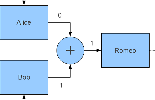
Figure 1: Motivating example of a binary-input addition channel.

The source alphabets of Alice and Bob are both binary $\{0,1\}$. The channel from Alice and Bob to Romeo is defined by the summation of the symbols transmitted by Alice and Bob. Romeo is supposed to broadcast his observed symbol, without modification, back to Alice and Bob. Both Alice and Bob observe the symbol transmitted by Romeo perfectly. Thus the input and output alphabets of Romeo and the observation alphabets of both Alice and Bob are all ternary $\{0,1,2\}$. Alice, for instance, can obtain Bob’s source symbol by subtracting her own source symbol from the symbol transmitted by Romeo.

Now consider the possibility that Romeo may not faithfully forward the symbol that he observes to Alice and Bob in an attempt to impede the communication between them. The main question that we are interested in is whether Alice and Bob are able to discern, from their respective observed symbols, if Romeo is acting maliciously by forwarding symbols that are different than those he has received. To proceed answering this question, let us first consider a single round of transmission, i.e., Alice and Bob transmit their source symbols to Romeo and then Romeo broadcasts a symbol (may be different than what he has received) back to Alice and Bob. Suppose that Alice sends a $0$ and receives a $2$ back from Romeo. Then it will be clear to her that Romeo must have modified what he has received. On the other hand, if Alice receives a $1$ back, then she will not be able to tell whether Romeo has acted maliciously or not. One can continue this line of simple deduction to obtain all the possible outcomes in Table I.

TABLE I: Possible outcomes of the system in Fig. 1.

Alice	Bob	Romeo	Romeo	Detection Outcome
		In	Out
0	0	0	0	Not malicious
			1	Not detected
			2	Alice & Bob both detect
0	1	1	0	Bob detects
			1	Not malicious
			2	Alice detects
1	0	1	0	Alice detects
			1	Not malicious
			2	Bob detects
1	1	2	0	Alice & Bob both detect
			1	Not detected
			2	Not malicious

It is clear from the table that neither Alice nor Bob will be able to determine if Romeo is malicious in general from a single round of transmission.

However the situation changes if Alice and Bob know the source distributions of one another and are allowed to decide on the maliciousness of Romeo over multiple rounds of transmission. To further elaborate, suppose that the source symbols of Bob and Alice are i.i.d. Bernoulli random variables with parameter $\frac{1}{2}$. Then the probabilities of the events that Romeo’s input symbol takes on the values $0$, $1$, and $2$ are $\frac{1}{4}$, $\frac{1}{2}$, and $\frac{1}{4}$, respectively. In particular, out of many rounds of transmission one would expect half of the symbols transmitted by Romeo be $1$’s. From Table I, we see that for Romeo to be malicious and remained undetected by neither Alice nor Bob, he can only change a $0$ to a $1$ and a $2$ to a $1$ in any single round of transmission. But if he does so often, the number of $1$’s that he sends out will be more than half of the number of transmission rounds, as expected from normal operation. On the other hand, Romeo can fool one of Alice and Bob by changing a $1$ to either a $0$ or $2$. But he is not able to determine in each change whether Alice or Bob is fooled. Hence over many such changes the probability of not being detected become decreasingly small. In summary, Alice and Bob may individually deduce any maliciousness of Romeo by observing the distribution of Romeo’s output symbol conditioned on their respective own input symbols. This capability is induced by the restrictions on what Romeo can do that are imposed by the characteristic of the addition channel depicted in Fig. 1. It is important to notice that Alice and Bob do not need to possess any shared secret that is not privy to Romeo.

III System Model

III-A Notation

Let $a$ be a $1\!\times\!m$ row vector and $A$ be a $m\!\times\!n$ matrix. For $i=1,2,\ldots,m$ and $j=1,2,\ldots,n$, $a_{i}$ and $[a]_{i}$ both denote the $i$th element of $a$, and $A_{i,j}$ and $[A]_{i,j}$ both denote the $(i,j)$th element of $A$. Whenever there is no ambiguity, we will employ the unbracketed notation for simplicity. Moreover, we write the $i$th row of $A$ as $A_{i}$. Of course, $[A_{i}]_{j}=A_{i,j}$. Let the transpose of $A$ be denoted by $A^{T}$. Then the $j$th column of $A$ is $(A^{T}_{j})^{T}$. It is our convention that all column vectors are written as the transposes of row vectors. For instance, $a$ is a row vector and $a^{T}$ is a column vector. The $L_{1}$-norm of $a$ is $\|{a}\|_{1}=\sum_{i=1}^{m}|a_{i}|$, while the Euclidean norm of $a$ is $\|{a}\|_{2}=\sqrt{aa^{T}}$. The operation $\mathrm{vec}(A)$ vectorizes the matrix $A$ by stacking its columns to form a $mn\!\times\!1$ column vector. We define $\|{A}\|_{1}\triangleq\|{\mathrm{vec}(A)}\|_{1}$ and $\|{A}\|_{2}\triangleq\|{\mathrm{vec}(A)}\|_{2}$. Note that $\|{A}\|_{2}$ is the Frobenius norm of $A$. The identity and zero matrices of any dimension are denoted by the generic symbols $I$ and $0$, respectively.

Let $X$ be a discrete random variable. We use $|X|$ to denote the size of the alphabet of $X$. Our convention is to use the corresponding lowercase letter to denote the elements in the alphabet of a random variable. For example, the alphabet of $X$ is $\{x_{1},x_{2},\ldots,x_{|X|}\}$. We denote the probability mass function (pmf) $\Pr(X=x_{j})$ by $p(x_{j})$. In addition, let $X$ and $Y$ be two discrete random variables. We denote the conditional pmf $\Pr(Y=y_{i}|X=x_{j})$ by $p(y_{i}|x_{j})$ for simplicity. Let $x^{N}$ denote a sequence of $N$ symbols drawn from the alphabet of $X$. The counting function $\pi(x_{i};x^{N})$ denotes the number of occurrences of $x_{i}$, the $i$th symbol in the alphabet of $X$ as described above, in the sequence $x^{N}$. Let $1_{n}(x_{i};x^{N})$ be the indicator function of the condition that the $n$th symbol in the sequence $x^{N}$ is $x_{i}$. Then we clearly have

$$\pi(x_{i};x^{N})=\sum_{n=1}^{N}1_{n}(x_{i};x^{N}).$$

The counting function also trivially extends to give the number of occurrences of a tuple of symbols drawn from the corresponding tuple of alphabets of random variables. For example, if $x^{N}$ and $y^{N}$ are length-$N$ sequences of symbols drawn from the alphabets of $X$ and $Y$, respectively, then

$$\pi(x_{i},y_{j};x^{N},y^{N})=\sum_{n=1}^{N}1_{n}(x_{i};x^{N})1_{n}(y_{j};y^{N}).$$

The set of typical $X$-sequences (e.g., [26, Definition 6.1]) is denoted by

$$T^{N}_{[X],\delta}\triangleq\left\{x^{N}:\sum_{i=1}^{|X|}\left|\frac{1}{N}\pi(x_{i};x^{N})-p(x_{i})\right|\leq\delta\right\}.$$

Whenever there is no confusion, we write for instance $\pi^{N}(x_{i})$ and $1_{n}^{N}(x_{i})$ in place of $\pi(x_{i};x^{N})$ and $1_{n}(x_{i};x^{N})$, respectively, to simplify notation. Finally, let us define the symbol indexing maps $\chi_{n}(x^{N})$, $n=1,2,\ldots,N$, by assigning the index value $j$ to $\chi_{n}(x^{N})$ when the $n$th symbol in the sequence $x^{N}$ is $x_{j}$, namely, the $j$th element in the alphabet of $X$.

III-B Channel model

Consider the channel model shown in Fig. 2. This model serves as a generalization of the motivating example described in Section I.

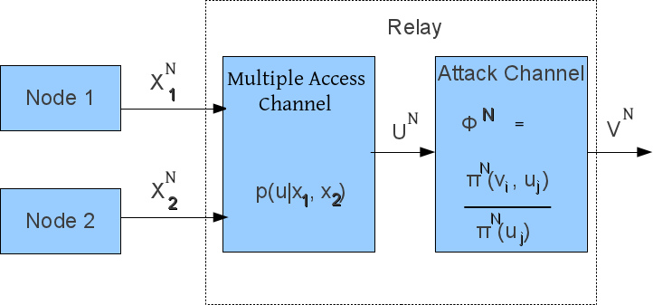
(a) Multiple-access channel (time instants $1,2\ldots,N$)

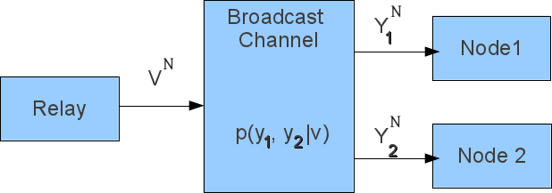
(b) Broadcast channel (time instants $N+1,N+2,\ldots,2N$)

Figure 2: Amplify-and-forward relaying model.

Two nodes (1 and 2) simultaneously forward their source symbols to a relay node. The relay node is supposed to forward its received symbols back to the two nodes (or to some other nodes) in the amplify-and-forward manner. There is some possibility that the relay may modify its received symbols in an attempt to degrade the performance of the transmission. Our goal is to determine if and when it is possible for nodes 1 and 2 to detect any malicious act of the relay by observing the symbols broadcast from the relay in relation to the symbols that they individually transmitted. Note that the above model also covers the perhaps more common scenario in which only one node has information to send while the transmission by the other node is regarded as intentional interference.

More specifically, let $X_{1}$ and $X_{2}$ be two independent discrete random variables that specify the generic distributions of the symbols transmitted by nodes 1 and 2, respectively. At time instants $1,2,\ldots,N$, nodes 1 and 2 transmit i.i.d. symbols respectively distributed according to $X_{1}$ and $X_{2}$. The transmission goes through a memoryless multiple-access channel (MAC) with the random variable $U$ describing its generic output symbol. The MAC is specified by the conditional pmf $p(u_{k}|x_{1,i},x_{2,j})$. The relay node, during time instants $1,2,\ldots,N$, observes the output symbols of the MAC, processes (or manipulates) them, and then broadcasts the processed symbols out to nodes 1 and 2 at time instants $N+1,N+2,\ldots,2N$ via a memoryless broadcast channel (BC) with the random variables $V$ describing its generic input symbol and $Y_{1}$ and $Y_{2}$ describing the generic output symbols at nodes 1 and 2, respectively. The BC is specified by the conditional pmf $p(y_{1,i},y_{2,j}|v_{k})$. In addition, because the relay is supposed to work in the amplify-and-forward manner, we adopt the reasonable model that the alphabets of $U$ and $V$ are of the same size, and there is a one-to-one correspondence $u_{i}\leftrightarrow v_{i}$, $i=1,2,\ldots,|U|$, between elements of the alphabets.

Let $u^{N}$ denote the sequence of $N$ output symbols of the MAC observed by the relay during time instants $1,2,\ldots,N$, and $v^{N}$ denote the sequence of $N$ input symbols of the BC transmitted by the relay during time instants $N+1,N+2,\ldots,2N$. Then the mapping $v^{N}=\phi^{N}(u^{N})$ represents the manipulation performed by the relay. The manipulation map $\phi^{N}$ is allowed to be arbitrary, deterministic or random, and known to neither node 1 nor 2. The only restriction we impose is the Markovity condition that $p(v^{N}|u^{N},x_{1}^{N},x_{2}^{N})=p(v^{N}|u^{N})$, where $x_{1}^{N}$ and $x_{2}^{N}$ denote the symbol sequences transmitted by nodes 1 and 2, respectively, during time instants $1,2,\ldots,N$. That is, the relay may potentially manipulate the transmission based only on the output symbols of the MAC that it observes.

III-C Maliciousness of relay

Consider the $|U|\!\times\!|U|$ matrix $\Phi^{N}$ whose $(i,j)$th element is defined by

$$\Phi^{N}_{i,j}\triangleq\frac{\pi^{N}(v_{i},u_{j})}{\pi^{N}(u_{j})}.$$ (1)

It is obvious that $\Phi^{N}$ is a stochastic matrix describing a valid conditional pmf of a fictitious channel, which we will refer to as the attack channel. Despite omitted from its notation, the attack channel $\Phi^{N}$ depends on the sequences $u^{N}$ and $v^{N}$. Rather than directly acting on the MAC output symbols to produce input symbols for the BC, the attack channel $\Phi^{N}$ extracts the statistical properties of the manipulation map $\phi^{N}$ that are relevant to our purpose of defining (and later detecting) the maliciousness of the action of the relay:

Definition 1.

(Maliciousness) The relay is said to be non-malicious if $\|{\Phi^{N}-I}\|_{1}\rightarrow 0$ in probability as $N$ approaches infinity. Otherwise, the relay is considered malicious.

In the strictest sense, normal amplify-and-forward relay operation should require $\Phi^{N}=I$ for all $u^{N}$ and $v^{N}$ and for each $N$. Nevertheless it turns out to be beneficial to consider the relaxation in Definition 1 when the primary focus is to check whether the relay is degrading the channel rather than attacking a specific part of the transmission. In particular, the probabilistic and limiting relaxation in Definition 1 allows us to obtain definite results (see Section IV) for the very general class of potential manipulation maps described above by tolerating actions, such as manipulating only a negligible fraction of symbols, that have essentially no effect on the information rate across the relay. We point out that it is possible to develop similar results based on the above-mentioned strictest sense of maliciousness for some more restricted classes of manipulation maps (see [25] for instance).

III-D Maliciousness detection

Due to symmetry, it suffices to focus on node 1’s attempt to detect whether the relay is acting maliciously or not. To that end, we are particularly interested in the “marginalized” MAC pmf $p(u_{i}|x_{1,j})$ and marginal BC pmf $p(y_{1,i}|v_{j})$. For better bookkeeping, we will write the two conditional pmfs in terms of the $|U|\!\times\!|X_{1}|$ matrix $A$ and $|Y_{1}|\!\times\!|U|$ matrix $B$ whose elements are respectively defined by

$$A_{i,j} \triangleq p(u_{i}|x_{1,j})$$

$$B_{i,j} \triangleq p(y_{1,i}|v_{j}).$$

To complete the bookkeeping process, we define the $|Y_{1}|\!\times\!|X_{1}|$ matrix $\Gamma^{N}$ as

$$\Gamma^{N}\triangleq B\Phi^{N}A,$$ (2)

which can be interpreted as the conditional pmf of the node 1’s observation if the relay were to act in an i.i.d. manner described by the attack channel $\Phi^{N}$.

We assume that node 1 knows $A$ and $B$. We will refer to the pair $(A,B)$ as the observation channel for node 1, which may use knowledge about the observation channel to detect any maliciousness of the relay. Justifications for this assumption can be made based on applying knowledge of the physical MAC and BC in a game-theoretic argument similar to the one given in [23]. Before data communication between the nodes and relay takes place, they must agree on a relaying protocol. During the negotiation process of such protocol, the relay needs to either reveal $A$ and $B$ to the nodes, or provide assistant to the nodes to learn $A$ and $B$. If the relay provides false information about $A$ and $B$ corresponding to a more favorable channel environment than the actual one, the nodes may use the knowledge of the physical channel to check against the false information. On the other hand, it would also not be beneficial for the relay to misinform the nodes with a less favorable channel environment, since in such case the nodes may simply decide not to use the relay.

We may also assume that $A$ contains no all-zero rows and that $p(x_{1,j})>0$ for all $x_{1,j}$ in the alphabet of $X_{1}$. If these assumptions do not hold, we can reinforce them by removing symbols from the alphabets of $X_{1}$ and $U$ and deleting the corresponding rows and columns from $A$, without affecting the system model. In addition, note that relabeling of elements in the alphabets of $X_{1}$ and $Y_{1}$ amounts to permuting the columns of $A$ and rows of $B$, respectively. Relabelling of elements in the alphabet of $U$, and hence the corresponding elements in the alphabet of $V$, requires simultaneous permutation of the rows of $A$ and columns of $B$. It is obvious that all these relabellings, and hence the corresponding permutations of rows and columns of $A$ and $B$, do not change the underlying system model. Therefore we will implicitly assume any such convenient permutations in the rest of the paper.

As mentioned before, detection of maliciousness of the relay is to be done during normal data transmission. That is, the detection is based upon the symbols that node 1 transmits at time instants $1,2,\ldots,N$ (i.e., $x_{1}^{N}$) and the corresponding symbols that node 1 receives at time instant $N+1,N+2,\ldots,2N$ (i.e., $y_{1}^{N}$). We refer to each pair of such corresponding transmit and receive symbols (e.g., the ones at time instants $1$ and $N+1$) as a single observation made by node 1. Node 1 is free however to use its $N$ observations to detect maliciousness of the relay. For instance, we may employ the following estimator of $\Phi^{N}$ to construct a decision statistic for maliciousness detection. First node 1 obtains the conditional histogram estimator $\hat{\Gamma}^{N}$ of $\Gamma^{N}$ defined by its $(i,j)$th element:

$$\hat{\Gamma}^{N}_{i,j}\triangleq\frac{\pi^{N}(y_{1,i},x_{1,j})}{\pi^{N}(x_{1,j})}.$$ (3)

Then it constructs the estimator $\hat{\Phi}^{N}$ from $\hat{\Gamma}^{N}$ according to:

$$\hat{\Phi}^{N}=\begin{cases}\displaystyle\arg\max_{\hat{\Phi}\in G_{\mu}(\hat{\Gamma}^{N})}\|{\hat{\Phi}-I}\|_{1}&\mbox{if~{}}G_{\mu}(\hat{\Gamma}^{N})\mbox{~{}is non-empty,}\\ I&\mbox{otherwise.}\end{cases}$$ (4)

In (4), $\mu$ is a small positive constant and $G_{\mu}(\hat{\Gamma})$ is the set of $|U|\!\times\!|U|$ stochastic matrices, for each of which (say denoted by $\hat{\Phi}$), there exists a $|Y_{1}|\!\times\!|U|$ stochastic matrix $\tilde{\Gamma}$ such that $\|{\Pi_{B}(\tilde{\Gamma}-\hat{\Gamma})\Pi_{A}}\|_{1}\leq\mu$ and $B\hat{\Phi}A=\Pi_{B}\tilde{\Gamma}\Pi_{A}$, where $\Pi_{A}$ and $\Pi_{B}$ denote the orthogonal projectors onto the row space of $A$ and column space of $B$, respectively. We will employ the estimator $\hat{\Phi}^{N}$ specified in (4) to obtain the detectability results in the following sections.

IV Maliciousness Detectability

To describe the main results of this paper, we first need to introduce the following notions of normalized, balanced, and polarized vectors:

Definition 2.

(Normalized vector) A non-zero vector $\omega$ is said to be normalized if $\|{\omega}\|_{1}=1$.

Definition 3.

(Balanced vector) A vector $\omega$ is said to be balanced if $\sum_{i}\omega_{i}=0$.

Definition 4.

(Polarized vectors) For $b\geq 0$ and $0\leq\epsilon\leq b$, a vector $\omega$ is said to be $(b,\epsilon)$-polarized at $j$ if

$$\omega_{i}\in\begin{cases}[b,\infty)&\mbox{~{}for~{}}i=j\\ (-\infty,\epsilon]&\mbox{~{}for~{}}i\neq j.\end{cases}$$

Further $\omega$ is said to be $(b,\epsilon)$-double polarized at $(j,k)$ if

$$\omega_{i}\in\begin{cases}[b,\infty)&\mbox{~{}for~{}}i=j\\ (-\infty,-b]&\mbox{~{}for~{}}i=k\\ [-\epsilon,\epsilon]&\mbox{~{}for~{}}i\neq j,k.\end{cases}$$

IV-A Main result

The main result of this paper is that detectability of maliciousness of the relay is characterized by the following categorization of observation channels:

Definition 5.

(Manipulable observation channel) The observation channel $(A,B)$ is manipulable if there exists a $|U|\!\times\!|U|$ non-zero matrix $\Upsilon$, whose $j$th column, for each $j=1,2,\ldots,|U|$, is balanced and $(0,0)$-polarized at $j$, with the property that all columns of $\Upsilon A$ are in the right null space of $B$. Otherwise, $(A,B)$ is said to be non-manipulable.

Let $D^{N}=D^{N}(y_{1}^{N},x_{1}^{N})$ denote a decision statistic based on the first $N$ observations $(y_{1}^{N},x_{1}^{N})$ that is employed for maliciousness detection. The following theorem states that maliciousness detectability is equivalent to non-manipulablility of the observation channel:

Theorem 1.

(Maliciousness detectability) When and only when the observation channel $(A,B)$ is non-manipulable, there exists a sequence of decision statistics $\{D^{N}\}$ with the following properties (assuming $\delta>0$ below):

1. If $\limsup_{N\rightarrow\infty}\Pr(\|{\Phi^{N}-I}\|_{1}>\delta)>0$, then

   $$\limsup_{N\rightarrow\infty}\Pr\left(D^{N}>\delta~{}\Big{|}~{}\|{\Phi^{N}-I}\|_{1}>\delta\right)=1.$$

2. If $\liminf_{N\rightarrow\infty}\Pr(\|{\Phi^{N}-I}\|_{1}\leq\delta)>0$, then

   $$\lim_{N\rightarrow\infty}\Pr\left(D^{N}>c\delta~{}\Big{|}~{}\|{\Phi^{N}-I}\|_{1}\leq\delta\right)=0$$

   for some positive constant $c$ that depends only on $A$ and $B$.

The theorem verifies the previous claim that the attack channel $\Phi^{N}$ provides us the required statistical characterization for distinguishing between malicious and non-malicious amplify-and-forward relay. In addition, as shown in the proof of the theorem to be provided later in Section VI-C this distinguishability is (asymptotically) observable through the decision statistic $\|{\hat{\Phi}^{N}-I}\|_{1}$, where $\hat{\Phi}^{N}$ is the estimator of $\Phi^{N}$ described in (4), for non-manipulable channels. The requirement of $(A,B)$ being non-manipulable is not over-restrictive and is satisfied in many practical scenarios.

Theorem 1 can further be employed to characterize detectability of maliciousness of the relay in the context of Definition 1:

Corollary 1.

Given that $(A,B)$ is non-manipulable, the sequence of decision statistics $\{D^{N}\}$ in Theorem 1 also satisfies the following properties:

1. If the relay is not malicious (i.e., $\|{\Phi^{N}-I}\|_{1}\rightarrow 0$ in probability), then

   $$\lim_{N\rightarrow\infty}\Pr(D^{N}>\delta)=0$$

   for any $\delta>0$.

2. If the relay is malicious (i.e., $\|{\Phi^{N}-I}\|_{1}$ does not converge to $0$ in probability), then

   $$\limsup_{N\rightarrow\infty}\Pr(D^{N}>\delta)\geq\limsup_{N\rightarrow\infty}\Pr(\|{\Phi^{N}-I}\|_{1}>\delta)$$

   for any $\delta>0$.

3. If the relay is malicious and there is a subsequence $\{\Phi^{N_{M}}\}$ of attack channels satisfying $\|{\Phi^{N_{M}}-\Phi}\|_{1}\rightarrow 0$ in probability for some stochastic $\Phi\neq I$, then there exists $\delta>0$ such that $\limsup_{N\rightarrow\infty}\Pr(\|{\Phi^{N}-I}\|_{1}>\delta)=1$, and for every such $\delta$,

   $$\limsup_{N\rightarrow\infty}\Pr(D^{N}>\delta)=1.$$

4. If the relay is malicious with $\|{\Phi^{N}-\Phi}\|_{1}\rightarrow 0$ in probability for some stochastic $\Phi\neq I$, then there exists $\delta>0$ such that $\lim_{N\rightarrow\infty}\Pr(\|{\Phi^{N}-I}\|_{1}>\delta)=1$, and for every such $\delta$,

   $$\lim_{N\rightarrow\infty}\Pr(D^{N}>\delta)=1.$$

Note that Properties 1 and 2 of the corollary together state that $D^{N}\rightarrow 0$ in probability when and only when the relay in not malicious. Properties 3 and 4 provide progressively stronger maliciousness detection differentiation when more restrictions are placed on the attack channel $\Phi^{N}$.

IV-B Checking for non-manipulability

The manipulability of the observation channel $(A,B)$ can be checked by solving a linear program as shown below:

Algorithm 1.

(Non-manipulable?)

1. Let $\Omega$, $\nu$, and $\lambda$ be a $|X_{1}|\!\times\!|Y_{1}|$ matrix-valued variable and two $1\!\times\!|U|$ vector-valued variables, respectively.

2. Solve the following linear program:

   $$\min_{\lambda,\nu,\Omega}~{}\sum_{k=1}^{|U|}\lambda_{k}-\nu_{k}-[A\Omega B]_{k,k}$$

   $$\mathrm{\;subject\ to}$$

   $$\quad 1-\lambda_{k}\leq 0 k=1,2,\ldots,|U|,$$

   $$\quad\nu_{k}+[A\Omega B]_{k,k}-\lambda_{k}\leq 0 k=1,2,\ldots,|U|,$$

   $$\quad\nu_{k}+[A\Omega B]_{k,l}\leq 0 k\neq l=1,2,\ldots,|U|.$$

3. If the optimal value in 2) is $0$, then conclude that $(A,B)$ is non-manipulable. Otherwise (i.e., the optimal value is positive), conclude that $(A,B)$ is manipulable.

For cases where the right null space of $B$ is trivial, checking manipulability of $(A,B)$ is made simple by Theorem 2 below. For notation clarity in expressing the theorem, let us define the following constants that depend only on $A$:

$$A_{\min} \triangleq\min_{i}\sum_{j}A_{i,j}$$

$$a_{\min} \triangleq\frac{A_{\min}}{|U|\left(|X_{1}|+A_{\min}\right)}.$$

Note that both $A_{\min}$ and $a_{\min}$ are positive since $A$ does not contain any all-zero row.

Theorem 2.

Suppose that the right null space of $B$ is trivial. Then $(A,B)$ is non-manipulable if and only if the left null space of $A$ does not contain any normalized, $(a_{\min},0)$-double polarized vectors.

We remark that the condition of non-existence of normalized, $(a_{\min},0)$-double polarized vectors in the left null space of $A$ is relatively easy to check by for instance employing the following algorithm:

Algorithm 2.

(Double polarized vector in left null space?) Let $n=|U|-\textrm{rank}(A)$. The following steps can be employed to check whether the left null space of $A$ contains any normalized, $(a_{\min},0)$-double polarized vectors:

1. If $n=0$, then the left null space of $A$ must not contain any normalized, $(a_{\min},0)$-double polarized vector.

2. If $n=|U|-1$, then the left null space of $A$ must contain a normalized, $(a_{\min},0)$-double polarized vector.

3. If $1\leq n\leq|U|-2$:

   1. Find a $n\!\times\!|U|$ matrix $\Upsilon$ whose rows form a basis for the left null space of $A$.

   2. Perform elementary row operations, permuting columns if necessary, to make $\Upsilon$ into the row-reduced echelon form $\Upsilon=(I~{}\tilde{\Upsilon})$, where $\tilde{\Upsilon}$ is a $n\!\times\!(|U|-n)$ block.

   3. For each $i=1,2,\ldots,n$, if all elements of $\tilde{\Upsilon}_{i}$, except for a single negative element, are zero, then go to 3f).

   4. For each $i,j\in\{1,2,\ldots,n\}$ and $i\neq j$, if $\tilde{\Upsilon}_{i}=c\tilde{\Upsilon}_{j}$ for some $c>0$, then go to 3f).

   5. Conclude that the left null space of $A$ does not contain any normalized, $(a_{\min},0)$-double polarized vector, and terminate.

   6. Conclude that the left null space of $A$ contains a normalized, $(a_{\min},0)$-double polarized vector.

Practically speaking, the triviality of the right null space of $B$ guarantees that the pmf of $V$ can be unambiguously obtained by node 1 from observing $Y_{1}$. This requirement is reasonable if node 1 is expected to be able to observe the behavior of the relay, and is often satisfied in practical scenarios. The requirement of the left null space of $A$ not containing any normalized double-polarized vector is not over-restrictive, and can be satisfied in many cases by adjusting the source distribution of node 2.

V Numerical Examples

V-A Motivating example

To illustrate the use of Theorem 1, let us first reconsider the motivating example in Section II. In the notation of Section III-B, $X_{1}$ and $X_{2}$ have the same binary alphabet $\{0,1\}$, and the MAC is the binary erasure MAC described by $U=X_{1}+X_{2}$. That is, the alphabets of $U$ and $V$ are both $\{0,1,2\}$. The BC is ideal defined by $Y_{1}=V$ and $Y_{2}=V$. In addition, we assume the usual equally likely source distributions, i.e., $X_{1}$ and $X_{2}$ are i.i.d. equally likely binary random variables. Physically, this model approximates the scenario in which two equal-distance Ethernet nodes send signals (collision) to a bridge node, or the scenario in which two power-controlled wireless nodes send phase synchronized signals (collision) to an access point. In both scenarios, the signal-to-noise ratio is assumed to be high.

It is easy to check that in this case

$$A=\left(\begin{matrix}.5&0\\ .5&.5\\ 0&.5\end{matrix}\right)\text{~{}~{}and~{}~{}}B=I_{3\!\times\!3}.$$

Hence $A_{\min}=\frac{1}{2}$, $a_{\min}=\frac{1}{15}$, and $b_{\min}=\frac{1}{12}$. Note that the left null space of $A$ has dimension $1$, and the row-reduced echelon basis matrix in Algorithm 2 is $(1\ -1\ 1)$. Thus Algorithm 2 gives the fact that the left null space of $A$ does not contain any normalized, $(a_{\min},0)$-double polarized vector. By Theorem 1 and its proof in Section VI, we know that the sequence of decision statistics $\{\|{\hat{\Phi}^{N}-I}\|_{1}\}$, where $\hat{\Phi}^{N}$ is described in (4), satisfies properties 1) and 2) stated in Theorem 1. Thus any malicious relay manipulation is detectable asymptotically.

(a) i.i.d attacks, $N=10^{3}$

(b) i.i.d attacks, $N=10^{4}$

(c) i.i.d attacks, $N=10^{5}$

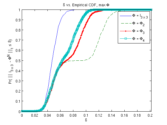
(d) non-ergodic attacks, $N=10^{5}$

Figure 3: Plot of empirical cdfs of $\|{\hat{\Phi}^{N}-I}\|_{1}$ obtained in the motivating example with the four relay manipulation maps corresponding to $\Phi_{1}=I,\Phi_{2}$, $\Phi_{3}$, and $\Phi_{4}$ respectively.

V-A1 I.i.d. attacks

To demonstrate the asymptotic maliciousness detection performance promised by Theorem 1, and to investigate the performance with finite observations, we performed simulations for four different manipulation maps which correspond to the relay randomly and independently switching its input symbol by symbol according to the conditional pmfs $p(v_{j}|u_{i})$ specified by the matrices

$$\Phi_{1}=I_{3\!\times\!3}, \Phi_{2}=\left(\begin{matrix}.99&.005&.005\\ .005&.99&.005\\ .005&.005&.99\end{matrix}\right),$$

$$\Phi_{3}=\left(\begin{matrix}.99&.005&0\\ .01&.99&.01\\ 0&.005&.99\\ \end{matrix}\right), \text{and~{}~{}}\Phi_{4}=\left(\begin{matrix}.99&0&0\\ .01&1&.01\\ 0&0&.99\\ \end{matrix}\right).$$ (5)

Obviously the case of $\Phi_{1}$ corresponds to a non-malicious relay and the other cases correspond to a malicious relay. The particular malicious $\Phi$’s were chosen to represent different ways a relay node may choose to attack. For the case of $\Phi_{2}$, the relay node changes $1$% of the symbols received without regards to whether or not this will make the manipulation obvious to the source nodes. In contrast, the attack of $\Phi_{3}$ is more reserved in what it will do. It can be seen that the relay’s manipulation can only be instantly detected by one of the source nodes at any given transmitted value. That is, the relay the relay switches $1$% of the received symbols in ways listed out in Table. I except those labeled with “Alice & Bob both detect.” Finally the attack of $\Phi_{4}$ is the most cautious and will only take an action that neither source node can recognize as manipulation without looking at multiple observations. For this case, the relay switches $2$% of the received symbols with values $0$ or $2$ to $1$. This corresponds to the “Not detected” outcomes in Table I. Note that $\|{\Phi^{N}-\Phi_{i}}\|_{1}\rightarrow 0$ in probability as $N\rightarrow\infty$ in each case. Hence property 1) of Corollary 1 applies for the case of $\Phi_{1}$ and property 4) applies for the cases of $\Phi_{2}$, $\Phi_{3}$, and $\Phi_{4}$.

In different simulation runs, we set $N=10^{3}$, $10^{4}$, and $10^{5}$. Five thousand trials were run in each simulation. The empirical cumulative distribution functions (cdfs) of $\|{\hat{\Phi}^{N}-I}\|_{1}$ obtained from the $5000$ trials for each simulation are plotted in Figs. 3a, 3b, and 3c for the cases of $N=10^{3}$, $10^{4}$, and $10^{5}$, respectively. For these three cases, the values of $\mu$ chosen in defining the estimator $\hat{\Phi}^{N}$ are $0.2$, $0.1$, and $0.05$, respectively. From Figs. 3b and 3c respectively with $N=10^{4}$ and $N=10^{5}$, as predicted by parts 1) and 4) of Corollary 1, the decision statistic $\|{\hat{\Phi}^{N}-I}\|_{1}$ succeeds in differentiating between the non-malicious case of $\Phi_{1}$ and the malicious cases of $\Phi_{2}$, $\Phi_{3}$, and $\Phi_{4}$ with very high confidence. For instance, by selecting the decision threshold at $\delta=0.065$ and $\delta=0.004$ respectively for the cases of $N=10^{4}$ and $N=10^{5}$, we are able to obtain very small miss and false alarm probabilities for detecting maliciousness of the relay. For $N=10^{3}$, we can see from Fig. 3a that there is still differentiation between the empirical cdfs obtained for the non-malicious and malicious cases. However the maliciousness differentiation confidence achieved is much weaker than the detectors with the larger value of $N$. This simulation exercise illustrates the fact that the decision statistic based on the maximum-norm estimator of (4), while is convenient for proving the asymptotic distinguishability result in Theorem 1, may not be a suitable choice for constructing a practical detector when the number of observations, $N$, is not large. Other more efficient finite-observation detectors may be needed.

V-A2 Non-ergodic attacks

To demonstrate part 2) of Corollary 1 with non-i.i.d attacks, we simulated a few non-ergodic attacks and considered again the decision statistic $\|{\hat{\Phi}^{N}-I}\|_{1}$. In these non-ergodic attacks, the relay decides whether or not to manipulate the symbols depending on if the checksum of all observed symbols is even or not. Conditioning on an even checksum, the relay manipulates the symbols i.i.d. according to $\Phi_{2}$, $\Phi_{3}$, and $\Phi_{4}$ as described in (5). Note that the for these attacks, $\lim_{N\rightarrow\infty}\Pr(\|{\Phi^{N}-I}\|_{1}>\delta)=0.5$ for all $\delta>0$.

The results for this simulation with $N=10^{5}$ and $\mu=0.01$ are plotted in Fig. 3d. From the figure, the first important note is that the empirical cdfs of the decision statistic exhibit staircase shapes with a step at $0.5$ as predicted by part 2) of Corollary 1. When the relay is being malicious, it is clear that by choosing $\delta=0.07$, we can again obtain small miss and false alarm probabilities for detecting maliciousness of the relay.

V-B Higher order example

$$A=\left(\begin{matrix}\frac{1}{3}&0&0\\ \frac{1}{3}&\frac{1}{3}&0\\ \frac{1}{3}&\frac{1}{3}&\frac{1}{3}\\ 0&\frac{1}{3}&\frac{1}{3}\\ 0&0&\frac{1}{3}\\ \end{matrix}\right),~{}B=\left(\begin{matrix}1&.5&0&0&0\\ 0&.5&.7&0&0\\ 0&0&.3&.5&0\\ 0&0&0&.5&1\\ \end{matrix}\right),~{}\Phi_{1}=I_{5\!\times\!5},~{}\Phi_{2}=\left(\begin{matrix}.99&.0025&.0025&.0025&.0025\\ .0025&.99&.0025&.0025&.0025\\ .0025&.0025&.99&.0025&.0025\\ .0025&.0025&.0025&.99&.0025\\ .0025&.0025&.0025&.0025&.99\\ \end{matrix}\right),$$

$$\Phi_{3}=\left(\begin{matrix}.99&\frac{.01}{3}&.0025&0&0\\ .005&.99&.0025&\frac{.01}{3}&0\\ .005&\frac{.01}{3}&.99&\frac{.01}{3}&.005\\ 0&\frac{.01}{3}&.0025&.99&.005\\ 0&0&.0025&\frac{.01}{3}&.99\\ \end{matrix}\right),\text{~{}and~{}}\Phi_{4}=\left(\begin{matrix}.985&0&0&0&0\\ .0075&.985&0&0&0\\ .0075&.015&1&.015&.0075\\ 0&0&0&.985&.0075\\ 0&0&0&0&.985\\ \end{matrix}\right).$$ (6)

(a) $(A,B)$ non-manipulable

(b) $(A,B)$ manipulable

Figure 4: Plot of empirical cdfs of $\|{\hat{\Phi}^{N}-I}\|_{1}$ for various i.i.d. attacks considered in Sections V-B and V-C.

Let us consider the addition channel as shown in Fig. 1 with both Alice and Bob choosing their source symbols uniformly over the ternary alphabet $\{0,1,2\}$ instead. Hence the input and output alphabets of Romeo is $\{0,1,2,3,4\}$ in this case. It is easy to verify that the corresponding $A$ matrix is given as in (6) on the next page. Furthermore, suppose that BC from Romeo back to Alice and Bob is not ideal. In particular, let us model the marginal BC from Romeo back to Alice by the matrix $B$ given in (6). Notice that this $B$ has a non-trivial right null space.

First we need to determine if the pair $(A,B)$ is non-manipulable. To do this, we used the Algorithm 1 presented in Section IV-B. In particular, we employed the linear programming solver linprog in the optimization toolbox in MATLAB to solve the linear program in step 2 of Algorithm 1. The optimal value returned was of the order of $10^{-16}$, which is close enough to $0$ for us to decide $(A,B)$ as non-manipulable. Thus again Theorem 1 and Corollary 1 apply to give that the decision statistic $\|{\hat{\Phi}^{N}-I}\|_{1}$ provides maliciousness detectability for this channel.

As in Section V-A1, we simulated i.i.d. attacks by Romeo. The four different $\Phi$’s shown in (6) were the cases that we considered in the simulation study. The attack of $\Phi_{1}$ corresponds to the case in which Romeo truthfully forwards the received symbols. For the attacks of $\Phi_{2}$, $\Phi_{3}$, and $\Phi_{4}$, Romeo alters $1$% of the symbols that it receives. Each of these three cases was once again chosen for a particular level of maliciousness as in Section V-A1. The case of $\Phi_{2}$ corresponds to an attack in which Romeo returns values that he knows will instantly guarantee detection. The attack of $\Phi_{3}$ only sends back values for which it is possible to not be instantly detected. Finally $\Phi_{4}$ corresponds to the case in which Romeo is the most cautious, and will not send back any symbol which is instantly detectable.

The empirical cdfs of $\|{\hat{\Phi}^{N}-I}\|_{1}$ obtained for the four different $\Phi_{i}$’s are plotted in Fig. 4a for the simulation run with $N=10^{5}$ and $\mu=0.05$. As before, by choosing a decision threshold at $\delta=0.07$ we can obtain very small miss and false alarm probabilities for detecting maliciousness of Romeo.

V-C Counter-example

To demonstrate the consequence of having a manipulable observation channel $(A,B)$, reconsider the ternary-input example of Section V-B with the marginal BC from Romeo back to Alice specified by the following matrix

$$B=\left(\begin{matrix}1&0&0&0&0\\ 0&.5&0&.3&.2\\ 0&0&.5&.2&.3\\ 0&.3&.2&.5&0\\ 0&.2&.3&0&.5\\ \end{matrix}\right).$$

To check whether $(A,B)$ is manipulable, Algorithm 1 was again employed. The optimal value of the linear program in step 2 obtained was $3$, thus alerting us that $(A,B)$ is manipulable. Indeed it can be readily check that for any $\psi\in(0,1]$, the matrix

$$\Upsilon=\left(\begin{matrix}0&0&0&0&0\\ 0&\psi&0&0&0\\ 0&0&\psi&0&-\psi\\ 0&-\psi&0&0&0\\ 0&0&-\psi&0&\psi\\ \end{matrix}\right),$$

is one that satisfies $B\Upsilon A=0$ required in Definition 5 to make $(A,B)$ manipulable. Therefore Theorem 1 tells us that maliciousness detectability is impossible for this channel.

As in Sections V-A1 and V-B, an i.i.d. attack with $\Phi_{2}=I-\Upsilon$ was simulated for $N=10^{5}$ and $\mu=0.05$. The value of $\psi=1$ was chosen in the simulation. This choice corresponds to an average of $\frac{5}{9}$ of the symbols are changed by Romeo. Clearly having this many symbols changed would be catastrophic in most practical communication systems, and is therefore undesirable. The empirical cdfs of the non-malicious case and the malicious case of $\Phi_{2}$ obtained from the simulation are plotted in Fig. 4b. It is clear from the figure that the cases for which Romeo is being malicious and not malicious are indistinguishable. Hence the severe attack of $\Phi_{2}$ can not be detected.

VI Proofs of Detectability Results

In order to prove the various results in Section IV, we will need to extend the notion of polarization of vectors given in Definition 4 to matrices:

Definition 6.

(Polarized matrices) Let $1\leq n\leq|U|$. For $b\geq 0$ and $0\leq\epsilon\leq b$, we say that a $n\!\times\!|U|$ matrix $\Upsilon$ is $(b,\epsilon)$-polarized if

$$\Upsilon_{i,j}\in\begin{cases}[b,\infty)&\mbox{~{}for~{}}j=i\\ (-\infty,\epsilon]&\mbox{~{}for~{}}j\neq i.\end{cases}$$

If, in addition, $\Upsilon_{i,j}=0$ for all $i,j=1,2,\ldots,n$ and $i\neq j$, we say that $\Upsilon$ is $(b,\epsilon)$-diagonal polarized.

Moreover, by saying a normalized $\Upsilon$ is in the left null space of $A$, we mean all rows of $\Upsilon$ are normalized vectors in the left null space of $A$.

In addition to the notion of polarized vectors and matrices, we will also employ the following generalization of linear dependence:

Definition 7.

($\epsilon_{s}$-dependent) A vector $\omega$ is $\epsilon_{s}$-dependent ($\epsilon_{s}\geq 0$) upon a set of vectors $\Upsilon_{1},\Upsilon_{2},\ldots,\Upsilon_{n}$ of the same dimension if there exists a set of coefficients $c_{1},c_{2},\ldots,c_{n}$ such that

$$\left\|\omega-\sum_{i=1}^{n}c_{i}\Upsilon_{i}\right\|_{1}\leq\epsilon_{s}.$$

With these definitions in place, we will first establish a few important and interesting properties of polarized vectors and matrices in the left and right null spaces of $A$ and $B$, respectively. In addition, we will show that the condition of the observation channel $(A,B)$ being non-manipulable is sufficient in guaranteeing the validity of these properties. Then we will apply some of these properties to bound the distance between an estimate of the attack channel and the true attack channel. The distance bound is employed to show that a decision statistic constructed from an attack channel estimator based on histogram estimation of node 1’s conditional pmf of its received symbols given its transmitted symbols provides the needed convergence properties in Theorem 1. The aforementioned properties of polarized vectors in the left null space of $A$ will also be used to prove Algorithm 2 and Theorem 2.

VI-A Properties concerning polarized vectors and matrices in null spaces of $A$ and $B$

Let us first study the left null space of $A$. The following simple lemma about normalized vectors in the left null space of $A$ is critical to many other results in this section:

Lemma 1.

Suppose that $\upsilon$ is a non-zero normalized $1\!\times\!|U|$ vector in the left null space of $A$. Then $\upsilon$ must contain at least one positive element and one negative element, and

$$\max_{i:\upsilon_{i}>0}\upsilon_{i} \geq a_{\min}$$

$$\min_{i:\upsilon_{i}<0}\upsilon_{i} \leq-a_{\min}.$$

Proof:

Write $a=\max_{i:\upsilon_{i}>0}\upsilon_{i}$ for convenience, and note that $a=0$ by definition if $\upsilon$ contains no positive element. Since $\upsilon$ is normalized, we have

$$\sum_{i:\upsilon_{i}\leq 0}|\upsilon_{i}|=1-\sum_{i:\upsilon_{i}>0}|\upsilon_{i}|\geq 1-a|U|.$$ (7)

Because $\upsilon$ is in the left null space of $A$, $\sum_{i}\upsilon_{i}A_{i,j}=0$ for all $j$. That implies

$$\sum_{i:\upsilon_{i}>0}\upsilon_{i}A_{i,j}=-\sum_{i:\upsilon_{i}\leq 0}\upsilon_{i}A_{i,j}=\sum_{i:\upsilon_{i}\leq 0}|\upsilon_{i}|A_{i,j}.$$ (8)

But, because $0\leq A_{i,j}\leq 1$, we can make the following inequality

$$\sum_{i:\upsilon_{i}>0}\upsilon_{i}A_{i,j}\leq\sum_{i:\upsilon_{i}>0}\upsilon_{i}\leq a|U|.$$

Substituting (8) back in, we get

$$a|U|\geq\sum_{i:\upsilon_{i}\leq 0}|\upsilon_{i}|A_{i,j}$$

which must hold for all $j$. Therefore,

$$a|U||X_{1}|\geq\sum_{j}\sum_{i:\upsilon_{i}\leq 0}|\upsilon_{i}|A_{i,j}\geq\sum_{i:\upsilon_{i}\leq 0}|\upsilon_{i}|A_{\min}$$

which causes a contradiction when $a=0$ since $A_{\min}>0$. Hence, $a$ must not be $0$, and $\upsilon$ must have at least one positive element. Further, by (7),

$$a|U||X_{1}|\geq A_{\min}\left(1-a|U|\right)$$

which gives the desired lower bound on $a$. The proof of existence of a negative element and the fact that the minimum negative element must be no larger than $-a_{\min}$ is similar. ∎

An immediate, but important later in proving Theorem 5, consequence of the lemma is the following observation:

Lemma 2.

Let $0<\epsilon\leq a_{\min}$. Suppose that $\omega$ is a normalized vector in the left null space of $A$ that is not $(a_{\min},\epsilon)$-polarized at $i$. Then there exists a $j\neq i$ such that $\omega_{j}\geq\epsilon$.

Proof:

Since $\omega$ is normalized, $\omega_{k}\geq a_{\min}$ for some $k$ by Lemma 1. If $k\neq i$, then we have the stated conclusion. Now suppose $k=i$. If $\omega_{j}<\epsilon$ for all $j\neq i$, then we obtain the contradictory conclusion that $\omega$ is $(a_{\min},\epsilon)$-polarized at $i$. ∎

Lemma 1 also implies the following two lemmas about normalized, diagonal polarized matrices in the left null space of $A$:

Lemma 3.

Let $a_{\min}\leq a\leq 1$ and $2\leq n\leq|U|$. Let $0\leq\epsilon_{s}<a_{\min}$, and $\epsilon$ and $\epsilon_{n-1}$ be two positive constants. Define

$$\epsilon^{\prime}_{n}=\frac{\epsilon+\epsilon_{s}}{a_{\min}-\epsilon_{s}}+(n-1)\frac{\epsilon+\epsilon_{n-1}+\epsilon_{s}+\epsilon_{s}\epsilon_{n-1}}{a(a_{\min}-\epsilon_{s})}.$$ (9)

Suppose that $\epsilon_{s}$, $\epsilon$, and $\epsilon_{n-1}$ are chosen small enough to satisfy $\epsilon^{\prime}_{n}<a_{\min}$. Furthermore, suppose that the left null space of $A$ contains a normalized, $(a,\epsilon_{n-1})$-diagonal polarized, $(n-1)\!\times\!|U|$ matrix and a normalized, $1\!\times\!|U|$ vector that is $(a,\epsilon)$-polarized at $n$, and is $\epsilon_{s}$-dependent on the rows of the matrix. Then the left null space of $A$ also contains a normalized, $1\!\times\!|U|$ vector that is $(a_{\min},\epsilon^{\prime})$-double polarized at $(m,n)$ for all $\epsilon^{\prime}_{n}\leq\epsilon^{\prime}<a_{\min}$, where $m<n$.

Proof:

Fix $\epsilon^{\prime}\in[\epsilon^{\prime}_{n},a_{\min})$. Let $\Upsilon$ and $\upsilon$ be the $(a,\epsilon_{n-1})$-diagonal polarized matrix and the $(a,\epsilon)$-polarized vector, respectively, given in the statement of the lemma. We will show that one row of $\Upsilon$ must be $(a_{\min},\epsilon^{\prime})$-double polarized at $(m,n)$, where $m<n$.

First, since $\upsilon$ is $\epsilon_{s}$-dependent upon the rows in $\Upsilon$, we know that there exists a set of coefficients $c_{1},c_{2},\ldots,c_{n-1}$ such that for any $j=1,2,\ldots,|U|$,

$$\upsilon_{j}-\epsilon_{s}\leq\sum_{i=1}^{n-1}c_{i}\Upsilon_{i,j}\leq\upsilon_{j}+\epsilon_{s}.$$ (10)

In particular, for $i=1,2,\ldots,n-1$, we have $\upsilon_{i}-\epsilon_{s}\leq c_{i}\Upsilon_{i,i}\leq\upsilon_{i}+\epsilon_{s}$. Using the facts that $\Upsilon_{i,i}\geq a$ and that $-1\leq\upsilon_{i}\leq\epsilon$, we can determine that

$$\frac{-1-\epsilon_{s}}{a}\leq c_{i}\leq\frac{\epsilon+\epsilon_{s}}{a}.$$ (11)

From Lemma 1, we know that there exists an index $m$ such that $\upsilon_{m}\leq-a_{\min}$. To proceed, we want to show that $m<n$, which we will do through contradiction. Obviously $m\neq n$. Suppose $m>n$ and consider (10) with $j=m$. Separating the terms with positive and negative $c_{i}$’s in the summation and using the upper bound in (10), we have

$$\sum_{i:c_{i}<0}|c_{i}|\Upsilon_{i,m} \geq-\upsilon_{m}-\epsilon_{s}+\sum_{i:c_{i}>0}c_{i}\Upsilon_{i,m}$$

$$\geq a_{\min}-\epsilon_{s}-(n-1)\frac{\epsilon+\epsilon_{s}}{a}$$ (12)

where the second inequality is obtained by using the upper bound on $c_{i}$ in (11). But because $m>n$, we have $\Upsilon_{i,m}\leq\epsilon_{n-1}$. Then by using the lower bound on $c_{i}$ in (11), we get $\sum_{i:c_{i}<0}|c_{i}|\Upsilon_{i,m}\leq(n-1)\epsilon_{n-1}\frac{1+\epsilon_{s}}{a}$. Thus we arrive at the conclusion that

$$(n-1)\epsilon_{n-1}\frac{1+\epsilon_{s}}{a}\geq a_{\min}-\epsilon_{s}-(n-1)\frac{\epsilon+\epsilon_{s}}{a},$$

which clearly violates the condition $\epsilon^{\prime}_{n}<a_{\min}$ in the statement of the lemma. Therefore $m<n$. Furthermore we have $c_{m}\Upsilon_{m,m}\leq\upsilon_{m}+\epsilon_{s}\leq-a_{\min}+\epsilon_{s}<0$, which implies $c_{m}<0$ and $|c_{m}|\geq a_{\min}-\epsilon_{s}$.

Similar to (12), we have, for $j>n$,

$$\sum_{i:c_{i}<0}|c_{i}|\Upsilon_{i,j} \geq-\upsilon_{j}-\epsilon_{s}+\sum_{i:c_{i}>0}c_{i}\Upsilon_{i,j}$$

$$\geq-\epsilon-\epsilon_{s}-(n-1)\frac{\epsilon+\epsilon_{s}}{a}$$ (13)

where the second inequality is due to the fact that $\upsilon_{j}\leq\epsilon$. Further separating the terms with positive and negative $\Upsilon_{i,j}$ in the sum on the left side of (13), for $j>n$, we have

$$\sum_{i:c_{i}<0,\Upsilon_{i,j}<0}|c_{i}||\Upsilon_{i,j}|$$ (14)

$$\leq \epsilon+\epsilon_{s}+(n-1)\frac{\epsilon+\epsilon_{s}}{a}+\sum_{i:c_{i}<0,\Upsilon_{i,j}>0}|c_{i}|\Upsilon_{i,j}$$

$$\leq \epsilon+\epsilon_{s}+(n-1)\frac{\epsilon+\epsilon_{n-1}+\epsilon_{s}+\epsilon_{s}\epsilon_{n-1}}{a}$$

where the second inequality results from the bound $\sum_{i:c_{i}<0,\Upsilon_{i,j}>0}|c_{i}|\Upsilon_{i,j}\leq(n-1)\epsilon_{n-1}\frac{1+\epsilon_{s}}{a}$, as shown above. Because $c_{m}<0$, we know from (14) that if $\Upsilon_{m,j}<0$, then $|c_{m}||\Upsilon_{m,j}|\leq\epsilon+\epsilon_{s}+(n-1)\frac{\epsilon+\epsilon_{n-1}+\epsilon_{s}+\epsilon_{s}\epsilon_{n-1}}{a}$. Further, by the above derived result that $|c_{m}|\geq a_{\min}-\epsilon_{s}$, we get

$$|\Upsilon_{m,j}|\leq\frac{\epsilon+\epsilon_{s}}{a_{\min}-\epsilon_{s}}+(n-1)\frac{\epsilon+\epsilon_{n-1}+\epsilon_{s}+\epsilon_{s}\epsilon_{n-1}}{a(a_{\min}-\epsilon_{s})}=\epsilon^{\prime}_{n},$$

if $\Upsilon_{m,j}<0$. Therefore, $|\Upsilon_{m,j}|\leq\epsilon^{\prime}$ for all $j>n$.

Combining all above results, we observe that $\Upsilon_{m,m}\geq a$, $|\Upsilon_{m,j}|\leq\epsilon^{\prime}<a_{\min}$ for $j>n$, and $\Upsilon_{m,j}=0$ for all other index values of $j$ except $n$. From Lemma 1, we must have $\Upsilon_{m,n}\leq-a_{\min}$. Thus $\Upsilon_{m}$ is $(a_{\min},\epsilon^{\prime})$-double polarized at $(m,n)$. ∎

Lemma 4.

Let $a_{\min}\leq a\leq 1$ and $2\leq n\leq|U|$. Let $0<\epsilon_{s}<a_{\min}$, and $\epsilon$ and $\epsilon_{n-1}$ be two positive constants. Define

$$\epsilon^{\prime\prime}_{n}=\frac{\epsilon_{n-1}}{a}+\frac{1}{a_{\min}a\epsilon_{s}}\left[\epsilon+(n-1)\frac{\epsilon+\epsilon_{n-1}}{a}\right].$$ (15)

Suppose that $\epsilon$ and $\epsilon_{n-1}$ are chosen small enough to satisfy $\epsilon^{\prime\prime}_{n}<a_{\min}$. Furthermore, suppose that the left null space of $A$ contains a normalized, $(a,\epsilon_{n-1})$-diagonal polarized, $(n-1)\!\times\!|U|$ matrix and a normalized, $1\!\times\!|U|$ vector that is $(a,\epsilon)$-polarized at $n$, and is not $\epsilon_{s}$-dependent on the rows of the matrix. Then the left null space of $A$ contains a normalized, $(a_{\min},\epsilon^{\prime\prime})$-diagonal polarized, $n\!\times\!|U|$ matrix, for all $\epsilon^{\prime\prime}_{n}\leq\epsilon^{\prime\prime}<a_{\min}$.

Proof:

Fix $\epsilon^{\prime\prime}\in[\epsilon^{\prime\prime}_{n},a_{\min})$. Let $\Upsilon$ and $\upsilon$ be the $(a,\epsilon_{n-1})$-diagonal polarized matrix and the $(a,\epsilon)$-polarized vector, respectively, given in the statement of the lemma. We will first construct a normalized, $1\!\times\!|U|$ vector $\hat{\upsilon}$ that is $(a_{\min},\epsilon^{\prime\prime})$-polarized at $n$ with the additional property that $\hat{\upsilon}_{j}=0$ for all $j=1,2,\ldots,n-1$. Then we apply elementary row operations and normalization to the rows of $[\Upsilon^{T}\hat{\upsilon}^{T}]^{T}$ to obtain the desired normalized, $n\!\times\!|U|$, $(a_{\min},\epsilon^{\prime\prime})$-diagonal polarized matrix.

First, set

$$\tilde{\upsilon}=\upsilon-\sum_{i=1}^{n-1}\frac{\upsilon_{i}}{\Upsilon_{i,i}}\Upsilon_{i}.$$

Because $\upsilon$ is not $\epsilon_{s}$-dependent upon the rows of $\Upsilon$, we must have $\|{\tilde{\upsilon}}\|_{1}>\epsilon_{s}$. Hence we can normalize $\tilde{\upsilon}$ to obtain $\hat{\upsilon}$, i.e., $\hat{\upsilon}=\tilde{\upsilon}/\|{\tilde{\upsilon}}\|_{1}$. Clearly, for $j<n$, $\tilde{\upsilon}_{j}=\upsilon_{j}-\frac{\upsilon_{j}}{\Upsilon_{j,j}}\Upsilon_{j,j}=0$, which implies $\hat{\upsilon}_{j}=0$. For $j>n$, write

$$\tilde{\upsilon}_{j}=\upsilon_{j}-\sum_{i:\upsilon_{i}>0}\frac{\upsilon_{i}}{\Upsilon_{i,i}}\Upsilon_{i,j}+\sum_{i:\upsilon_{i}<0}\frac{|\upsilon_{i}|}{\Upsilon_{i,i}}\Upsilon_{i,j}.$$ (16)

But since $\Upsilon_{i,i}\geq a$ and $\upsilon_{j}\leq\epsilon$ for $j>n$, we have

$$\sum_{i:\upsilon_{i}>0}\frac{\upsilon_{i}}{\Upsilon_{i,i}}\Upsilon_{i,j} \geq\sum_{i:\upsilon_{i}>0}\frac{\epsilon}{a}(-1)\geq-(n-1)\frac{\epsilon}{a}$$

$$\sum_{i:\upsilon_{i}<0}\frac{|\upsilon_{i}|}{\Upsilon_{i,i}}\Upsilon_{i,j} \leq\sum_{i:\upsilon_{i}<0}\frac{1}{a}\epsilon_{n-1}\leq(n-1)\frac{\epsilon_{n-1}}{a}.$$

Applying these two bounds to (16), we get, for $j>n$,

$$\tilde{\upsilon}_{j}\leq\epsilon+(n-1)\frac{\epsilon+\epsilon_{n-1}}{a},$$

which implies

$$\hat{\upsilon}_{j}\leq\frac{1}{\epsilon_{s}}\left[\epsilon+(n-1)\frac{\epsilon+\epsilon_{n-1}}{a}\right]\triangleq\varepsilon\leq\epsilon^{\prime\prime}_{n}.$$

Further, note that $\hat{\upsilon}$ is a normalized vector in the left null space of $A$. Hence by Lemma 1 and the fact that $\epsilon^{\prime\prime}_{n}<a_{\min}$, $\hat{\upsilon}_{n}\geq a_{\min}$. Therefore $\hat{\upsilon}$ is $(a_{\min},\varepsilon)$-polarized at $n$ with the additional property that $\hat{\upsilon}_{j}=0$ for $j<n$ as claimed.

Next, for $i=1,2,\ldots,n-1$, set

$$\tilde{\Upsilon}_{i}=\Upsilon_{i}-\frac{\Upsilon_{i,n}}{\hat{\upsilon}_{n}}\hat{\upsilon}.$$

Clearly, $\tilde{\Upsilon}_{i,n}=0$ and $\tilde{\Upsilon}_{i,j}=\Upsilon_{i,j}$ for $j<n$ by design. Thus $\|{\tilde{\Upsilon}_{i}}\|_{1}\geq a$. Again, we can normalize $\tilde{\Upsilon}_{i}$ to get $\hat{\Upsilon}_{i}=\tilde{\Upsilon}_{i}/\|{\tilde{\Upsilon}_{i}}\|_{1}$. Now, consider $j>n$,

$$\tilde{\Upsilon}_{i,j}=\Upsilon_{i,j}-\frac{\Upsilon_{i,n}}{\hat{\upsilon}_{n}}\hat{\upsilon}_{j}\leq\epsilon_{n-1}+\frac{\max\{\epsilon_{n-1},\varepsilon\}}{a_{\min}}=\epsilon_{n-1}+\frac{\varepsilon}{a_{\min}}$$

where the second inequality is due to $-1\leq\Upsilon_{i,n}\leq\epsilon_{n-1}$, $-1\leq\hat{\upsilon}_{j}\leq\varepsilon$, and $\hat{\upsilon}_{n}\geq a_{\min}$, and the last equality results from the fact that $|U|\epsilon_{s}<1$. Hence

$$\hat{\Upsilon}_{i,j}\leq\frac{\epsilon_{n-1}}{a}+\frac{\varepsilon}{a_{\min}a}=\epsilon^{\prime\prime}_{n}.$$

As discussed before, $\hat{\Upsilon}_{i,j}=0$ for all $i=1,2,\ldots,n-1$ and $j\neq i\leq n$. Hence, again using Lemma 1, we must have $\hat{\Upsilon}_{i,i}\geq a_{\min}$ since $\epsilon^{\prime\prime}<a_{\min}$. Finally, set $\hat{\Upsilon}_{n}=\hat{\upsilon}$. The matrix $\hat{\Upsilon}$ composed by using $\hat{\Upsilon}_{1},\hat{\Upsilon}_{2},\ldots,\hat{\Upsilon}_{n}$ as rows is the desired $(a_{\min},\epsilon^{\prime\prime})$-diagonal polarized matrix. ∎

To apply Lemmas 3 and 4, we need to the following lemma to select $\epsilon_{n}$:

Lemma 5.

Let $\epsilon_{s}$ and $\epsilon$ be two positive constants. Suppose that $2\leq n\leq|U|$. Define $\tilde{a}_{n-1}\triangleq a_{\min}^{2}\left(1+\frac{n-1}{a_{\min}}\right)^{-1}$. Set $\epsilon_{i}=\epsilon\left(\frac{2}{\tilde{a}_{n-1}\epsilon_{s}}\right)^{i-1}$ for $i=1,2,\ldots,n$. If

$$\epsilon_{s} <a_{\min}^{2}\tilde{a}_{n-1}\Bigg{\{}a_{\min}^{2}\left[1+\left(\frac{a_{\min}\tilde{a}_{n-1}}{2}\right)^{n-1}\right]$$

$$~{}~{}~{}~{}~{}~{}~{}~{}~{}~{}+(n-1)(1+a_{\min})\frac{\tilde{a}_{n-1}^{2}}{2}+a_{\min}\tilde{a}_{n-1}\Bigg{\}}^{-1}$$ (17)

and $\epsilon<a_{\min}\left(\frac{\tilde{a}_{n-1}\epsilon_{s}}{2}\right)^{n-1}$, then

1. $\epsilon_{1}\leq\epsilon_{2}\leq\cdots\leq\epsilon_{n}<a_{\min}$,

2. $\epsilon^{\prime}_{i}<a_{\min}$, $i=2,3,\ldots,n$,

3. $\epsilon^{\prime\prime}_{i}\leq\epsilon_{i}$, $i=2,3,\ldots,n$,

where $\epsilon^{\prime}_{i}$ and $\epsilon^{\prime\prime}_{i}$ are obtained from $\epsilon_{i-1}$ using the formulas given in (9) and (15) with $a\geq a_{\min}$, respectively.

Proof:

Part 1) is obvious from the construction. From (9) and 1), we have $\epsilon^{\prime}_{2}\leq\epsilon^{\prime}_{3}\leq\ldots\leq\epsilon^{\prime}_{n}$. Thus it suffices to show $\epsilon^{\prime}_{n}<a_{\min}$ when establishing 2). Indeed, note that $\epsilon_{n-1}<\frac{a_{\min}\tilde{a}_{n-1}}{2}\epsilon_{s}$, which together with (9) imply

$$\epsilon^{\prime}_{n} \leq\frac{1}{(a_{\min}-\epsilon_{s})\tilde{a}_{n-1}}\Bigg{\{}a_{\min}^{2}\left[\epsilon_{s}+a_{\min}\left(\frac{\tilde{a}_{n-1}\epsilon_{s}}{2}\right)^{n-1}\right]$$

$$~{}~{}~{}~{}~{}~{}~{}~{}~{}~{}~{}~{}~{}~{}~{}~{}~{}~{}~{}~{}~{}+(n-1)(1+\epsilon_{s})\frac{\tilde{a}_{n-1}^{2}\epsilon_{s}}{2}\Bigg{\}}$$

$$\leq\frac{\epsilon_{s}}{(a_{\min}-\epsilon_{s})\tilde{a}_{n-1}}\Bigg{\{}a_{\min}^{2}\left[1+\left(\frac{a_{\min}\tilde{a}_{n-1}}{2}\right)^{n-1}\right]$$

$$~{}~{}~{}~{}~{}~{}~{}~{}~{}~{}~{}~{}~{}~{}~{}~{}~{}~{}~{}~{}~{}+(n-1)(1+a_{\min})\frac{\tilde{a}_{n-1}^{2}}{2}\Bigg{\}}$$

$$<a_{\min}$$

where the last two inequalities result from the upper bound imposed on $\epsilon_{s}$ in the statement of the lemma.

Finally, it is easy to see from (15) that, for $i=2,3,\ldots,n$,

$$\epsilon^{\prime\prime}_{i}\leq\frac{1}{\tilde{a}_{n-1}\epsilon_{s}}(\epsilon_{i-1}+\epsilon)\leq\frac{2\epsilon_{i-1}}{\tilde{a}_{n-1}\epsilon_{s}}=\epsilon_{i}$$

where the second inequality is due to 1). ∎

Inductively applying Lemmas 3 and 4 with the choice of $\epsilon_{n}$ from Lemma 5, we obtain the following theorem:

Theorem 3.

Let $2\leq n\leq|U|$. Suppose that $\epsilon_{s}$, $\epsilon$, and $\epsilon_{1},\epsilon_{2},\ldots,\epsilon_{n}$ are chosen according to Lemma 5, and that the left null space of $A$ contains a normalized, $(a_{\min},\epsilon)$-polarized, $n\times|U|$ matrix. Then the left null space contains either a normalized, $(a_{\min},\epsilon^{\prime}_{i})$-double polarized, $1\!\times\!|U|$ vector for some $i=2,3,\ldots,n$, or a normalized, $(a_{\min},\epsilon_{n})$-diagonal polarized, $n\!\times\!|U|$ matrix. In the latter case, no row in the original $(a_{\min},\epsilon)$-polarized matrix can be $\epsilon_{s}$-dependent upon the other rows.

Proof:

Let $\Upsilon$ be the original $(a_{\min},\epsilon)$-polarized matrix in the left null space of $A$ given in the statement of the theorem. We will construct the desired $(a_{\min},\epsilon^{\prime}_{i})$-double polarized vector or $(a_{\min},\epsilon_{n})$-diagonal polarized matrix by inductively applying Lemmas 3 and 4 to the rows of $\Upsilon$.

First, set $\hat{\Upsilon}^{(1)}$ to be the first row of $\Upsilon$. The assumption of the theorem guarantees that $\hat{\Upsilon}^{(1)}$ satisfies that requirement of being a normalized, $(a_{\min},\epsilon_{1})$-diagonal polarized, $1\!\times\!|U|$ matrix in the left null space of $A$. Inductively, suppose that we have constructed, from the first $(i-1)$ rows of $\Upsilon$, the $(i-1)\!\times\!|U|$ normalized matrix $\hat{\Upsilon}^{(i-1)}$ that is $(a_{\min},\epsilon_{i-1})$-diagonal polarized and in the left null space of $A$. If the $i$th row of $\Upsilon$ is $\epsilon_{s}$-dependent on the rows of $\hat{\Upsilon}^{(i-1)}$ (i.e., the first $(i-1)$ rows of $\Upsilon$), then by Lemmas 3 and 5, there exists a normalized, $(a_{\min},\epsilon^{\prime}_{i})$-double polarized (at $(m,i)$ with $m<i$), $1\!\times\!|U|$ vector in the left null space of $A$. In this case, the induction process terminates. On the other hand, if the $i$th row of $\Upsilon$ is not $\epsilon_{s}$-dependent on the rows of $\Upsilon^{(i-1)}$, then Lemmas 4 and 5 together give an normalized $i\!\times\!|U|$ matrix $\hat{\Upsilon}^{(i)}$ that is $(a_{\min},\epsilon_{i})$-diagonal polarized and in the left null space of $A$. Also note that the rows of $\hat{\Upsilon}^{(i)}$ are in the span of the first $i$ rows of $\Upsilon$. The induction process continues until $i=n$. ∎

Theorem 3 leads to the following result that is critical to development in the next section:

Corollary 2.

Fix $2\leq n\leq|U|$, a positive $\epsilon_{s}$ satisfying (17), and $\frac{a_{\min}^{2}\epsilon_{s}}{(a_{\min}-\epsilon_{s})\tilde{a}_{n-1}}<\epsilon^{\prime}<a_{\min}$. Let the left null space of $A$ contain no normalized $(a_{\min},\epsilon^{\prime})$-double polarized, $1\!\times\!|U|$ vector. Then there exists a positive $\epsilon$ that if the left null space of $A$ contains a normalized, $(a_{\min},\epsilon)$-polarized $n\!\times\!|U|$ matrix, no row of such matrix can be $\epsilon_{s}$-dependent upon the other rows.

Proof:

For $i=1,2,\ldots,n-1$, choose $\epsilon_{i}=\epsilon\left(\frac{2}{\tilde{a}_{n-1}\epsilon_{s}}\right)^{i-1}$ as in Lemma 5. For any $\delta>0$, from (9), there exists a small enough $\epsilon$ such that $\epsilon^{\prime}_{n}\leq\frac{a_{\min}^{2}\epsilon_{s}}{(a_{\min}-\epsilon_{s})\tilde{a}_{n-1}}+\delta$. Choosing $\delta=\epsilon^{\prime}-\frac{a_{\min}^{2}\epsilon_{s}}{(a_{\min}-\epsilon_{s})\tilde{a}_{n-1}}$ and using part 1) of Lemma 5 give us $\epsilon^{\prime}_{2}\leq\epsilon^{\prime}_{3}\leq\ldots\leq\epsilon^{\prime}_{n}\leq\epsilon^{\prime}$. Now applying Theorem 3 gives us the desired result. ∎

The next lemma states that the observation channel $(A,B)$ being non-manipulable is sufficient for the condition of non-existence of any normalized $(a_{\min},\epsilon^{\prime})$-double polarized, $1\!\times\!|U|$ vector in the left null space of $A$ required in Corollary 2:

Lemma 6.

If $(A,B)$ is non-manipulable, then there exists a pair of constants $\epsilon_{s}$ and $\epsilon_{A}$ respectively satisfying

$$0<\epsilon_{s}<\min_{1\leq n\leq|U|-1}a_{\min}^{2}\tilde{a}_{n}\Bigg{\{}a_{\min}^{2}\left[1+\left(\frac{a_{\min}\tilde{a}_{n}}{2}\right)^{n}\right]$$

$$~{}~{}~{}~{}~{}~{}~{}~{}~{}~{}~{}~{}~{}~{}~{}~{}~{}~{}~{}~{}~{}~{}~{}~{}+n(1+a_{\min})\frac{\tilde{a}_{n}^{2}}{2}+a_{\min}\tilde{a}_{n}\Bigg{\}}^{-1},$$ (18)

$$\frac{a_{\min}^{2}\epsilon_{s}}{(a_{\min}-\epsilon_{s})\tilde{a}_{|U|-1}}<\epsilon_{A}<a_{\min},$$ (19)

such that the left null space of $A$ does not contain any normalized, $(a_{\min},\epsilon_{A})$-double polarized vectors.

Proof:

First we claim that the left null space of $A$ can not contain any normalized, $(a_{\min},0)$-double polarized vector if $(A,B)$ is non-manipulable. Indeed, suppose on the contrary that $\omega$ is a normalized vector in the left null space of $A$ that is $(a_{\min},0)$-double polarized at $(\alpha,\beta)$. Construct the $|U|\!\times\!1$ column vector $(\Upsilon_{\alpha}^{T})^{T}$ whose $\alpha$th element is $\omega_{\alpha}$, $\beta$th elements is $-\omega_{\alpha}$, and all other elements are zero. Similarly, construct the $|U|\!\times\!1$ column vector $(\Upsilon_{\beta}^{T})^{T}$ whose $\alpha$th element is $\omega_{\beta}$, $\beta$th elements is $-\omega_{\beta}$, and all other elements are zero. Then it is easy to check that $(\Upsilon_{\alpha}^{T})^{T}$ and $(\Upsilon_{\beta}^{T})^{T}$ are $(a_{\min},0)$-polarized at $\alpha$ and at $\beta$, respectively. Further, we also have, for all $l=1,2,\ldots,|X_{1}|$, $(\Upsilon_{\alpha}^{T})^{T}A_{\alpha,l}+(\Upsilon_{\beta}^{T})^{T}A_{\beta,l}=0$ because $\omega$ is in the left null space of $A$ and $\omega_{i}=0$ for all $i\neq\alpha$ or $\beta$. Hence $(A,B)$ is manipulable.

Next notice that both the set of normalized, $(a_{\min},0)$-double polarized vectors and the left null space of $A$ are closed sets. The former set is also bounded. As a result, if the left null space of $A$ does not contain any normalized, $(a_{\min},0)$-double polarized vectors, it must also not contain any normalized, $(a_{\min},\epsilon)$-double polarized vectors for all small enough positive $\epsilon$. Therefore by choosing $\epsilon_{s}$, satisfying (18), small enough, we obtain an $\epsilon_{A}$ that satisfies (19) and that the left null space of $A$ contains no $(a_{\min},\epsilon_{A})$-double polarized vectors. ∎

We now turn our attention to the right null space of $B$. The following result states that normalized vectors in the right null space of $B$ have similar properties of normalized vectors in the left null space of $A$ as described in Lemma 1:

Lemma 7.

The right null space of $B$ consists only of balanced vectors. Suppose that $\omega^{T}$ is a non-zero normalized $|U|\!\times\!1$ vector in the right null space of $B$. Let

$$b_{\min}\triangleq\frac{1}{|U|(|Y_{1}|+1)}.$$

Then

$$\max_{j:\omega_{j}>0}\omega_{j} \geq b_{\min}$$

$$\min_{j:\omega_{j}<0}\omega_{j} \leq-b_{\min}.$$

Proof:

Let $\omega^{T}$ be a vector in the right null space of $B$. Then

$$\sum_{i=1}^{|Y_{1}|}\sum_{j=1}^{|U|}B_{i,j}\omega_{j}=0.$$

Swapping the order of the two sums and using the fact that $\sum_{i=1}^{|Y_{1}|}B_{i,j}=1$, we get $\sum_{j=1}^{|U|}\omega_{j}=0$. Furthermore suppose $\omega^{T}$ is non-zero and normalized, it must then have at least one positive element and one negative element. Recognizing the preceding fact, we can employ essentially the same argument in the proof of Lemma 1 to show $\max_{j:\omega_{j}>0}\omega_{j}\geq b_{\min}$ and $\min_{j:\omega_{j}<0}\omega_{j}\leq-b_{\min}$. ∎

Based on Lemma 7, it is easy to check that the results from Lemma 3 to Corollary 2 all apply to $B^{T}$ with $a_{\min}$ replaced by $b_{\min}$ and $\tilde{a}_{n}$ defined in Lemma 5 replaced by $\tilde{b}_{n}\triangleq b_{\min}^{2}\left(1+\frac{n}{b_{\min}}\right)^{-1}$. That is, the above results are all applicable to normalized, polarized vectors and matrices in the right null space of $B$ with the corresponding modifications.

Finally, the next theorem states that non-manipulability of the observation channel $(A,B)$ guarantees the existence of a counterpart of Corollary 2 for the right null space of $B$ that is to be used in the proof of Theorem 5. To simplify notation in statement of the lemma, let $\mathcal{A}$ denote the set of all $|U|^{2}\!\times\!1$ column vectors of the form $\mathrm{vec}(\Upsilon A)$, where $\Upsilon$ is a $|U|\!\times\!|U|$ matrix whose $j$th column, for $j=1,2,\ldots,|U|$, is balanced and $(0,0)$-polarized at $j$, and $\|{\Upsilon}\|_{2}\leq 2|U|$. It is easy to check that the set $\mathcal{A}$ is closed, bounded, and convex. Let $\mathcal{\tilde{A}}$ denote the cone hull of $\mathcal{A}$. Then it can be readily checked that $\mathcal{\tilde{A}}$ is the set of vectors of the same form that make up $\mathcal{A}$ with the norm bound $\|{\Upsilon}\|_{2}\leq 2|U|$ removed.

Theorem 4.

Suppose that the right null space of $B$ is non-trivial, and the observation channel $(A,B)$ is non-manipulable. Then there exists a positive $\kappa$, which depends only on $A$ and $B$, satisfying the property that if $\Psi$ is a $|U|\!\times\!|U|$ matrix whose columns are vectors in the right null space of $B$ and $\|{\Psi}\|_{1}=1$, then there is a normalized vector $\upsilon$ simultaneously giving $\upsilon\,\mathrm{vec}(\Psi)\geq\kappa$ and $\upsilon\omega^{T}\leq 0$ for all $\omega^{T}\in\mathcal{A}$.

Proof:

Let $n=|U|-\mathrm{rank}(B)\geq 1$ be the dimension of the right null space of $B$. Let $\Xi$ be a $|U|\!\times\!n$ matrix whose columns form an orthonormal basis of the right null space of $B$. By flipping the polarities of the columns of $\Xi$ (i.e., the basis vectors), we obtain $2^{n}$ different bases for the right null space of $B$. Fix a normalized $\Psi$ with columns in the right null space of $B$. It is simple to check that $\frac{1}{|U|^{2}}\leq\|{\Psi}\|_{2}^{2}\leq 1$. For each $j=1,2,\ldots,|U|$, employing one, say $\Xi(j)$, among the $2^{n}$ bases above we can decompose $\Psi^{T}_{j}$ as $\Psi^{T}_{j}=\sum_{i=1}^{n}\left\{\Psi^{T}_{j}(\Xi(j)^{T}_{i})^{T}\right\}\,\Xi(j)^{T}_{i}$ with $\Psi^{T}_{j}(\Xi(j)^{T}_{i})^{T}\geq 0$ for all $i$. Let $\mathcal{B}$ be the convex hull of the set of vectors of the form $\mathrm{vec}(\Phi)$, where $\Phi$ is any $|U|\!\times\!|U|$ matrix such that $\Phi^{T}_{j}=\sum_{i=1}^{n}b_{i,j}\,\Xi(j)^{T}_{i}$ for $j=1,2,\ldots,|U|$ with $\frac{1}{|U|^{2}}\leq\sum_{i=1}^{n}\sum_{j=1}^{|U|}b_{i,j}^{2}\leq 1$ and $b_{i,j}\geq 0$ for $i$ and $j$. Obviously $\mathrm{vec}(\Psi)\in\mathcal{B}$. By geometric reasoning, $\mathcal{B}$ is a bounded set that does not contain the origin.

Since $(A,B)$ is non-manipulable, $\mathcal{\tilde{A}}$ must intersect trivially with the set of vectors of the form $\mathrm{vec}(\tilde{\Phi})$, where $\tilde{\Phi}$ is any $|U|\!\times\!|U|$ matrix whose columns are vectors in the right null space of $B$ (i.e., the intersection contains only the zero vector). Hence $\mathcal{B}$ and $\mathcal{\tilde{A}}$ are disjoint. Below we employ a slightly stronger version of the argument given in [27, pp. 48] to show that $\mathcal{B}$ and $\mathcal{\tilde{A}}$ can be strictly separated by a hyperplane that passes through the origin.

Given the above, we conclude that there exist $\mu_{a}^{T}\in\mathcal{\tilde{A}}$ and $\mu_{b}^{T}\in\mathcal{B}$ that achieve the minimum (positive) Euclidean distance between $\mathcal{\tilde{A}}$ and $\mathcal{B}$. Now let $\mu_{1}^{T}$ be an arbitrary vector in $\mathcal{\tilde{A}}$. Since $\mathcal{\tilde{A}}$ is a convex cone, $\mu_{a}^{T}+t(\alpha\mu_{1}^{T}-\mu_{a}^{T})\in\mathcal{\tilde{A}}$ for all $\alpha>0$ and $0<t\leq 1$. Hence $\|{\mu_{a}+t(\alpha\mu_{1}-\mu_{a})-\mu_{b}}\|_{2}^{2}\geq\|{\mu_{a}-\mu_{b}}\|_{2}^{2}$ for all $\alpha>0$ and $0<t\leq 1$, which (by letting $t\downarrow 0$) implies

$$(\mu_{a}-\mu_{b})\mu_{1}^{T}\geq\frac{1}{2\alpha}\left(\|{\mu_{a}-\mu_{b}}\|_{2}^{2}+\|{\mu_{a}}\|_{2}^{2}-\|{\mu_{b}}\|_{2}^{2}\right)$$ (20)

for all $\alpha>0$. Further, letting $\alpha\rightarrow\infty$ gives

$$(\mu_{a}-\mu_{b})\mu_{1}^{T}\geq 0.$$ (21)

Similarly, if $\mu_{2}^{T}$ be an arbitrary vector in $\mathcal{B}$, then $\mu_{b}^{T}+t(\mu_{2}^{T}-\mu_{b}^{T})\in\mathcal{B}$ by the convexity of $\mathcal{B}$. Then $\|{\mu_{b}+t(\mu_{2}-\mu_{b})-\mu_{a}}\|_{2}^{2}\geq\|{\mu_{a}-\mu_{b}}\|_{2}^{2}$ for all $0<t\leq 1$ gives

$$(\mu_{b}-\mu_{a})\mu_{2}^{T} \geq\frac{1}{2}\left(\|{\mu_{a}-\mu_{b}}\|_{2}^{2}+\|{\mu_{b}}\|_{2}^{2}-\|{\mu_{a}}\|_{2}^{2}\right)$$

$$\geq\|{\mu_{a}-\mu_{b}}\|_{2}^{2}$$ (22)

where the second inequality is due to the fact that $\|{\mu_{b}}\|_{2}^{2}-\|{\mu_{a}}\|_{2}^{2}\geq\|{\mu_{a}-\mu_{b}}\|_{2}^{2}$, which can in turn be verified by letting $\mu_{1}^{T}=0$ in (20) since $0\in\mathcal{A}$. Substituting $\mu_{1}=\omega$, $\mu_{2}^{T}=\mathrm{vec}(\Psi)$, $\upsilon=\frac{\mu_{b}-\mu_{a}}{\|{\mu_{b}-\mu_{a}}\|_{1}}$, and $\kappa_{\mathcal{B}}=\frac{\|{\mu_{b}-\mu_{a}}\|_{2}^{2}}{\|{\mu_{b}-\mu_{a}}\|_{1}}$ in (21) and (VI-A) almost establishes the lemma. The only technicality left to handle is that $\kappa_{\mathcal{B}}$ depends on $\Psi$. Fortunately, the dependence on $\Psi$ is only through the basis collection $\Xi(1),\Xi(2),\ldots,\Xi(|U|)$ that produces $\mathcal{B}$. Since there are only finitely many such collections to start with, the theorem is established by letting the required $\kappa$ to be the minimum among all the $2^{n|U|}$ $\kappa_{\mathcal{B}}$’s for the corresponding basis collections. ∎

VI-B Bounding attack channel estimation error

Recall that the attack channel matrix $\Phi^{N}$ is a $|U|\!\times\!|U|$ stochastic matrix. We consider below the stochastic matrix $\Gamma^{N}=B\Phi^{N}A$ as defined in (2), as well as estimates $\hat{\Phi}$ and $\hat{\Gamma}$ of $\Phi^{N}$ and $\Gamma^{N}$, respectively. In particular, we are interested in the estimators of $\Phi^{N}$ in $G_{\mu}(\hat{\Gamma})$ defined in Section III-D. For the purpose of proving Theorem 1 in the next section, the following result, which bounds the estimation error of estimators in $G_{\mu}(\hat{\Gamma})$, is important:

Theorem 5.

Let $\hat{\Gamma}$ be an estimate of $\Gamma^{N}$ based on the observation $(y_{1}^{N},x_{1}^{N})$. Let $\mu>0$ and $\hat{\Phi}\in G_{\mu}(\hat{\Gamma})$ be an estimate of $\Phi^{N}$. If $(A,B)$ is non-manipulable, then

$$\|{\Phi^{N}-\hat{\Phi}}\|_{1}\leq c_{1}\mu+c_{2}\,\|{\Gamma^{N}-\hat{\Gamma}}\|_{1}+c_{3}\,\|{\Phi^{N}-I}\|_{1}$$

for some positive constants $c_{1}$, $c_{2}$, and $c_{3}$ that depend only on $A$ and $B$.

Proof:

Let $\Xi_{A}$ and $\Xi_{B}$ denote the orthogonal projectors onto the left null space of $A$ and right null space of $B$, respectively. We decompose $\Phi^{N}-\hat{\Phi}$ into three components as below:

$$\Phi^{N}-\hat{\Phi} =\underbrace{(\Phi^{N}-\hat{\Phi})\Xi_{A}}_{\Theta^{A}\Psi^{A}}+\underbrace{\Xi_{B}(\Phi^{N}-\hat{\Phi})(I-\Xi_{A})}_{\Lambda^{B}}$$

$$~{}~{}~{}~{}~{}+\underbrace{(I-\Xi_{B})(\Phi^{N}-\hat{\Phi})(I-\Xi_{A})}_{\Lambda}$$ (23)

where the rows of $\Psi^{A}$ are normalized, and $\Theta^{A}$ is a $|U|\!\times\!|U|$ diagonal matrices whose strictly positive diagonal elements are the normalization constants for the rows of $\Psi^{A}$. Note that the rows of $\Psi^{A}$ are vectors in the left null space of $A$. Moreover the columns of $\Lambda^{B}$ are vectors in the right null space of $B$. Also note that we have assumed that $\Psi^{A}$ does not contain any all-zero rows without any loss of generality (see (24) below). Because the rows of $\Psi^{A}$ are normalized, we have from (23),

$$\|{\Phi^{N}-\hat{\Phi}}\|_{1}\leq\|{\Lambda^{B}+\Lambda}\|_{1}+\sum_{i=1}^{|U|}\Theta^{A}_{i,i}.$$ (24)

Thus it suffices to bound $\|{\Lambda^{B}+\Lambda}\|_{1}$ and the diagonal elements of $\Theta^{A}$.

We first bound the diagonal elements of $\Theta^{A}$. To do this, rewrite (23) as

$$I-\hat{\Phi}=I-\Phi^{N}+\Theta^{A}\Psi^{A}+\Lambda^{B}+\Lambda.$$ (25)

Because $\hat{\Phi}$ is a valid stochastic matrix, all diagonal elements of $I-\hat{\Phi}$ must be greater than or equal to $0$ and all off-diagonal elements must be less than or equal $0$. Thus (25) gives

$$\Theta^{A}_{i,i}\Psi^{A}_{i,j}\begin{cases}\geq-\|{I-\Phi^{N}}\|_{1}-\|{\Lambda^{B}+\Lambda}\|_{1}&\mbox{~{}if~{}}j=i\\ \leq\|{I-\Phi^{N}}\|_{1}+\|{\Lambda^{B}+\Lambda}\|_{1}&\mbox{~{}if~{}}j\neq i.\end{cases}$$ (26)

Now by Lemma 6, we have $\epsilon_{s}$ and $\epsilon_{A}$ respectively satisfy (18) and (19) such that the left null space of $A$ does not contain any $(a_{\min},\epsilon_{A})$-double polarized vectors. Hence we can choose a positive $\epsilon<a_{\min}$ so that the conclusion in Corollary 2 is valid for all $n=2,3,\ldots,|U|$. For this $\epsilon$, define

$$S_{\epsilon}=\{i:\big{|}\Psi^{A}_{i}\text{ is }(a_{\min},\epsilon)\text{-polarized at }i\}.$$

Let its cardinality be denoted by $n_{\epsilon}$.

We bound $\Theta^{A}_{i,i}$ for $i\notin S_{\epsilon}$ and $i\in S_{\epsilon}$ separately. First consider any $i\notin S_{\epsilon}$. Lemma 2 states that $[\Psi^{A}_{i}]_{j}\geq\epsilon$ for some $j\neq i$. Thus we have from (26) that

$$\Theta^{A}_{i,i}\leq\frac{\|{I-\Phi^{N}}\|_{1}+\|{\Lambda^{B}+\Lambda}\|_{1}}{\epsilon},$$ (27)

for all $i\notin S_{\epsilon}$.

Next we bound $\Theta^{A}_{i,i}$ for $i\in S_{\epsilon}$. If $n_{\epsilon}=0$, then there is nothing to do. Hence we assume $1\leq n_{\epsilon}\leq|U|$ below. Since each column of $\Lambda^{B}$ are in the right null space of $B$, it must be balanced according to Lemma 7. Moreover it is true that each column of $\Phi^{N}-\hat{\Phi}$ must also be balanced. As a result, (23) gives $\sum_{i=1}^{|U|}\Theta^{A}_{i,i}\Psi^{A}_{i,j}=-\sum_{i=1}^{|U|}\Lambda_{i,j}$ for $j=1,2,\ldots,|U|$. The triangle inequality then implies

$$\left|\sum_{i=1}^{|U|}\Theta^{A}_{i,i}\Psi^{A}_{i,j}\right|\leq\sum_{i=1}^{|U|}|\Lambda_{i,j}|.$$ (28)

Separating the sum on the left side of (28) into terms with index $i$ in and not in $S_{\epsilon}$, we have, for $j=1,2,\ldots,|U|$,

$$\left|\sum_{i\in S_{\epsilon}}\Theta^{A}_{i,i}\Psi^{A}_{i,j}\right|$$ (29)

$$\leq \sum_{i=1}^{|U|}|\Lambda_{i,j}|+\sum_{i\notin S_{\epsilon}}\Theta^{A}_{i,i}|\Psi^{A}_{i,j}|$$

$$\leq \sum_{i=1}^{|U|}|\Lambda_{i,j}|+\frac{|U|}{\epsilon}\left(\|{I-\Phi^{N}}\|_{1}+\|{\Lambda^{B}+\Lambda}\|_{1}\right)$$

where the second inequality is obtained by using (27) and the fact that the rows of $\Psi^{A}$ are normalized. For $2\leq n_{\epsilon}\leq|U|$, Corollary 2 suggests that for each $i\in S_{\epsilon}$,

$$\sum_{j=1}^{|U|}\left|\sum_{k\in S_{\epsilon}}\Theta^{A}_{k,k}\Psi^{A}_{k,j}\right| =\Theta^{A}_{i,i}\sum_{j=1}^{|U|}\left|\Psi^{A}_{i,j}+\sum_{k\in S_{\epsilon},k\neq i}\frac{\Theta^{A}_{k,k}}{\Theta^{A}_{i,i}}\Psi^{A}_{k,j}\right|$$

$$>\Theta^{A}_{i,i}\epsilon_{s}.$$ (30)

Note that the bound in (VI-B) is also trivially valid for the case of $n_{\epsilon}=1$ since $\epsilon_{s}<1$ and the rows of $\Psi^{A}$ are normalized. Substituting (29) into (VI-B), we obtain that for each $i\in S_{\epsilon}$,

$$\Theta^{A}_{i,i}<\frac{\|{\Lambda}\|_{1}}{\epsilon_{s}}+\frac{|U|^{2}}{\epsilon\epsilon_{s}}\left(\|{I-\Phi^{N}}\|_{1}+\|{\Lambda^{B}+\Lambda}\|_{1}\right)$$ (31)

Because $\epsilon_{s}\leq 1$, the upper bound on $\Theta^{A}_{i,i}$ for $i\in S_{\epsilon}$ is greater than the upper bound on $\Theta^{A}_{i,i}$ for $i\notin S_{\epsilon}$. Thus we can employ (31) as an upper bound for all $\Theta^{A}_{i,i}$’s. Note that the choices of $\epsilon_{A}$, $\epsilon_{s}$, and $\epsilon$ depend only $A$.

Next we proceed to bound $\|{\Lambda^{B}}\|_{1}$. Similar to before, write $\Lambda^{B}A=\theta^{B}\Psi^{B}$, where $\|{\Psi^{B}}\|_{1}=1$ and $\theta^{B}$ is the non-negative scaling factor. If the right null space of $B$ is trivial, $\Lambda^{B}=0$ and hence $\theta^{B}=0$. Otherwise, $\theta^{B}>0$. Without loss of generality, suppose the latter is true below. Because the linear mapping $(\cdot)A$ with domain restricted to the orthogonal complement of the left null space of $A$ is invertible, we have

$$\|{\Lambda^{B}}\|_{1}\leq c_{A}\|{\Lambda^{B}A}\|_{1}=c_{A}\theta^{B}$$ (32)

for some constant $c_{A}$ that depends only on $A$. Thus bounding $\theta^{B}$ is sufficient. To that end, right multiply both sides of (25) by $A$ to obtain

$$\underbrace{(I-\hat{\Phi})A}_{\Delta}=\theta^{B}\Psi^{B}+(I-\Phi^{N})A+\Lambda A.$$ (33)

Since $\hat{\Phi}$ is stochastic, $\mathrm{vec}(\Delta)\in\mathcal{A}$, where $\mathcal{A}$ is the set of $|U|^{2}\!\times\!1$ column vectors defined just right before Theorem 4 in Section VI-A. As $(A,B)$ is non-manipulable and the left-null space of $B$ is non-trivial, Theorem 4 guarantees the existence of a positive constant $\kappa$ and a normalized vector $\nu$ giving $\nu\,\mathrm{vec}(\Delta)\leq 0$ and $\nu\,\mathrm{vec}(\Psi^{B})\geq\kappa$. Note that $\kappa$ depends only on $A$ and $B$. Hence left-multiplying both sides of the vectorized version of (33) by $\nu$ yields

$$\theta^{B} \leq\frac{\left|\nu\,\{\mathrm{vec}((I-\Phi^{N})A)+\mathrm{vec}(\Lambda A)\}\right|}{\kappa}$$

$$\leq\frac{\|{(I-\Phi^{N})A}\|_{1}+\|{\Lambda A}\|_{1}}{\kappa}$$

$$\leq\frac{\sqrt{|U||X_{1}|^{2}}}{\kappa}\left(\|{I-\Phi^{N}}\|_{1}+\|{\Lambda}\|_{1}\right).$$

Applying this bound on $\theta^{B}$ back to (32), we obtain

$$\|{\Lambda^{B}}\|_{1}\leq\frac{c_{A}\sqrt{|U||X_{1}|^{2}}}{\kappa}\left(\|{I-\Phi^{N}}\|_{1}+\|{\Lambda}\|_{1}\right).$$ (34)

To complete the proof, we need to bound $\|{\Lambda}\|_{1}$. Note that there exists $\tilde{\Gamma}$ such that $B\hat{\Phi}A=\Pi_{B}\tilde{\Gamma}\Pi_{A}$ and $\|{\Pi_{B}(\tilde{\Gamma}-\hat{\Gamma})\Pi_{A}}\|_{1}\leq\mu$ since $\hat{\Phi}\in G_{\mu}(\hat{\Gamma})$. Then

$$B\Lambda A =B(\Phi^{N}-\hat{\Phi})A=\Gamma^{N}-\Pi_{B}\tilde{\Gamma}\Pi_{A}$$

$$=\Pi_{B}(\Gamma^{N}-\hat{\Gamma})\Pi_{A}+\Pi_{B}(\hat{\Gamma}-\tilde{\Gamma})\Pi_{A}$$ (35)

where the last equality is due to the fact that $\Gamma^{N}=\Pi_{B}\Gamma^{N}\Pi_{A}$. Note that the linear mapping $B(\cdot)A$ with domain restricted simultaneously to the orthogonal complements of the right null space of $B$ and left null space of $A$ is invertible. Combining this fact and (35), there exists a positive constant $c_{AB}$, which depends only on $A$ and $B$, such that

$$\|{\Lambda}\|_{1}\leq c_{AB}\left(\sqrt{|X_{1}||Y_{1}|}\cdot\|{\Gamma^{N}-\hat{\Gamma}}\|_{1}+\mu\right).$$ (36)

Finally, substituting (36), (34), and (31) back into (24), we obtain the desired bound on $\|{\Phi^{N}-\hat{\Phi}}\|_{1}$ given in the statement of the theorem with

$$c_{1} =\frac{c_{AB}|U|}{\epsilon_{s}}+c_{AB}\left(1+\frac{|U|^{3}}{\epsilon\epsilon_{s}}\right)\left(1+\frac{c_{A}\sqrt{|U||X_{1}|^{2}}}{\kappa}\right)$$

$$c_{2} =\sqrt{|X_{1}||Y_{1}|}\cdot c_{1}$$

$$c_{3} =\frac{|U|^{3}}{\epsilon\epsilon_{s}}+\frac{c_{A}\sqrt{|U||X_{1}|^{2}}}{\kappa}\left(1+\frac{|U|^{3}}{\epsilon\epsilon_{s}}\right).$$

∎

VI-C Proof of Theorem 1 and Corollary 1

VI-C1 Detectability

We prove the detectability portion of the theorem by showing that the sequence of decision statistics $\{D^{N}=\|{\hat{\Phi}^{N}-I}\|_{1}\}$, where $\hat{\Phi}^{N}$ is the estimator for the stochastic matrix $\Phi^{N}$ defined in (4), satisfies the two desired properties if the observation channel $(A,B)$ is non-manipulable.

To that end, first note that $\hat{\Phi}^{N}$ is obtained from the conditional histogram estimator $\hat{\Gamma}^{N}$ of the stochastic matrix $\Gamma^{N}$ defined in (3). We need the following convergence property of the sequence $\{\hat{\Gamma}^{N}\}$:

Lemma 8.

$\|{{\Gamma}^{N}-\hat{\Gamma}^{N}}\|_{1}\rightarrow 0$ in probability as $N$ approaches infinity.

Proof:

First, define the $|U|\!\times\!|X_{1}|$ stochastic matrix $\Omega^{N}$ by its $(i,j)$th element as

$$\Omega^{N}_{i,j}\triangleq\frac{\pi^{N}(v_{i},x_{1,j})}{\pi^{N}(x_{1,j})}.$$ (37)

For any $\mu>0$, it is clear that

$$\Pr\left(\|{{\Gamma}^{N}-\hat{\Gamma}^{N}}\|_{1}>\mu\right)$$ (38)

$$\leq \Pr\left(\|{B\Omega^{N}-\hat{\Gamma}^{N}}\|_{1}>\frac{\mu}{2}\right)+\Pr\left(\|{B\Omega^{N}-{\Gamma}^{N}}\|_{1}>\frac{\mu}{2}\right)$$

$$\leq \Pr\left(\|{B\Omega^{N}-\hat{\Gamma}^{N}}\|_{1}>\frac{\mu}{2}\right)$$

$$+\Pr\left(\|{\Omega^{N}-\Phi^{N}A}\|_{1}>\frac{\mu}{2\sqrt{|X_{1}||Y_{1}|}\cdot\|{B}\|_{2}}\right).$$

Thus the lemma is proved if we can show that the two probabilities on the right hand side of (38) converge to $0$ as $N$ approaches infinity.

To that end, notice first that

$$\|{B\Omega^{N}-\hat{\Gamma}^{N}}\|_{1}$$

$$= \sum_{i=1}^{|Y_{1}|}\sum_{j=1}^{|X_{1}|}|[B\Omega^{N}]_{i,j}-\hat{\Gamma}^{N}_{i,j}|$$

$$\leq \sum_{i=1}^{|Y_{1}|}\sum_{j=1}^{|X_{1}|}\sum_{k=1}^{|U|}\Big{|}\underbrace{p(y_{1,i}|v_{k})\frac{\pi^{N}(v_{k},x_{1,j})}{\pi^{N}(x_{1,j})}-\frac{\pi^{N}(y_{1,i},v_{k},x_{1,j})}{\pi^{N}(x_{1,j})}}_{H_{i,j,k}}\Big{|}$$

where the inequality above is due to the fact that $\pi^{N}(y_{1,i},x_{1,j})=\sum_{k}\pi^{N}(y_{1,i},v_{k},x_{1,j})$. This implies that

$$\Pr\left(\|{B\Omega^{N}-\hat{\Gamma}^{N}}\|_{1}>\frac{\mu}{2}\right)$$ (39)

$$\leq \sum_{i=1}^{|Y_{1}|}\sum_{j=1}^{|X_{1}|}\sum_{k=1}^{|U|}\Pr\left(|H_{i,j,k}|>\frac{\mu}{2|U||X_{1}||Y_{1}|}\right).$$

But for any $i$, $j$, and $k$,

$$\Pr\left(|H_{i,j,k}|>\frac{\mu}{2|U||X_{1}||Y_{1}|}\right)\leq\frac{4|U|^{2}|X_{1}|^{2}|Y_{1}|^{2}}{\mu^{2}}E\left[H_{i,j,k}^{2}\right]$$

$$\leq \frac{4|U|^{2}|X_{1}|^{2}|Y_{1}|^{2}}{\mu^{2}}\left\{\Pr(x^{N}_{1}\notin T^{N}_{[X_{1}],\delta})+E_{[X_{1}],\delta}[H_{i,j,k}^{2}]\right\},$$

where $E_{[X_{1}],\delta}[\cdot]$ denotes that conditional expectation $E[\cdot|x^{N}_{1}\in T^{N}_{[X_{1}],\delta}]$. Further, for any small enough positive $\delta$,

$$E_{[X_{1}],\delta}[H_{i,j,k}^{2}]$$ (43)

$$\leq \frac{E_{[X_{1}],\delta}\left[(p(y_{1,i}|v_{k})\pi^{N}(v_{k},x_{1,j})-\pi^{N}(y_{1,i},v_{k},x_{1,j}))^{2}\right]}{N^{2}(p(x_{1,j})-\delta)^{2}}$$

$$= \frac{\sum_{n=1}^{N}E_{[X_{1}],\delta}\left[\begin{array}[]{l}E\left[(p(y_{1,i}|v_{k})-1_{n}(y_{1,i}))^{2}|v^{N},x_{1}^{N}\right]\\ ~{}\cdot 1_{n}(v_{k},x_{1,j})\end{array}\right]}{N^{2}(p(x_{1,j})-\delta)^{2}}$$

$$\leq \frac{p(y_{1,i}|v_{k})}{N(p(x_{1,j})-\delta)^{2}}$$ (44)

where the equality on the third line above results from the fact that $p(y^{N}_{1}|v^{N},x^{N}_{1})=p(y^{N}_{1}|v^{N})$ and the elements of $y^{N}_{1}$ are conditionally independent given $v^{N}$. Combining (44) and the well known fact, for example see [26, Theorem 6.2], that $\Pr(x^{N}_{1}\notin T^{N}_{[X_{1}],\delta})\rightarrow 0$ as $N\rightarrow\infty$, we get from (LABEL:e:PrH) that $\Pr\left(|H_{i,j,k}|>\frac{\mu}{2|U||X_{1}||Y_{1}|}\right)\rightarrow 0$ as $N\rightarrow\infty$. Using (39), we further get $\Pr\left(\|{B\Omega^{N}-\hat{\Gamma}^{N}}\|_{1}>\frac{\mu}{2}\right)\rightarrow 0$ as $N\rightarrow\infty$.

Next, note that we can rewrite (37) as

$$\Omega^{N}_{i,j} =\frac{\pi^{N}(u_{i},x_{1,j})}{\pi^{N}(x_{1,j})}-\sum_{k\neq i}\frac{\pi^{N}(v_{k},u_{i},x_{1,j})}{\pi^{N}(x_{1,j})}$$

$$~{}~{}~{}~{}+\sum_{k\neq i}\frac{\pi^{N}(v_{i},u_{k},x_{1,j})}{\pi^{N}(x_{1,j})}.$$

Similarly, we have

$$\left[\Phi^{N}A\right]_{i,j} =p(u_{i}|x_{1,j})-\sum_{k\neq i}\frac{\pi^{N}(v_{k},u_{i})}{\pi^{N}(u_{i})}p(u_{i}|x_{1,j})$$

$$~{}~{}~{}~{}+\sum_{k\neq i}\frac{\pi^{N}(v_{i},u_{k})}{\pi^{N}(u_{k})}p(u_{k}|x_{j}).$$

Let

$$H^{1}_{i,j} =\frac{\pi^{N}(u_{i},x_{1,j})}{\pi^{N}(x_{1,j})}-p(u_{i}|x_{1,j})$$

$$H^{2}_{i,j} =\sum_{k\neq i}\frac{\pi^{N}(v_{k},u_{i},x_{1,j})}{\pi^{N}(x_{1,j})}-\frac{\pi^{N}(v_{k},u_{i})}{\pi^{N}(u_{i})}p(u_{i}|x_{1,j})$$

$$H^{3}_{i,j} =\sum_{k\neq i}\frac{\pi^{N}(v_{i},u_{k},x_{1,j})}{\pi^{N}(x_{1,j})}-\frac{\pi^{N}(v_{i},u_{k})}{\pi^{N}(u_{k})}p(u_{k}|x_{1,j}).$$

Then we have, for each $i$ and $j$,

$$\Pr\left(\left|\Omega^{N}_{i,j}-[\Phi^{N}A]_{i,j}\right|>\frac{\mu}{2|U||X_{1}|\sqrt{|X_{1}||Y_{1}|}\cdot\|{B}\|_{2}}\right)$$ (45)

$$\leq \sum_{l=1}^{3}\Pr\left(|H^{l}_{i,j}|>\frac{\mu}{6|U||X_{1}|\sqrt{|X_{1}||Y_{1}|}\cdot\|{B}\|_{2}}\right).$$

By employing the fact that $p(x^{N}_{1}|u^{N},v^{N})=p(x^{N}_{1}|u^{N})$ and the conditional independence of the elements of $u^{N}$ given $x^{N}_{1}$, each of the three probabilities on the right hand side of (45) can be shown to converge to $0$ as $N$ approaches infinity by using typicality arguments similar to the one that shows $\Pr\left(|H_{i,j,k}|>\frac{\mu}{2|U||X_{1}||Y_{1}|}\right)\rightarrow 0$ above. Thus, the probability on the left hand side of (45) also converges to $0$ as $N$ approaches infinity. Finally,

$$\Pr\left(\|{\Omega^{N}-\Phi^{N}A}\|_{1}>\frac{\mu}{2\sqrt{|X_{1}||Y_{1}|}\cdot\|{B}\|_{2}}\right)$$

$$\leq \sum_{i=1}^{|U|}\sum_{j=1}^{|X_{1}|}\Pr\Bigg{(}\left|\Omega^{N}_{i,j}-[\Phi^{N}A]_{i,j}\right|$$

$$~{}~{}~{}~{}~{}~{}~{}~{}~{}~{}~{}~{}~{}~{}~{}~{}~{}~{}>\frac{\mu}{2|U||X_{1}|\sqrt{|X_{1}||Y_{1}|}\cdot\|{B}\|_{2}}\Bigg{)}$$

$$\rightarrow 0$$

as $N\rightarrow\infty$. ∎

Now we proceed to show detectability in Theorem 1. For any fixed $\mu>0$, choose $\hat{\Phi}^{N}$ according to (4). It is clear from the definition of $G_{\mu}(\hat{\Gamma}^{N})$ in Section III-D that $\Phi^{N}\in G_{\mu}(\hat{\Gamma}^{N})$ whenever $\|{\Gamma^{N}-\hat{\Gamma}^{N}}\|_{1}\leq\frac{\mu}{\sqrt{|X_{1}||Y_{1}|}}$. Thus Lemma 8 implies that $\Pr(\Phi^{N}\in G_{\mu}(\hat{\Gamma}^{N}))\rightarrow 1$ as $N\rightarrow\infty$, and hence the probability that $G_{\mu}(\hat{\Gamma}^{N})$ is non-empty approaches $1$. We employ this property below to show that the sequence of decision statistics $\{\|{\hat{\Phi}^{N}-I}\|_{1}\}$ satisfies both Properties 1 and 2 stated in the theorem.

To show Property 1 of Theorem 1, first note that

$$\Pr\left(\|{\hat{\Phi}^{N}-I}\|_{1}>\delta~{}\bigcap~{}\|{\Phi^{N}-I}\|_{1}>\delta\right)$$ (46)

$$\geq \Pr\Big{(}\Phi^{N}\in G_{\mu}(\hat{\Gamma}^{N})~{}\bigcap~{}\|{\hat{\Phi}^{N}-I}\|_{1}>\delta$$

$$~{}~{}~{}~{}~{}~{}~{}\bigcap~{}\|{\Phi^{N}-I}\|_{1}>\delta\Big{)}$$

$$= \Pr\left(\Phi^{N}\in G_{\mu}(\hat{\Gamma}^{N})~{}\bigcap~{}\|{\Phi^{N}-I}\|_{1}>\delta\right)$$

$$\geq \Pr(\|{\Phi^{N}-I}\|_{1}>\delta)-\Pr(\Phi^{N}\notin G_{\mu}(\hat{\Gamma}^{N}))$$

where the equality on the third line is due to the definition of $\hat{\Phi}^{N}$ in (4). Hence, if $\limsup_{N\rightarrow\infty}\Pr(\|{\Phi^{N}-I}\|_{1}>\delta)>0$, (46) implies

$$\limsup_{N\rightarrow\infty}\Pr(\|{\hat{\Phi}^{N}-I}\|_{1}>\delta~{}|~{}\|{\Phi^{N}-I}\|_{1}>\delta)=1.$$

To show Property 2 of Theorem 1, consider the constants $c_{1}$, $c_{2}$, and $c_{3}$ given in Theorem 5. Let $c=2+c_{3}$. By choosing $0<\mu\leq\frac{\delta}{2c_{1}}$ and making use of Theorem 5, it is easy to check that

$$\Pr\left(\|{\Gamma^{N}-\hat{\Gamma}^{N}}\|_{1}\leq\frac{\mu}{\sqrt{|X_{1}||Y_{1}|}}~{}\bigcap~{}\|{\Phi^{N}-I}\|_{1}\leq\delta\right)$$

$$~{}~{}\leq \Pr\left(\|{\hat{\Phi}^{N}-I}\|_{1}\leq c\delta~{}\bigcap~{}\|{\Phi^{N}-I}\|_{1}\leq\delta\right)$$

which in turn implies

$$\Pr\left(\|{\hat{\Phi}^{N}-I}\|_{1}>c\delta~{}\bigcap~{}\|{\Phi^{N}-I}\|_{1}\leq\delta\right)$$ (47)

$$\leq \Pr\left(\|{\Gamma^{N}-\hat{\Gamma}^{N}}\|_{1}>\frac{\mu}{\sqrt{|X_{1}||Y_{1}|}}\right).~{}~{}~{}~{}~{}~{}~{}~{}~{}~{}~{}~{}~{}$$

Hence by Lemma 8, if $\liminf_{N\rightarrow\infty}\Pr(\|{\Phi^{N}-I}\|_{1}\leq\delta)>0$, (47) gives

$$\lim_{N\rightarrow\infty}\Pr(\|{\hat{\Phi}^{N}-I}\|_{1}>c\delta~{}|~{}\|{\Phi^{N}-I}\|_{1}\leq\delta)=0.$$

VI-C2 Corollary 1

Now we can use the results above to prove Corollary 1 by showing the sequence of decision statistics $\{\|{\hat{\Phi}^{N}-I}\|_{1}\}$ satisfies the four stated properties under the corresponding special cases:

$\|{\Phi^{N}-I}\|_{1}\rightarrow 0$ in probability

Since

$$\Pr(\|{\hat{\Phi}^{N}-I}\|_{1}>\delta)$$

$$\leq \Pr\left(\|{\hat{\Phi}^{N}-I}\|_{1}>\delta~{}\Big{|}~{}\|{\Phi^{N}-I}\|_{1}\leq\frac{\delta}{c}\right)$$

$$~{}\cdot\Pr\left(\|{\Phi^{N}-I}\|_{1}\leq\frac{\delta}{c}\right)+\Pr\left(\|{\Phi^{N}-I}\|_{1}>\frac{\delta}{c}\right)$$

for any $\delta>0$, Property 2 of Theorem 1 implies $\lim_{N\rightarrow\infty}\Pr(\|{\hat{\Phi}^{N}-I}\|_{1}>\delta)=0$.

$\|{\Phi^{N}-I}\|_{1}\nrightarrow 0$ in probability

If $\limsup_{N\rightarrow\infty}\Pr(\|{\Phi^{N}-I}\|_{1}>\delta)=0$, then there is nothing to show. Otherwise, Lemma 8 and (46) give $\limsup_{N\rightarrow\infty}\Pr(\|{\hat{\Phi}^{N}-I}\|_{1}>\delta)\geq\limsup_{N\rightarrow\infty}\Pr(\|{\Phi^{N}-I}\|_{1}>\delta)$.

$\|{\Phi^{N_{M}}-\Phi}\|_{1}\rightarrow 0$ in probability and $\Phi\neq I$

Note that there exists $\delta>0$ such that $\limsup_{N\rightarrow\infty}\Pr(\|{\Phi^{N}-I}\|_{1}>\delta)=1$ in this case. For any such $\delta$, Property 2 just above implies the required result.

$\|{\Phi^{N}-\Phi}\|_{1}\rightarrow 0$ in probability and $\Phi\neq I$

In this case, there exists $\delta>0$ such that $\lim_{N\rightarrow\infty}\Pr(\|{\Phi^{N}-I}\|_{1}>\delta)=1$. Using Lemma 8 and (46) gives the desired result for any such $\delta$.

VI-C3 Converse

Recall that $x_{1}^{N}$ and $y_{1}^{N}$ are the sequences of symbols transmitted and received by node 1 at time instants $1,2,\ldots,N$ and $N+1,N+2,\ldots,2N$, respectively. Let $D^{N}=D^{N}(x_{1}^{N},y_{1}^{N})$ be the $N$th decision statistic in the sequence, assumed to exist in the statement of Theorem 1, that satisfies Properties 1 and 2. Suppose that there exists a stochastic $\Phi^{\prime}\neq I$ such that $B\Phi^{\prime}A=BA\triangleq\Gamma$.

For the identity relay manipulation map, i.e., $\phi^{N}(u^{N})=u^{N}$, it is easy to check that $p(v^{n}|u^{n})=\prod_{n=1}^{N}I_{\chi_{n}(v^{N}),\chi_{n}(u^{N})}$, $\Phi^{N}=I$, and $p(y^{N}|x^{N})=\prod_{n=1}^{N}\Gamma_{\chi_{n}(y_{1}^{N}),\chi_{n}(x_{1}^{N})}$. Since $\Phi^{N}=I$ for all $N$, we have for every $\delta>0$,

$$\sum_{(x_{1}^{N},y_{1}^{N}):D^{N}(x_{1}^{N},y_{1}^{N})>\delta}\underbrace{\left[\prod_{i=n}^{N}\Gamma_{\chi_{n}(y_{1}^{N}),\chi_{n}(x_{1}^{N})}\cdot p(x_{1,\chi_{n}(x_{1}^{N})})\right]}_{q(y_{1}^{N},x_{1}^{N})}$$ (48)

$$= \Pr(D^{N}>\delta)$$

$$= \Pr\left(D^{N}>\delta~{}\Big{|}~{}\|{\Phi^{N}-I}\|_{1}\leq\frac{\delta}{c}\right)$$

$$\rightarrow 0$$

where the convergence on the last line is due to the assumption that Property 2 of Theorem 1 holds, and $c$ is the constant described in the property.

Consider now the random relay manipulation map that results in $p(v^{n}|u^{n})=\prod_{n=1}^{N}\Phi^{\prime}_{\chi_{n}(v^{N}),\chi_{n}(u^{N})}$. For this random manipulation map, it is again easy to check that $p(y^{N}|x^{N})=\prod_{n=1}^{N}\Gamma_{\chi_{n}(y_{1}^{N}),\chi_{n}(x_{1}^{N})}$, which is a consequence of the assumption that $B\Phi^{\prime}A=\Gamma$, and $\|{\Phi^{N}-\Phi^{\prime}}\|_{1}\rightarrow 0$ in probability. Since $\Phi^{\prime}\neq I$, there exists a $\delta>0$ such that $\lim_{N\rightarrow\infty}\Pr(\|{\Phi^{N}-I}\|_{1}>\delta)=1$. For this $\delta$,

$$\limsup_{N\rightarrow\infty}\sum_{(x_{1}^{N},y_{1}^{N}):D^{N}(x_{1}^{N},y_{1}^{N})>\delta}q(y_{1}^{N},x_{1}^{N})$$ (49)

$$= \limsup_{N\rightarrow\infty}\Pr(D^{N}>\delta)$$

$$\geq \limsup_{N\rightarrow\infty}\Pr\left(D^{N}>\delta~{}\Big{|}~{}\|{\Phi^{N}-I}\|_{1}>\delta\right)$$

$$~{}\cdot\lim_{N\rightarrow\infty}\Pr(\|{\Phi^{N}-I}\|_{1}>\delta)$$

$$= 1$$

where the equality on the last line is due to the assumption that Property 1 of Theorem 1 holds. The conclusions in (48) and (49) are clearly in conflict and can not be simultaneously true. Therefore there can not exist a stochastic $\Phi^{\prime}\neq I$ such that $B\Phi^{\prime}A=BA$ and Properties 1 and 2 hold.

To complete the proof of the converse, we need to show the existence of a stochastic $\Phi^{\prime}\neq I$ with the property that $B\Phi^{\prime}A=BA$ when the observation channel $(A,B)$ is manipulable. To that end, first note that the manipulability of $(A,B)$ implies the existence of a non-zero $\Upsilon$ with the property that all columns of $\Upsilon A$ are in the right null space of $B$. In addition, $(\Upsilon^{T}_{j})^{T}$ is balanced and $(0,0)$-polarized at $j$, for each $j=1,2,\ldots,|U|$. Let $\tilde{\Upsilon}=\frac{\Upsilon}{\max_{j}\Upsilon_{j,j}}$ and $\Phi^{\prime}=I-\tilde{\Upsilon}$. It then easy to check that this $\Phi^{\prime}$ is a valid stochastic matrix, $\Phi^{\prime}\neq 1$, and $B\Phi^{\prime}A=BA$.

VI-D Justification for Algorithms 1 and 2

Algorithm 1

Let $\Upsilon$ be a $|U|\!\times\!|U|$ matrix-valued variable and $s$ be a $|U|\!\times\!1$ vector-valued variable. Consider the following convex optimization problem:

$$\min_{s,\Upsilon}~{}\min\{-s_{1},-s_{2},\ldots,-s_{|U|}\}$$

$$\mathrm{\;subject\ to}$$

$$\quad B\Upsilon A=0$$

$$\quad\sum_{k=1}^{|U|}\Upsilon_{k,l}=0 l=1,2,\ldots,|U|,$$

$$\quad s_{k}-\Upsilon_{k,k}\leq 0 k=1,2,\ldots,|U|,$$

$$\quad\Upsilon_{k,k}-1\leq 0 k=1,2,\ldots,|U|,$$

$$\quad\Upsilon_{k,l}\leq 0 k\neq l=1,2,\ldots,|U|.$$ (50)

It is clear that the optimal value of (50) is attained and lies inside the interval $[-1,0]$. This further implies that $(A,B)$ is non-manipulable if and only if the optimal value of (50) is $0$.

Now, let $\Omega$ and $\nu$ be the $|X_{1}|\!\times\!|Y_{1}|$ matrix-valued and $|U|\!\times\!1$ vector-valued Lagrange multipliers for the equality constraints shown in the third and fourth lines of (50). Further, let $\Lambda$ be the $|U|\!\times\!|U|$ matrix-valued Lagrange multiplier matrix. The diagonal elements of $\Lambda$ correspond to the inequality constraints shown in the fifth line of (50), while the off-diagonal elements correspond to the inequality constraints shown in the last line of (50). At last, let $\nu$ be the $|U|\!\times\!1$ vector-valued Lagrange multiplier for the inequality constraints shown in second line of (50). Following the development in [27, Ch. 5], we obtain the Lagrange dual function of (50) as below:

$$g(\gamma,\Lambda,\nu,\Omega)$$

$$=\begin{cases}-\sum_{k=1}^{|U|}\gamma_{k}&\text{if}\\ \quad~{}\Lambda_{k,k}\geq 1&k=1,2,\ldots,|U|,\\ \quad~{}\gamma_{k}+\nu_{k}+[A\Omega B]_{k,k}=\Lambda_{k,k}&k=1,2,\ldots,|U|,\\ \quad~{}\nu_{k}+[A\Omega B]_{k,l}=-\Lambda_{k,l}&k\neq l=1,2,\ldots,|U|\\ -\infty&\text{otherwise.}\end{cases}$$

Consider the Lagrange dual problem of (50):

$$\max_{\gamma,\Lambda,\nu,\Omega}~{}g(\gamma,\Lambda,\nu,\Omega)$$

$$\mathrm{\;subject\ to}$$

$$\quad\gamma_{k}\geq 0 k=1,2,\ldots,|U|,$$

$$\quad\Lambda_{k,l}\geq 0 k,l=1,2,\ldots,|U|.$$ (51)

Since the primal problem (50) satisfies the Slater’s condition [27, Ch. 5], the optimal duality gap between the primal and dual problems is zero. That is, the optimal value of (51) is the same as the optimal value of (50). Hence $(A,B)$ is non-manipulable if and only if the optimal value of (51) is $0$. Finally, it is easy to verify that the negation of the optimal value of the linear program in Step 2 of Algorithm 1 is the optimal value of (51) and vice versa. As a result, Algorithm 1 determines whether $(A,B)$ is manipulable.

Proof of Theorem 2

In the proof of Lemma 6, we have shown that the condition of $(A,B)$ being non-manipulable implies that no normalized, $(a_{\min},0)$-double polarized vector can be in the left null space of $A$. It remains to show the reverse implication here.

Given that the left null space of $A$ does not contain any $(a_{\min},0)$-double polarized vector, we need to show that $(A,B)$ is non-manipulable when the right null space of $B$ is trivial. To that end, let us suppose on the contrary that $(A,B)$ is manipulable. Since the right null space of $B$ is trivial, there exists a $|U|\!\times\!|U|$ non-zero matrix $\Upsilon$ in the left null space of $A$, with its $j$th column, $(\Upsilon^{T}_{j})^{T}$, for each $j=1,2,\ldots,|U|$, is balanced and $(0,0)$-polarized at $j$. Let $m$ be the number of non-zero columns of $\Upsilon$. By proper permutation of rows and columns of $\Upsilon$ if necessary, we can assume with no loss of generality that the first $m$ columns are non-zero while the remaining $|U|-m$ columns are zero.

First, we claim that $m\geq 2$. Indeed, suppose that $m=1$ and only the first column $(\Upsilon_{1}^{T})^{T}$ is non-zero. Then we have $\Upsilon_{1,1}>0$ and $\Upsilon_{1,1}A_{1}=0$. Since it is our assumption that $A$ contains no zero rows, we must have $\Upsilon_{1,1}=0$, which creates a contradiction.

Next, let

$$\tilde{\Upsilon}_{1} =\frac{\Upsilon_{1}}{\|{\Upsilon_{1}}\|_{1}}$$

$$\tilde{\Upsilon}_{2} =\frac{\Upsilon_{2}}{\|{\Upsilon_{2}}\|_{1}}$$

$$\vdots$$

$$\tilde{\Upsilon}_{m} =\frac{\sum_{i=m}^{|U|}\Upsilon_{i}}{\|{\sum_{i=m}^{|U|}\Upsilon_{i}}\|_{1}}.$$

Put these $m$ row vectors together to form the $m\!\times\!|U|$ matrix $\tilde{\Upsilon}$. Using the fact that $(\Upsilon_{j}^{T})^{T}$ is balanced and $(0,0)$-polarized at $j$ for $j=1,2,\ldots,m$ together with Lemma 1, it is easy to check that $\tilde{\Upsilon}$ is a normalized, $(a_{\min},0)$-polarized matrix in the left null space of $A$. Moreover, it is also true that

$$\sum_{i=1}^{m-1}\|{\Upsilon_{i}}\|_{1}\,\tilde{\Upsilon}_{i}+\bigg{\|}\sum_{i=m}^{|U|}\Upsilon_{i}\bigg{\|}_{1}\,\tilde{\Upsilon}_{m}=0.$$ (52)

Now, as argued in the proof of Lemma 6, there must exist $\epsilon_{s}$ and $\epsilon_{A}$, which respectively satisfy (18) and (19), such that the left null space of $A$ contains no $(a_{\min},\epsilon_{A})$-double polarized vector. Hence we can apply Corollary 2 to $\tilde{\Upsilon}$ to deduce that no row of it can be $\epsilon_{s}$-dependent upon the other rows. However, this conclusion contradicts (52). Therefore $(A,B)$ must not be manipulable.

Algorithm 2

We use Lemma 1 to show that the Algorithm 2 can be used to check for double polarized vectors in the left null space of $A$. To that end, recall that $n=|U|-\textrm{rank}(A)$ is the dimension of the left null space of $A$. If $n=0$, the left null space of $A$ is trivial and hence it can not contain any normalized, $(a_{\min},0)$-double polarized vector. For $n>0$, let $\Upsilon=(I~{}\tilde{\Upsilon})$ be the row-reduced echelon basis matrix as stated in Step 2) of the algorithm. When $n=|U|-1$, $\tilde{\Upsilon}_{i}$ is a scalar, for $i=1,2,\ldots,n$. By Lemma 1, $\tilde{\Upsilon}_{i}$ must be negative and the normalized version of $\Upsilon_{i}$ must be a $(a_{\min},0)$-double polarized vector in the left null space of $A$.

Now assume $1\leq n\leq|U|-2$ and consider the stated steps. First note that any $(a_{\min},0)$-double polarized vector in the left null space of $A$ can only be a linear combination of at most two rows of $\Upsilon$. If in Step 3c) there is a $\tilde{\Upsilon}_{i}$ that contains all but one zero element, Lemma 1 again forces the non-zero element be negative and the normalized version of $\Upsilon_{i}$ be a $(a_{\min},0)$-double polarized vector in the left null space of $A$. Otherwise no (normalized) rows of $\Upsilon$ can be $(a_{\min},0)$-double polarized. Hence it remains to check whether any pair of rows of $\Upsilon$ can be linearly combined to form a double polarized vector. Without loss of generality, suppose that the normalized version of $c_{1}\Upsilon_{1}+c_{2}\Upsilon_{2}$ is $(a_{\min},0)$-double polarized for some non-zero constants $c_{1}$ and $c_{2}$. Then it is easy to see that $c_{1}$ and $c_{2}$ must be of opposite signs and $\tilde{\Upsilon}_{1}=-\frac{c_{2}}{c_{1}}\tilde{\Upsilon}_{2}$. Hence if no pairs of rows of $\tilde{\Upsilon}$ satisfy the condition checked in Step 3d), the left null space of $A$ can not contain any normalized, $(a_{\min},0)$-double polarized vector.

VII Conclusions

We showed that it is possible to detect whether an amplify-and-forward relay is maliciously manipulating the symbols that it forwards to the other nodes by just monitoring the relayed symbols. In particular, we established a non-manipulable condition on the channel that serves as a necessary and sufficient requirement guaranteeing the existence of a sequence of decision statistics that can be used to distinguish a malicious relay from a non-malicious one.

An important conclusion of the result is that maliciousness detectability in the context of Theorem 1 is solely determined by the source distributions and the conditional pmfs of the underlying MAC and BC in the channel model, regardless of how the relay may manipulate the symbols. Thus similar to capacity, maliciousness detectability is in fact a channel characteristic. The development of maliciousness detectability in this paper did not take any restrictions on the rate and coding structure of information transfer between the sources into account. A joint formulation of maliciousness detectability and information transfer is currently under investigation.

Another interesting application of the result is that the necessity of non-manipulability can be employed to show that maliciousness detectability is impossible for non amplify-and-forward relays in many channel scenarios. For instance, if Romeo in the motivating example considered in Section II forwards his received symbol modulo-$2$ instead, we arrive at the physical-layer network coding (PNC) model considered in [28]. The necessity condition of Theorem 1 can be employed to verify the impossibility of maliciousness detectability with the PNC operation represented by the matrix $B$. For this relaying operation, additional signaling may be needed to allow for maliciousness detection.

References

- [1] M. Blaze, J. Feigenbaum, and J. Lacy, “Decentralized trust management,” in Proc. IEEE Symposium on Security and Privacy, pp. 164–173, May 1996.
- [2] J.-P. Hubaux, L. Buttyán, and S. Capkun, “The quest for security in mobile ad hoc networks,” in Proceedings of the 2nd ACM international symposium on Mobile ad hoc networking & computing, MobiHoc ’01, (New York, NY, USA), pp. 146–155, ACM, 2001.
- [3] L. Buttyan and J.-P. Hubaux, Security and Cooperation in Wireless Networks. Cambridge, UK: Cambridge University Press, 2007.
- [4] R. Changiz, H. Halabian, F. Yu, I. Lambadaris, H. Tang, and C. Peter, “Trust establishment in cooperative wireless networks,” in Proc. 2010 IEEE. Military Commun. Conf., pp. 1074–1079, Nov. 2010.
- [5] S. Dehnie, H. Senear, and N. Memon, “Detecting malicious behavior in cooperative diversity,” in Proc. 41st Annual Conf. on Inform. Sci. and Syst., pp. 895–899, Mar. 2007.
- [6] W. Gong, Z. You, D. Chen, X. Zhao, M. Gu, and K.-Y. Lam, “Trust based malicious nodes detection in MANET,” in Proc. 2009 IEEE Int. Conf. E-Business and Inform. Syst. Security, pp. 1–4, May 2009.
- [7] X. Jiang, C. Lin, H. Yin, Z. Chen, and L. Su, “Game-based trust establishment for mobile ad hoc networks,” in Proc. 2009 Int. Conf. Commun. and Mobile Comput., vol. 3, pp. 475–479, Jan. 2009.
- [8] T. Jiang and J. S. Baras, “Trust evaluation in anarchy: A case study on autonomous networks,” in Proc. INFOCOM 2006, pp. 1–12, Apr. 2006.
- [9] G. Theodorakopoulos and J. S. Baras, “Trust evaluation in ad-hoc networks,” in Proceedings of the 3rd ACM workshop on Wireless security, WiSe ’04, (New York, NY, USA), pp. 1–10, ACM, 2004.
- [10] C. Zhang, X. Zhu, Y. Song, and Y. Fang, “A formal study of trust-based routing in wireless ad hoc networks,” in Proc. IEEE INFOCOM 2010, 2010.
- [11] S. Capkun, L. Buttyan, and J.-P. Hubaux, “Self-organized public-key management for mobile ad hoc networks,” IEEE Transactions on Mobile Computing, vol. 2, pp. 52–64, Jan.-Mar. 2003.
- [12] T. Beth, M. Borcherding, and B. Klein, “Valuation of trust in open networks,” in Computer Security — ESORICS 94 (D. Gollmann, ed.), vol. 875 of Lecture Notes in Computer Science, pp. 1–18, Springer Berlin / Heidelberg, 1994. 10.1007/3-540-58618-0_53.
- [13] C. Zhang, Y. Song, and Y. Fang, “Modeling secure connectivity of self-organized wireless ad hoc networks,” in Proc. of INFOCOM 2008, (Phoenix, AZ), Apr. 2008.
- [14] Y.-L. Sun, W. Yu, Z. Han, and K. Liu, “Information theoretic framework of trust modeling and evaluation for ad hoc networks,” IEEE Journal on Selected Areas in Communications, vol. 24, pp. 305––317, Feb. 2006.
- [15] F. Oliviero and S. Romano, “A reputation-based metric for secure routing in wireless mesh networks,” in Proc. of IEEE GLOBECOM 2008, (New Orleans, LA), Dec. 2008.
- [16] A. Jøsang, “An algebra for assessing trust in certification chains,” in Proc. NDSS’99, (San Diego, CA), Feb. 1999.
- [17] G. Theodorakopoulos and J. S. Baras, “On trust models and trust evaluation metrics for ad hoc networks,” IEEE Journal on Selected Areas in Communications, vol. 24, pp. 318––328, Feb. 2006.
- [18] S. Capkun, J. Hubaux, and L. Buttyan, “Mobility helps security in ad hoc networks,” in Proc. MobiHoc 2003, (Annapolis, MD), June 2003.
- [19] S. Marti, T. J. Giuli, K. Lai, and M. Baker, “Mitigating routing misbehavior in mobile ad hoc networks,” in Proceedings of the 6th annual international conference on Mobile computing and networking, MobiCom ’00, (New York, NY, USA), pp. 255–265, ACM, 2000.
- [20] E. Kehdi and B. Li, “Null keys: Limiting malicious attacks via null space properties of network coding,” in Proc. 2009 IEEE Int. Conf. Computer Commun., pp. 1224–1232, Apr. 2009.
- [21] Y.-C. Hu, A. Perrig, and D. B. Johnson, “Ariadne: A secure on-demand routing protocol for ad hoc networks,” Wirel. Netw., vol. 11, pp. 21–38, Jan. 2005.
- [22] P. Papadimitratos and Z. Haas, “Secure data communication in mobile ad hoc networks,” IEEE Journal on Selected Areas in Communications, vol. 24, pp. 343–356, Feb. 2006.
- [23] Y. Mao and M. Wu, “Tracing malicious relays in cooperative wireless communications,” IEEE Trans. Inform. Forensics and Security, vol. 2, pp. 198–212, June 2007.
- [24] J. Mitchell, A. Ramanathan, A. Scedrov, and V. Teague, “A probabilistic polynomial-time calculus for analysis of cryptographic protocols: (preliminary report),” Electronic Notes in Theoretical Computer Science, vol. 45, no. 0, pp. 280–310, 2001. MFPS 2001, Seventeenth Conference on the Mathematical Foundations of Programming Semantics.
- [25] E. Graves and T. F. Wong, “Detection of channel degradation attack by intermediary node in linear networks,” in Proc. IEEE INFOCOM, (Orlando, FL), Mar. 2012.
- [26] R. W. Yeung, Information Theory and Network Coding. New York: Springer, 2008.
- [27] S. Boyd and L. Vandenberghe, Convex Optimization. Cambridge University Press, 2004.
- [28] S. Zhang, S. C. Liew, and P. P. Lam, “Hot topic: physical-layer network coding,” in Proceedings of the 12th annual international conference on Mobile computing and networking, MobiCom ’06, (New York, NY, USA), pp. 358–365, ACM, 2006.