The velocity dispersion and mass function of the outer halo globular cluster Palomar 4

Abstract

We obtained precise line-of-sight radial velocities of 23 member stars of the remote halo globular cluster Palomar 4 (Pal 4) using the High Resolution Echelle Spectrograph (HIRES) at the Keck I telescope. We also measured the mass function of the cluster down to a limiting magnitude of $V\sim 28{\rm\,mag}$ using archival HST/WFPC2 imaging. We derived the cluster’s surface brightness profile based on the WFPC2 data and on broad-band imaging with the Low-Resolution Imaging Spectrometer (LRIS) at the Keck II telescope. We find a mean cluster velocity of $72.55\pm 0.22{\rm\,km\,s^{-1}}$ and a velocity dispersion of $0.87\pm 0.18{\rm\,km\,s^{-1}}$. The global mass function of the cluster, in the mass range $0.55\leq\mathrm{M}\leq 0.85\rm\,M_{\odot}$, is shallower than a Kroupa mass function and the cluster is significantly depleted in low-mass stars in its center compared to its outskirts. Since the relaxation time of Pal 4 is of the order of a Hubble time, this points to primordial mass segregation in this cluster. Extrapolating the measured mass function towards lower-mass stars and including the contribution of compact remnants, we derive a total cluster mass of 29,800 M_⊙. For this mass, the measured velocity dispersion is consistent with the expectations of Newtonian dynamics and below the prediction of MOND. Pal 4 adds to the growing body of evidence that the dynamics of star clusters in the outer Galactic halo can hardly be explained by MOND.

1 Introduction

The globular cluster (GC) system of the Milky Way extends out to more than 100 kpc. Due to their old age and robust nature, GCs are believed to be important tracers of the formation and early evolution of the Galaxy and its halo. Of the more than 150 Galactic GCs (e.g. Harris, 1996), about one quarter belongs to the so-called ‘outer halo’, at Galactocentric distances larger than 15 kpc (e.g. van den Bergh & Mackey, 2004). Most of these are also attributed to the ‘young halo’ GC sub-population because they seem to be 1-2 Gyr younger than the old, inner halo GCs of similar metallicity (e.g. Dotter et al., 2010). A number of authors have suggested that the young and/or outer halo GCs were accreted by the Milky Way via the infall of dwarf satellite galaxies (e.g. Mateo, 1996; Côté et al., 2000; Mackey & Gilmore, 2004; Lee et al., 2007; Forbes & Bridges, 2010), similar to the halo assembly scenario already proposed by Searle & Zinn (1978), whereas the old, inner GCs probably formed during an early and rapid dissipative collapse of the Galaxy’s halo à la Eggen et al. (1962).

Apart from being witnesses of the assembly of the Galactic halo, GCs are also valuable probes for testing fundamental physics (e.g. Scarpa et al., 2003). Baumgardt et al. (2005) proposed to use diffuse outer halo GCs to distinguish between classical and modified Newtonian dynamics (MOND; Milgrom, 1983a, b; Bekenstein & Milgrom, 1984). MOND is very successful in explaining the flat rotation curves of disk galaxies, without any assumption of unseen dark matter. According to MOND, Newtonian dynamics breaks down for accelerations lower than $a_{0}\simeq 1\times 10^{-8}$ cm s^-2 (Begeman et al., 1991; Sanders & McGaugh, 2002). The external acceleration due to the Galaxy experienced by remote outer halo clusters is below this critical limit of $a_{0}$, and the radial velocity dispersion profiles of such clusters can thus be used to distinguish between MOND and Newtonian dynamics. Scarpa et al. (2003, 2007), Scarpa & Falomo (2010) and Scarpa et al. (2011) reported a flattening of the velocity dispersion profile at accelerations comparable to $a_{0}$ also in GCs with Galactocentric distances $\la 20$ kpc. However, as the external acceleration in these clusters is well above $a_{0}$, such flattened velocity dispersion profiles in ‘inner’ GCs are more commonly attributed to the effects of tidal heating and unbound stars or to contamination by field stars (e.g. Drukier et al., 1998; Lane et al., 2010a, b; Küpper et al., 2010).

In the context of testing MOND the massive outer halo cluster NGC 2419 has received recent attention: Based on radial velocities of 40 of its members and assuming isotropic stellar orbits, Baumgardt et al. (2009) derived a dynamical mass of 9$\pm 2\times 10^{5}\rm\,M_{\odot}$, compatible with the photometric expectation from a simple stellar population with a Kroupa (2001) IMF. Moreover, they found no flattening of the velocity dispersion profile at low accelerations that could point to MONDian dynamics or dark matter in this cluster. Ibata et al. (2011a) studied an extended radial velocity sample of 178 stars of NGC 2419 and found that, while radial anisotropy is required in both Newtonian and MONDian dynamics to explain the observed kinematics, the data favor Newtonian dynamics, with their best-fitting MONDian model being less likely by a factor of $\sim 40,000$ than their best-fitting Newtonian model. Sanders (2012a) challenged this conclusion, arguing that in MONDian dynamics non-isothermal models, approximated by high-order polytropic spheres, can reproduce the cluster’s surface brightness and velocity dispersion profiles. This led Ibata et al. (2011b) to extend the analysis of their data to polytropic models in MOND. Again, they concluded that the best-fitting MONDian model is less likely by a factor of $\sim 5000$ than the best-fitting Newtonian model, and that the data therefore pose a challenge to MOND, unless systematics are present in the data (but see also Sanders, 2012b).

In the most diffuse outer halo clusters, i.e. clusters with large effective radii, low masses and therefore low stellar densities, also the internal acceleration due to the cluster stars themselves is below $a_{0}$ throughout the cluster. In these clusters, not only the shape of the velocity dispersion profile, but also the global velocity dispersions can be used to discriminate between MONDian and Newtonian dynamics. Baumgardt et al. (2005) showed that the expected global velocity dispersions in case of MOND exceed those expected in the classical Newtonian framework by up to a factor of 3 in these clusters (see their table 1). This result was reinforced by more accurate numerical simulations including the external field effect by Haghi et al. (2011).

This paper continues a series of papers that investigates theoretically and observationally the dynamics of distant, low-mass star clusters. In the first paper (Haghi et al., 2009), we derived theoretical models for pressure-supported stellar systems in general and made predictions for the outer halo GC Pal 14 at a Galactocentric distance of about 72 kpc. In the corresponding observational study of Pal 14 (Jordi et al., 2009), we showed that the observed velocity dispersion (based on 16 stars) and photometric mass of the cluster favor Newtonian dynamics over MOND.

Gentile et al. (2010) however, argued on the basis of a Kolmogorov-Smirnov test, that the sample of member stars in Pal 14, (or, alternatively, the sample of studied diffuse outer halo GCs) is too small to rule out MOND. Küpper & Kroupa (2010), reanalyzed the Jordi et al. (2009) radial velocity data including a heuristic treatment of binaries and mass segregation, and argued that Pal 14 either has to have a very low binary fraction of less than 10 per cent or otherwise is in a ‘deep freeze’ state, with an intrinsic velocity dispersion (after correction for binarity) low enough to challenge Newtonian dynamics in the opposite sense of MOND. However, Sollima et al. (2012) in a similar analysis of the same radial velocity data, found that the cluster is compatible with Newtonian dynamics also when the constraint of the binary fraction is relaxed to $<30$ per cent. Finally, the presence of tidal tails around Pal 14 (Jordi & Grebel, 2010; Sollima et al., 2011) indicates that the cluster currently is undergoing tidal stripping, further complicating the interpretation of its stellar kinematics.

In this paper, we present the internal velocity dispersion, the stellar mass function and total stellar mass of the remote halo globular cluster Pal 4. With a Galactocentric distance of 103 kpc (see Section 4.2) it is the second to outermost halo GC after AM 1 (at 123 kpc according to the 2010 edition of the Galactic GC data base by Harris, 1996). Pal 4 also is among the most extended Galactic GCs: its half-light radius of 18 pc (Section 4.1) is more than five times larger than that of ‘typical’ GCs (e.g. Jordán et al., 2005). The cluster thus has a size comparable to some of the Galaxy’s ultra-faint dwarf spheroidal satellites, but is at the same time brighter by $\sim 2{\rm\,mag}$ in $V$ than these (e.g. Belokurov et al., 2007).

Regarding its horizontal branch, Pal 4 forms a so-called ‘second parameter pair’ with the equal-metallicity inner halo GC M 5 (e.g. Catelan, 2000). Pal 4 has a red horizontal branch and M 5 a blue one. One of the differences between M 5 and Pal 4 is their age. Pal 4 was found to be $\sim$1-2 Gyr younger ($\sim$10-11 Gyr) than M 5 (Stetson et al., 1999; VandenBerg, 2000). As mentioned above, such relatively young halo clusters are thought to have been accreted from disrupted dwarf satellites. In this context, Law & Majewski (2010) discuss Pal 4’s possible association with the Sagittarius stream, but conclude that this is unlikely based on current observational data and models of the stream’s location. In deep wide-field imaging of the cluster and its surroundings, Sohn et al. (2003) find indications for the presence of extra-tidal stars, but no significant detection of a stream. They attribute this extra-tidal overdensity to internal evaporation and tidal loss of stars at the cluster’s location in the Galaxy.

The most recent determination of the chemical composition of Pal 4 was presented by Koch & Côté (2010). According to their abundance analysis of the same spectra that we use for our kinematical study, Pal 4 has a metallicity of [Fe/H]$=-1.41\pm 0.17$ dex and an $\alpha$-element enhancement of [$\alpha$/Fe]$=0.38\pm 0.11$ dex. The metallicity is compatible with a previous spectroscopic measurement of [Fe/H]$=-1.28\pm 0.20$ dex by Armandroff et al. (1992).

This paper is organized as follows. In Section 2, we describe the spectroscopic and photometric data and their reduction. In Section 3, we present stellar radial velocities and the cluster’s systemic velocity and velocity dispersion. In Section 4 we derive the cluster’s surface brightness profile, mass function and total stellar mass, and we present evidence for mass segregation in the cluster. In Section 11, we discuss our results with respect to expectations from classical Newtonian gravity and MOND. The last section concludes the paper with a summary.

2 Observations and Data Reduction

Our analysis of the dynamical behavior of Pal 4 is based on spectroscopic and photometric observations. The High Resolution Echelle Spectrograph (HIRES) on the Keck I telescope was used to obtain radial velocities and to derive the velocity dispersion of Pal 4’s probable member stars. Pre-images for the spectroscopy were obtained with the Low-Resolution Imaging Spectrometer (LRIS) mounted on the Keck II telescope and used to derive the cluster’s structural parameters. Both Keck datasets are part of a larger program dedicated to study the internal kinematics of outer halo GCs (for details of the program see Côté et al., 2002). Archival imaging data obtained with the Hubble Space Telescope’s (HST) Wide Field Planetary Camera 2 (WFPC2) were analyzed to determine the mass function and total mass of the cluster.

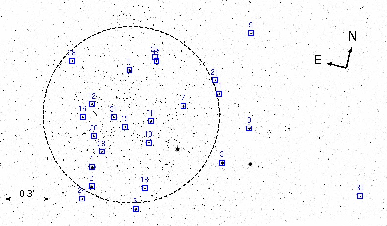
Figure 1: Position of spectroscopic target stars on the sky, overlaid on an archival HST Advanced Camera for Surveys (ACS) image (program 10622, PI: Dolphin). The numbering corresponds to the order of objects as listed in Table 1. The dotted circle marks Pal 4’s half-light radius of $0.6$ arcmin, corresponding to 18 pc at a distance of 102.8 kpc.

2.1 Keck LRIS Photometry

$B$ and $V$ images centered on Pal 4 were obtained with LRIS (Oke et al., 1995) on the night of 1999 January 14. In imaging mode, LRIS has a pixel scale of 0.215 arcsec pixel^-1 and a field of view of $5.8\times 7.3$ arcmin². A series of images were obtained in both $V$ and $B$, with exposure times of $3\times 60$s and $2\times 180$s, respectively. Conditions during the night were photometric, and the FWHM of isolated stars within the frames was measured to be 0$\aas@@fstack{\prime\prime}$65–0$\aas@@fstack{\prime\prime}$75. The images were reduced in a manner identical to that described in Côté et al. (2002) using IRAF. Briefly, the raw frames were bias-subtracted and flat-fielded using sky flats obtained during twilight. Instrumental magnitudes for unresolved objects in the field were derived using the DAOPHOT II software package (Stetson, 1993), and calibrated with observations of several Landolt (1992) standard fields taken throughout the night. The $V$ band magnitudes, which we used to calibrate the cluster’s surface brightness profile (Section 4.1), were found to agree to within 0.02$\pm$0.03 mag with those published by Saha et al. (2005) for stars contained in both catalogs. The final photometric catalog contained 848 objects detected with a minimum point-source signal-to-noise ratio of S/N = 4 in both filters.

2.2 Spectroscopy

On three different nights in February and March 1999, spectra for 24 candidate red giants in the direction of Pal 4 were obtained using HIRES (Vogt et al., 1994) mounted on the Keck I telescope. The targets were selected from the LRIS photometric catalog. The spectra were taken with the C1 decker, which gives a $0\aas@@fstack{\prime\prime}86$ entrance slit and a resolution of $R=45,000$, and cover the wavelength range from 445 to 688 nm. Their position within the cluster is shown in Fig. 1. The exposure times of the spectra were adjusted on a star-to-star basis depending on the individual magnitudes ($17.8<V<19.9{\rm\,mag}$), and varied between 300 and 2400 s with a median value of 1200 s. An observation log and the photometric properties of the target stars are given in Table 1, their coordinates are given in table 1 of Koch & Côté (2010), and their location in the color-magnitude diagram (CMD) can be seen in fig. 1 of the same paper. Based on their location in the CMD, five of the sample stars are probable AGB stars, the remaining 19 stars lie on the RGB.

The spectra were reduced entirely within the IRAF environment, in a manner identical to that described in Côté et al. (2002). The radial velocities of the target stars were obtained by cross-correlating their spectra with those of master templates created from the observations of IAU standard stars, which were taken during the seven observing runs (13 nights) that were devoted to the HIRES survey of globular clusters in the halo. From each cross-correlation function, we measured the heliocentric radial velocity, $v_{r}$, and $R_{\rm TD}$, the Tonry & Davis (1979) estimator of the strength of the cross-correlation peak. Since an important factor in the dynamical analysis of low-mass clusters is an accurate determination of the radial velocity uncertainties, $\epsilon(v_{r})$, 53 repeat measurements for 23 different stars, distributed over different target GCs, were accumulated during the same observing runs. The r.m.s. of the repeat measurements was used to calibrate a relation between $\epsilon(v_{r})$ and $R_{\rm TD}$. Following Vogt et al. (1995), we adopt a relationship of the form $\epsilon(v_{r})={\alpha}/(1+R_{\rm TD})$, where $R_{\rm TD}$ is the Tonry & Davis (1979) estimator of the strength of the cross-correlation peak, and find $\alpha\simeq 9.0$ km s^-1. The resulting radial velocity uncertainties for our Pal 4 target stars range from $0.23$ to $1.31\,{\rm\,km\,s^{-1}}$ (see Table 1).

2.3 HST Photometry

We used archival HST images of Pal 4 obtained with the WFPC2 in GO program 5672 (PI: Hesser, cf. Stetson et al., 1999). The dataset consists of F555W ($V$) and F814W ($I$) band exposures and is the deepest available broad-band imaging of the cluster. The individual exposure times are 8$\times$30 s, 8$\times$60 s and 8$\times\sim 1800$ s in each filter, amounting to total exposure time of $\sim 4.1$ h per filter.

PSF-fitting photometry was obtained using the HSTPHOT package (Dolphin, 2000). In order to refine the image registration, HSTPHOT was first run on the individual images and the resulting catalogs were matched to one of the deep F555W images as a reference using the IRAF tasks xyxymatch and geomap. The derived residual shifts were used for a refined cosmic ray rejection with HSTPHOT’s crmask task, and as an input for the photometry from all images. The latter was obtained by running HSTPHOT simultaneously on all frames with a deep F555W image as the reference or detection image.

To select bona-fide stars from the output catalog, the following quality cuts were applied (for details, see the HSTPHOT user manual): a type parameter of 1 (i.e. a stellar detection), abs(sharpness)$<0.2$, $\chi<2.0$, and in both filters a crowding parameter $<1.5{\rm\,mag}$ and a statistical uncertainty in the magnitude $<0.2{\rm\,mag}$. The resulting CMD, containing 3878 stars, is shown in Fig. 2.

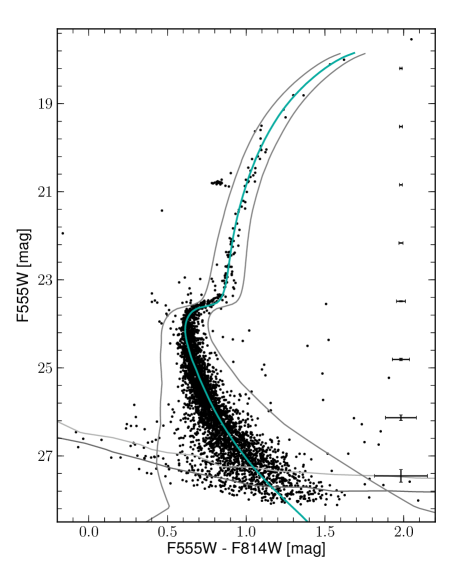
Figure 2: Observed color-magnitude diagram of Pal 4. Errorbars on the right represent the photometric errors derived from artificial star tests. The gray lines at the faint end represent the 80 per cent (light gray) and 50 per cent (dark gray) completeness contours. The isochrone (cyan line) corresponds to an age of 11 Gyr, a metallicity of [Fe/H]=$-1.41$ dex and an $\alpha$-enhancement of [$\alpha$/Fe]=$+0.4$ dex, shifted to the cluster’s distance of $20.06{\rm\,mag}$ at a reddening of $\mathrm{E}(B$-$V)=0.023{\rm\,mag}$. Thin gray curves to the left and to the right of the isochrone represent the color limits used for our analysis of the cluster’s mass function (see Section 4).

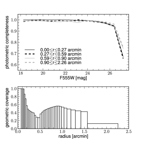
Figure 3: Photometric and geometric completeness of the WFPC2 photometry. Top: The photometric completeness inside the color limits used for our analysis (see Fig. 2) as a function of F555W magnitude derived from the artificial star tests is shown for four radial ranges as denoted in the plot. The radial ranges are defined to contain one fourth of the observed stars each. Bottom: The geometric coverage of the WFPC2 catalog as a function of radius in radial bins containing each one 36th of the observed stars. The fraction represents the area covered by the WFPC2 pointing in a given radial annulus divided by the total area of the annulus.

To assess the photometric uncertainties and completeness of the catalog, HSTPHOT was used to perform artificial star tests with $\sim 275000$ fake stars. We used the program’s option to create artificial stars with distributions similar to the observed stars, both in the CMD, and on the WFPC2 chips, in order to efficiently sample the relevant parameter space. In artificial star mode, the program inserts, star by star, stellar images with given magnitudes and position in all of the frames (using the empirically adjusted PSF for each frame that is constructed during the photometry run) and then performs photometry on this stellar image. It yields as a result a catalog containing the inserted magnitudes and positions, as well as the recovered photometry for each fake star. We applied the same quality cuts to the artificial star catalog as were used to select bona-fide stars in the observed catalog. Photometric uncertainties in a given region of the CMD and on the sky were then estimated from the differences between inserted and recovered magnitudes. The photometric completeness was estimated from the ratio of the number of recovered to the number of inserted artificial stars. The completeness, within the color limits used for our analysis of the cluster’s mass function (see Section 4.3), as a function of F555W magnitude is shown in the top panel of Fig. 3. The different curves correspond to the completeness in different radial ranges, containing each one fourth of the observed stars. At the faint end, the completeness in the inner two annuli drops somewhat faster with decreasing luminosity, which reflects the effect of crowding caused by the higher surface density of stars in the cluster’s center.

The geometric coverage of the WFPC2 photometry was quantified in the following way. For both filters, we ran multidrizzle (Koekemoer et al., 2006) on all frames in that filter, to obtain geometric distortion-corrected combined frames. As a small-scale dither pattern was used in the observations, we then created a coverage mask by selecting all pixels that received, in both filters, at least 25 per cent of the total exposure time. This information can be retrieved from the weight map extension of the drizzled frames. As HSTPHOT uses a single deep exposure as a detection image for the photometry, we additionally required that pixels flagged as covered in the coverage mask were covered also by one of the four chips in that exposure. For this, in order to avoid possible completeness artifacts near chip borders, the chips were assumed to be smaller by 5 pixels on each side. The area covered by the WFPC2 photometry as a function of distance from the cluster’s center was then expressed as the ratio of the area covered by the coverage mask to the total area of a given radial annulus around the cluster’s center. This is shown in the bottom panel of Fig. 3. The stellar positions in the photometric and artificial star catalogs were transformed to the same drizzled coordinate system and to be consistent, stars falling on pixels marked as ‘not covered’ in the coverage mask were rejected. In order to select radial subsamples of stars, we determined the cluster’s center by fitting one-dimensional Gaussians to the distributions of stars projected onto the $x$ and $y$ axes (e.g. Hilker, 2006). As the cluster’s center is close the PC chip’s border in the WFPC2 pointing, for the purpose of determining the center, we performed photometry on more suitable archival data taken with the Wide Field Channel (WFC) of HST’s Advanced Camera for Surveys (ACS) in GO program 10622 (PI: Dolphin, cf. Saha et al., 2011). We used HSTPHOT’s successor DOLPHOT on the program’s F555W (two exposures of 125 s each) and F814W ($2\times 80$ s) exposures to obtain a photometric point source catalog, determined the center form these data and transformed its coordinates to the coordinate system of the WFPC2 catalog.

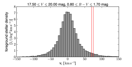
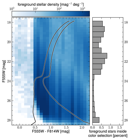
Figure 4: Expected contamination by foreground stars based on the Besançon model. Top: The distribution of foreground stars having magnitudes and colors in the range of our spectroscopic targets as a function of radial velocity. Red vertical lines denote the velocity range of interest. Bottom: The left panel shows the density of foreground stars in the color-magnitude diagram. The black-on-white lines correspond to the region of the CMD used to estimate the mass function of Pal 4 (Section 4.3). Within these color-limits, the fraction of expected foreground stars in the photometric sample, averaged over $0.5$ mag in F555W and shown in the right panel, is below one per cent.

2.4 Foreground contamination

As Pal 4 lies on “our side” of the Galaxy at high Galactic latitude ($l\,\sim$202 deg, $b\,\sim$72 deg), the expected contamination by foreground stars in our spectroscopic and photometric samples is low. To estimate its fraction, we used the Besançon model of the Galaxy (Robin et al., 2003) to obtain a photometric and kinematic synthetic catalog. The model was queried for stars out to 200${\rm\,kpc}$ in the direction of Pal 4. For better number statistics, we used a solid angle of 50 square degrees and the model’s ‘small field’ mode that simulates all stars at the same location and thus ensures that any spatial variation in the foreground that could be present in such a large field is neglected. The remaining model parameters, such as the extinction law and spectral type coverage, were left at their default values.

For a generous estimate of possible foreground contaminants in our spectroscopic sample, we selected from the obtained synthetic catalog stars with magnitudes and colors in the range of the spectroscopic targets (17.5 $\leq V\leq$ 20.0 mag, 0.8 $\leq B-V\leq$ 1.7 mag, cf. Table 1). The top panel of Fig. 4 shows the resulting distribution of stars per square degree as a function of radial velocity. Red vertical lines denote the velocity range of the cluster’s systemic velocity plus and minus three times its velocity dispersion (derived in Section 3). Within this velocity range, $\sim$3 stars per deg² lie inside the color and magnitude range. Scaled to the solid angle covered by the spectroscopic sample (assuming a circular aperture with a radius equal to the largest cluster-centric distance of our sample stars, $\sim 100$ arcsec), this amounts to $\sim 0.01$ stars. It is thus unlikely that the spectroscopic sample contains any foreground stars.

To quantify the expected foreground contamination in the photometric catalog, we transformed the $V$ and $I$ magnitudes of the synthetic foreground stars to F555W and F814W magnitudes, by inverting the Holtzman et al. (1995) WFPC2 to $UBVRI$ transformations. Photometric errors and completeness were then taken into account in the following simple way: for each synthetic foreground star, we selected from our artificial star catalog a random one of the 100 nearest artificial stars in terms of inserted magnitudes (using the euclidean distance in the (F555W, F814W)-plane); if the chosen artificial star was recovered, we added its photometric errors (i.e. recovered minus inserted magnitude) to the magnitudes of the synthetic star; if the artificial star was not recovered, we reject the synthetic foreground star. To take into account the variation of completeness and photometric errors as a function of distance from the cluster center, we assumed the synthetic foreground stars to be homogeneously distributed on the sky and performed the procedure independently on 30 radial sub-samples of the foreground and artificial star catalogs. This results in a foreground catalog that reproduces the photometric errors and completeness limits of our WFPC2 catalog. The density of foreground stars is shown in the bottom left panel of Fig. 4. The two-dimensional histogram was obtained with bins of 0.1 mag in color and 0.25 mag in magnitude and scaled to units of stars per square degree on the sky and square magnitude in the CMD. Selecting stars only in the region of the CMD that was used to derive the mass function of Pal 4 (denoted by the black-on-white lines in the density plot; see Section 4.3) and scaling to the effective area of the WFPC2 field, $\sim 4.76$ arcmin², we calculated that the expected fraction of foreground stars in the photometric sample is below one per cent over the whole luminosity range and therefore negligible. This is shown in the bottom right panel of Fig. 4.

Table 1: Radial velocities for candidate red giants in Pal 4. $(a)$Probable AGB stars based on their location in the CMD.

ID	IDSaha	$R$	$V$	$(B-V)$	$T$	HJD 2,450,000+	$R_{\rm TD}$	$v_{r}$	$\langle v_{r}\rangle$
		(arcsec)	(mag)	(mag)	(s)			(km s-1)	(km s-1)
(1)	(2)	(3)	(4)	(5)	(6)	(7)	(8)	(9)	(10)
Pal4-1	S196	23.3	17.81	1.46	300	11220.9836	18.91	73.59$\pm$0.45	73.33$\pm$0.28
					300	11248.0317	16.50	72.84$\pm$0.52
					300	11221.1684	18.06	73.45$\pm$0.47
Pal4-2	S169	29.9	17.93	1.46	300	11220.9787	16.61	73.95$\pm$0.51	74.42$\pm$0.36
					300	11221.1634	16.31	74.90$\pm$0.52
Pal4-3	S277	41.2	17.82	1.66	300	11221.1388	20.09	72.11$\pm$0.43	72.11$\pm$0.43
Pal4-5	S434	22.9	17.95	1.44	300	11221.1457	17.14	72.24$\pm$0.50	72.41$\pm$0.41
					300	11222.1754	11.36	72.78$\pm$0.73
Pal4-6	S158	34.7	18.22	1.30	420	11220.9647	18.37	72.34$\pm$0.47	72.38$\pm$0.33
					420	11248.0018	10.42	72.47$\pm$0.79
					420	11221.1152	15.36	72.39$\pm$0.55
Pal4-7	S381	23.6	18.55	1.19	600	11221.0986	17.44	73.08$\pm$0.49	72.73$\pm$0.38
					600	11248.0382	14.08	72.21$\pm$0.60
Pal4-8	S364	49.4	18.65	1.17	600	11220.9989	16.59	74.39$\pm$0.51	74.39$\pm$0.51
Pal4-9	S534	63.1	19.00	1.08	750	11221.0124	14.48	71.56$\pm$0.58	71.56$\pm$0.58
Pal4-10	S325	8.9	19.09	1.05	900	11220.9880	16.83	70.11$\pm$0.51	70.68$\pm$0.41
					900	11221.1720	11.86	71.76$\pm$0.70
Pal4-11a	S430	39.2	19.35	0.89	1200	11221.0705	10.12	73.08$\pm$0.81	73.08$\pm$0.81
Pal4-12a	S328	18.1	19.35	0.90	1200	11221.1041	13.09	78.70$\pm$0.64	76.22$\pm$0.43
					1200	11247.9845	14.50	74.19$\pm$0.58
Pal4-15a	S307	2.2	19.38	0.88	1200	11221.0550	9.62	72.33$\pm$0.85	72.33$\pm$0.85
Pal4-16a	S306	19.9	19.43	0.88	1200	11221.0383	13.05	71.09$\pm$0.64	71.09$\pm$0.64
Pal4-17a	S472	28.9	19.45	0.85	1080	11222.0903	11.67	71.87$\pm$0.71	71.87$\pm$0.71
Pal4-18	S186	26.7	19.48	0.98	1200	11221.1275	12.23	71.17$\pm$0.68	71.17$\pm$0.68
Pal4-19	S283	10.4	19.53	0.95	1080	11222.0760	10.41	72.75$\pm$0.79	72.75$\pm$0.79
Pal4-21	S457	40.0	19.64	0.93	1200	11221.0869	9.53	74.41$\pm$0.86	74.41$\pm$0.86
Pal4-23	S235	15.9	19.70	0.93	1500	11222.1575	12.43	73.23$\pm$0.67	73.23$\pm$0.67
Pal4-24	S154	36.0	19.74	0.92	1500	11221.1612	13.50	73.00$\pm$0.62	73.00$\pm$0.62
Pal4-25	S476	29.9	19.77	0.91	1500	11222.1782	9.41	72.84$\pm$0.87	72.84$\pm$0.87
Pal4-26	S265	15.7	19.83	0.91	1500	11222.1389	11.20	72.44$\pm$0.74	72.44$\pm$0.74
Pal4-28	S426	35.9	19.87	0.91	1500	11222.1192	5.89	72.20$\pm$1.31	72.20$\pm$1.31
Pal4-30	S276	99.7	19.89	0.90	1800	11248.0166	9.50	71.33$\pm$0.86	71.33$\pm$0.86
Pal4-31	S315	7.5	19.89	0.93	1500	11222.1982	10.08	72.38$\pm$0.81	72.38$\pm$0.81

3 The systemic velocity and the velocity dispersion

Table 1 summarizes the results of our radial velocity measurements for Pal 4 member stars. Columns (1)–(10) of this table record the names of each program star (second column from identification by Saha et al., 2005), distance from the cluster center, $V$ magnitude, $(B-V)$ color (both from Saha et al., 2005), HIRES exposure time, the heliocentric Julian date of the observation, the Tonry & Davis $R_{\rm TD}$ value, the heliocentric radial velocity, and the error-weighted mean velocity. Six of the stars in our Pal 4 sample were observed twice, and two stars were observed three times. For most stars the difference in radial velocity between the individual measurements is below 1${\rm\,km\,s^{-1}}$. Two stars show a larger discrepancy of 1.65${\rm\,km\,s^{-1}}$ (Pal4-10) and 4.51${\rm\,km\,s^{-1}}$ (Pal4-12, a likely AGB star), potentially due to binarity. For the latter, the two velocity measurements differ by more than $5\sigma$ and the mean of the two measurements stands out in the velocity distribution (see Fig. 5). This suggests that the star should probably be excluded as an outlier. Nevertheless, as its mean velocity is still marginally consistent with the velocity distribution (see below), we will present our kinematical analysis with and without this star (named in the following ‘star 12’).

The mean heliocentric radial velocity and velocity dispersion of Pal 4 were calculated using the maximum likelihood method of Pryor & Meylan (1993). For details about the method see also sec. 3.2 of Baumgardt et al. (2009). Using the 23 clean member stars from Table 1 (i.e. excluding star 12), we obtain a mean cluster velocity of $v_{r}=72.55\pm 0.22{\rm\,km\,s^{-1}}$ and an intrinsic velocity dispersion of $\sigma=0.87\pm 0.18{\rm\,km\,s^{-1}}$. When including star 12, the mean velocity is $v_{r}=72.72\pm 0.27{\rm\,km\,s^{-1}}$ and the velocity dispersion rises to $\sigma=1.15\pm 0.20{\rm\,km\,s^{-1}}$. The cluster’s mean radial velocity is consistent with the determination by Armandroff et al. (1992), $v_{r}=74\pm 1{\rm\,km\,s^{-1}}$.

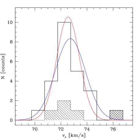
Figure 5: Histogram of radial velocities for all 24 sample stars. The hashed areas correspond to AGB stars, the cross-hashed area corresponds to star 12 at $\sim 76{\rm\,km\,s^{-1}}$. The blue and red curves are the maximum-likelihood Gaussian representations of intrinsic velocity distribution for the total sample of 24 stars and for the sample without star 12, respectively. The sigmas of the Gaussian are the velocity dispersions as derived using the Pryor & Meylan (1993) method.

Figure 6: Radial distribution of stars with velocity measurements in Table 1. The open symbols mark probable AGB stars. The horizontal dotted line marks Pal 4’s error-weighted mean systemic velocity without star 12, and the dashed line the velocity including star 12. The core and half-light radii are indicated by the vertical lines.

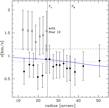
Figure 7: Velocity dispersion profile of Pal 4 using running bins with eight stars in each bin. The black filled symbols denote the velocity dispersion without star 12. The open symbols denote these bins where star 12 was included. The dashed and dotted horizontal lines are the average dispersion values if star 12 is included or excluded, respectively. The vertical lines are the core and half-light radii. Shown as blue solid curve is the dispersion profile expected in Newtonian dynamics for a cluster mass of $2.98\times 10^{4}\rm\,M_{\odot}$ and assuming that mass follows the light of the best-fitting King (1966) model derived in Section 4.1.

Fig. 5 shows the distribution of radial velocities of the 24 cluster members (open histogram). The curves show the maximum-likelihood Gaussian representations of the intrinsic velocity distribution (with and without star 12) using the above values for $v_{r}$ and $\sigma$. As can be seen, the observed radial velocity distribution is well approximated by a Gaussian except for the outlier star 12. For a Gaussian distribution and a sample of 24 stars, one would expect to find a star that is, like star 12, about 3$\sigma$ away from the mean in only 5 per cent of all cases.

In Fig. 6 we show the radial distribution of our measured velocities (star 12 is labeled). The cluster’s mean velocity is marked by the dotted (without star 12) and dashed (with star 12) horizontal line. One third of the 24 sample stars are located at radii equal to or greater than the half-light radius. Thus, the measured velocity dispersion is only slightly biased towards the central value. In this plot no clear trend of a decreasing or increasing velocity dispersion with radius is seen. However, our sampling beyond 50 arcsec radius is very sparse with only two measured velocities. Nevertheless, we derived the line-of-sight velocity dispersion profile with running radial bins, each bin containing eight stars. Fig. 7 shows the resulting velocity dispersion profile. Within a radius of up to 24 arcsec we derived the velocity dispersion either excluding star 12 or including star 12. For the case excluding star 12, we can see a flat velocity dispersion profile that is in good agreement with the expectation from a single-mass, non-mass-segregated King model that is overplotted. When including star 12 one might argue for a declining velocity dispersion profile.

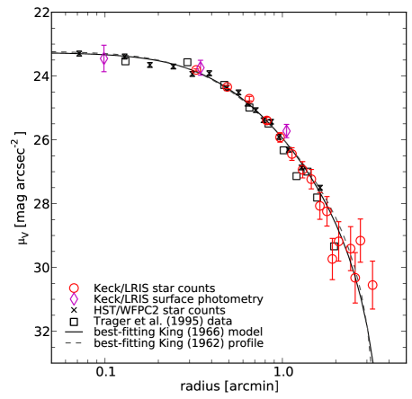
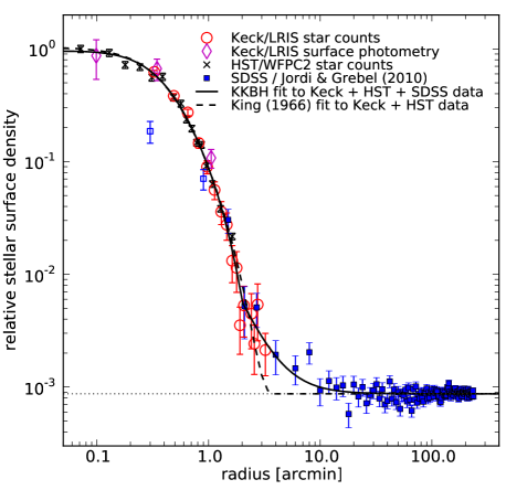
Figure 8: Top: The surface brightness profile of Pal 4. Our LRIS data are represented by filled red circles (derived from star counts) and filled magenta diamonds (from direct surface photometry), the WFPC2 star counts are represented by black crosses. Open squares show the Trager et al. (1995) data based on star counts on photographic plates. The best-fitting King (1966) model to the Keck and HST data is shown as solid curve, the best-fitting King (1962) profile is shown as dashed curve. Bottom: The cluster’s surface density profile (normalized to the innermost point). In order to display the profile on a logarithmic scale we added a virtual background level, indicated as dotted horizontal line. As in the upper panel, red circles and magenta diamonds represent the Keck data and black crosses represent the HST WFPC2 data. Blue squares represent the SDSS-based profile derived by Jordi & Grebel (2010). The two innermost data points of the SDSS-based profile (shown as open squares) were excluded, because they are systematically low due to crowding. The best-fitting KKBH profile to the combined dataset is shown as solid curve. For comparison, the dashed curve represents the best-fitting King (1966) model from the top panel. Pal 4 shows a clearly enhanced stellar density at radii $>3$ arcmin.

Table 2: Structural parameters of Pal 4. A distance of $102.8\pm 2.4$ kpc (Section 4.2) was adopted and all literature values dependent on distance were recalculated using this distance. In calculating the total luminosity L_V, we used a $V$-band extinction of A_V=$3.1\times E(B-V)=0.07$ mag (Section 4.2) and $M_{V,\odot}=4.83$ mag (Binney & Merrifield, 1998).

best-fitting King (1966) model			King (1966) model of
			McLaughlin & van der Marel (2005)
central surface brightness $\mu_{V,0}$	$23.26\pm 0.06$	mag arcsec-2	$23.01^{+0.26}_{-0.22}$	mag arcsec-2
core radius $r_{c}$	$0.43\pm 0.03$	arcmin	$0.33^{+0.05}_{-0.04}$	arcmin
	$13.0\pm 0.8$	pc	$9.8^{+1.4}_{-1.3}$	pc
tidal radius $r_{t}$	$3.90\pm 0.20$	arcmin	$3.30\pm 0.23$	arcmin
	$116.7\pm 6.6$	pc	$98.6\pm 7.2$	pc
concentration $c$	$0.96\pm 0.04$		$0.93\pm 0.1$
2d half-light radius $r_{h}$	$0.62\pm 0.03$	arcmin	$0.51^{+0.03}_{-0.02}$	arcmin
	$18.4\pm 1.1$	pc	$15.3^{+0.9}_{-0.8}$	pc
apparent magnitude $V$	$14.23\pm 0.03$	mag	$14.33^{+0.06}_{-0.03}$	mag
total luminosity LV	$19600\pm 1100$	L⊙	$17900^{+1000}_{-1300}$	L⊙
best-fitting King (1962) profile			King (1962) profile of
			Jordi & Grebel (2010)
central surface brightness $\mu_{V,0}$	$22.96\pm 0.05$	mag arcsec-2	–
core radius $r_{c}$	$0.39\pm 0.02$	arcmin	$0.26\pm 0.10$	arcmin
	$11.7\pm 0.6$	pc	$7.8\pm 3.0$	pc
tidal radius $r_{t}$	$3.46\pm 0.16$	arcmin	$5.30\pm 0.65$	arcmin
	$103.6\pm 5.4$	pc	$158\pm 20$	pc
2d half-light radius $r_{h}$	$0.63\pm 0.03$	arcmin	$0.62\pm 0.24$	arcmin
	$18.8\pm 1.0$	pc	$18.7\pm 7.2$	pc
best-fitting KKBH profile
to combined LRIS, WFPC2 and Jordi & Grebel (2010) data
central surface brightness $\mu_{V,0}$	$22.88\pm 0.17$	mag arcsec-2
inner power-law slope $\gamma$	$-0.04\pm 0.13$
core radius $R_{c}$	$0.44\pm 0.04$	arcmin
	$13.1\pm 0.3$	pc
edge radius $R_{t}$	$2.77\pm 0.12$	arcmin
	$82.9\pm 1.9$	pc
turn-over parameter $\mu$	$0.72\pm 0.05$
outer power-law slope $\eta$	$2.3\pm 0.6$

4 Photometric results

4.1 Surface brightness profile & structural parameters

In the literature there are only few surface brightness profiles and derivations of the structural parameters of Pal 4. As mentioned in the introduction, in a search for extra-tidal features Sohn et al. (2003) used deep wide-field imaging to study the stellar density distribution around Pal 4. Unfortunately, they did not derive a density profile or the cluster’s structural parameters, but adopted the structural parameters from the Harris (1996) catalog. This catalog in its 2003 version quoted the structural parameters derived by Trager et al. (1995) from a compilation of surface photometry. In its updated 2010 version, the Harris (1996) catalog refers to the reanalysis of the Trager et al. (1995) data presented by McLaughlin & van der Marel (2005). Recently, in a search for tidal tails around Galactic GCs, Jordi & Grebel (2010) derived surface density profiles for 17 GCs, including Pal 4. These are based on star counts in the Sloan Digital Sky Survey (SDSS DR7; Abazajian et al., 2009) catalog and the PSF-fitting photometry of SDSS imaging of the inner regions of Galactic GCs by An et al. (2008). However, the authors note that Pal 4 is the most distant GC in their sample and thus the sample includes only stars on the upper RGB. Moreover the cluster’s large distance and the relatively bright limiting magnitude and low spatial resolution of the SDSS make crowding an issue, at least in the cluster’s inner region (r$\la$1 arcmin).

We therefore used our Keck LRIS photometry to measure the structural parameters for Pal 4. The point-source catalog from our LRIS images covers an area of 42.8 arcmin² and contains 777 objects, after excluding stars fainter than $V$ = 24.5 mag to minimize photometric incompleteness. Star counts based on these data were then combined with surface photometry for the innermost regions to construct a composite $V$-band surface brightness profile for the cluster, using the approach described in Fischer et al. (1992). The upper panel of Fig. 8 shows the resulting surface brightness profiles (filled red circles) and additionally three data points from direct surface photometry on the $V$-band image (filled magenta diamonds). As the deeper WFPC2 data sample a much greater number of stars in the cluster’s center, we also included a surface brightness profile derived from star counts in the WFPC2 catalog and the $V$-band magnitudes that HSTPHOT calculates based on the Holtzman et al. (1995) WFPC2 to $UBVRI$ transformations. We included stars down to 27 mag in F555W and corrected the star counts and flux for the radially varying completeness. The resulting profile is shown as black crosses in Fig. 8; due to the inhomogeneous geometric coverage of the WFPC2 catalog, we define radial bins by the requirement that they hold equal numbers of stars. Thus, the Poissonian errorbars on the data points remain constant, while their radial spacing varies.

Both surface brightness profiles agree very well and also show good agreement with the Trager et al. (1995) surface brightness data, which are shown for comparison as open black squares. The figure also shows the best-fitting King (1966, solid curve) model to our LRIS and WFPC2 data, which yields a central surface brightness of $\mu_{V,0}=23.26\pm 0.06$ mag arcsec^-2, a core radius of $r_{c}=0.43\pm 0.03$ arcmin and a tidal radius of $r_{t}=3.90\pm 0.20$ arcmin, corresponding to a concentration of $c=\mathrm{log}(r_{t}/r_{c})=0.96\pm 0.04$ and a (two-dimensional) half-light radius of $r_{h}=0.62\pm 0.03$ arcmin. For comparability, we also fitted a King (1962) profile to our data (dashed curve), which yields core and tidal radii of $r_{c}=0.39\pm 0.02$ and $r_{t}=3.46\pm 0.16$ arcmin and a central surface brightness of $22.96\pm 0.05$ mag arcsec^-2 and reproduces the observations marginally worse in terms of the minimum $\chi^{2}$. Table 2 summarizes our fit results and shows also literature values for comparison. Our best-fitting King (1966) model is somewhat more extended than the one derived by McLaughlin & van der Marel (2005), but otherwise is in good agreement with the latter in terms of central surface brightness, concentration and integrated total luminosity. Comparing our best-fitting King (1962) profile to that of Jordi & Grebel (2010), we find that the latter is more extended and diffuse. This is consistent with the SDSS data underestimating stellar density in the cluster’s center due to crowding as we will see below.

Sohn et al. (2003) noted an excess of stars beyond the cluster’s formal tidal radius, for which they adopted $r_{t}=3.33$ arcmin. As our Keck data reach out to a radius of only $\sim\,3.2$ arcmin, we combine our profile with the SDSS-based profile of Jordi & Grebel (2010). We scaled their background-corrected surface density profile (K. Jordi, private communication) to match the Keck data in the radial range of $1.5-3.2$ arcmin, by interpolating the Keck data to the radii of the SDSS data points and requiring that the median ratio of the two profiles in the overlapping region be one. The merged profile is shown in the lower panel of Fig. 8. As before, diamonds and circles represent the Keck profile, crosses represent the WFPC2 profile. Blue squares represent the SDSS profile. As the SDSS data reach beyond the tidal radius the background-corrected stellar density in individual radial bins can scatter below zero. For the purpose of plotting the profile on a logarithmic scale, we therefore added an artificial background level (shown as dotted horizontal line). The two innermost points of the SDSS data, shown as open squares, deviate from the Keck and WFPC2 profile reflecting the crowding in the SDSS data and we excluded them in our analysis. The dashed line represents the best-fitting King (1966) model from above, and it is obvious that the observed density at large radii falls off less steeply than this model or any other similarly truncated model. We fitted the combined profile with a Küpper et al. (2010, KKBH) template. These templates were designed to fit surface density profiles of GCs out to large cluster radii based on fits to a suite of N-body simulations of Galactic GCs on various orbits. They are a modification of the King (1962) profile including a term for a non-flat core and a term for tidal debris. The best-fitting KKBH profile, shown as solid line in the lower panel of Fig. 8 is found for core and edge radii of $R_{c}=0.44\pm 0.04$ arcmin and $R_{t}=2.77\pm 0.12$ arcmin, a core power-law slope of $\gamma=0\pm 0.1$ and an outer power-law slope of $\eta=2.3\pm 0.6$ that becomes dominant at $\mu R_{t}=2.00\pm 0.15$ arcmin. The shallow slope at large cluster radii may indicate that the cluster is in an orbital phase close to its apogalacticon, although projection effects may play a role in the appearance of the outer part of the density profile. Küpper et al. (2010) find that the surface density profiles of star clusters, as seen in projection onto their orbital planes, are influenced by the tidal debris in this orbital phase: while the slope at large cluster radii, $\eta$, is about 4-5 in most orbital phases, it can reach values of 1-2 in apogalacticon due to orbital compression of the cluster and its tidal tails.

For our following analysis, we will adopt the best-fitting King (1966) model as the cluster’s density profile and come back to the influence of tidal debris in Section 5.2.

4.2 Age determination

To derive the cluster’s age, we determined the isochrone that best reproduces the locus of the principal evolutionary sequences from a subset of isochrones of the Dartmouth Stellar Evolution Database (Dotter et al., 2008). Based on the chemical composition derived by Koch & Côté (2010) from coadded high-resolution spectra of red giants, we adopted [Fe/H]=$-1.41$ dex and an $\alpha$-enhancement of $+0.4$ dex. We determined the best-fitting isochrone using a robust direct fit (similar to Stetson et al., 1999), to the color-magnitude data. As the subgiant branch is almost horizontal in the CMD, even in the F814W vs. F555W-F814W plane (used by Stetson et al. (1999) for that reason), a minimization in one dimension (interpreting the isochrone as ‘color as a function of magnitude’ and comparing the separation in color of each star to the color uncertainty in that magnitude range) runs into problems. Therefore, we employed a $\chi^{2}$ minimization in the (F555W, F814W)-plane, where the uncertainties in both dimensions are uncorrelated, and minimized the squared sum of 2d-distances of each star to the isochrone. To be less sensitive to outliers, instead of $\chi^{2}$, a robust metric that saturates at 5 $\sigma$ was used. Distance and age were varied as free parameters, with the latter ranging from 8 Gyr to 15 Gyr in steps of 0.5 Gyr. We adopted a reddening of $\mathrm{E}(B$-$V)=0.023{\rm\,mag}$ estimated from Galactic dust emission maps and filter-specific extinction to reddening ratios of A${}_{\mathrm{555W}}/\mathrm{E}(B$-$V)$=3.252 and A${}_{\mathrm{F814W}}/\mathrm{E}(B$-$V)$=1.948, taken from table 6 of Schlegel et al. (1998). From this, we obtained a best-fitting age of $11\pm 1$ Gyr and an extinction-corrected distance modulus of $20.06\pm 0.05{\rm\,mag}$. This places the cluster at a distance of $102.8\pm 2.4$ kpc from the Sun. This is slightly closer than the 109.2 kpc derived by Harris (1996, edition 2010) from the mean observed $V$-band magnitude of horizontal branch stars from Stetson et al. (1999), but well within the range of other previous distance determinations of 100 kpc (Burbidge & Sandage, 1958), $105\pm 5$ kpc (Christian & Heasley, 1986) and 104 kpc (VandenBerg, 2000). The age estimate is consistent with Pal 4 being part of the young halo population and $\sim\,1.5$–2 Gyrs younger than ‘classical’, old GCs, as also suggested by the differential analysis relative to M 5 by Stetson et al. (1999) and VandenBerg (2000).

4.3 Mass function

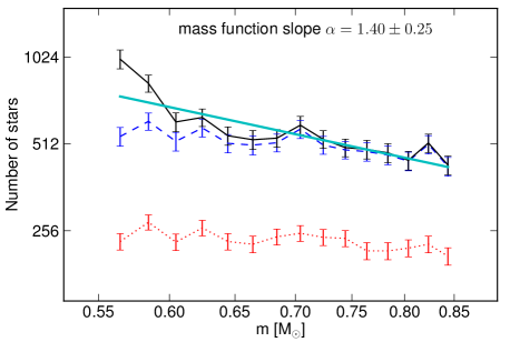
Figure 9: Mass function and power-law fit. The red dotted curve shows the number of observed stars per mass interval, errorbars represent the Poissonian errors on the star counts. The blue dashed curve represents the counts corrected for the missing area coverage, the black solid curve represents the counts additionally corrected for photometric completeness. The cyan line gives the best-fitting power law.

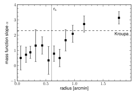
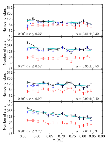
Figure 10: Top: The best-fitting mass function slope $\alpha$ in radial bins containing each one twelfth of the observed stars. Bottom: The mass function in radial bins containing one fourth of the observed stars each. Dotted red curves represent the number of observed stars per mass interval, errorbars represent the Poissonian errors on the star counts. Blue dashed curves are the counts corrected for the missing area coverage in the given radial range. Black solid curves are additionally corrected for photometric completeness. Cyan lines represent the best-fitting power law functions to the completeness-corrected counts. The radial ranges and best-fitting power-law slopes are reported at the bottom of each panel.

We determined the stellar mass function in the cluster in the mass range $0.55\leq\mathrm{M}/\rm\,M_{\odot}\leq 0.85$, corresponding to stars from the tip of the RGB down to the 50 per cent completeness limit in the cluster’s core at the faint end ($17.9{\rm\,mag}\la{\rm F555W}\la 27.6{\rm\,mag}$). We rejected stars that deviated in color from the locus of the isochrone by more than 3$\sigma_{col}$, where $\sigma_{col}$ is the color uncertainty derived from the artificial star results in the corresponding region of the CMD. To avoid rejecting RGB stars, whose scatter around the isochrone is slightly larger than expected purely from photometric uncertainties, we additionally allowed for an intrinsic color spread of $0.02{\rm\,mag}$. This selection removed likely foreground stars, blue stragglers and horizontal branch stars (see Fig. 2). We then assigned to each of the remaining stars a mass based on the isochrone, by interpolating the masses tabulated in the isochrone to the star’s measured F555W magnitude.

At the faint end, crowding affects the photometry and thus the completeness varies slightly with stellar density, or distance from the cluster center. Moreover the geometric coverage of the WFPC2 photometry as a function of radius is very inhomogeneous (see Fig. 3). Therefore, we subdivided our photometric catalog into n radial bins around the cluster center, chosen such that each bin contains one n-th of the observed stars. This is optimal in terms of the Poissonian errors on the star counts, both of the observed stars and of the artificial stars, as the latter were distributed on the sky similarly to the observed stars. The number of radial subdivisions has to be chosen large enough such that completeness and stellar density are approximately constant within each annulus, because otherwise correcting for completeness would bias the results. In practice, we increased the number of bins, n, until the derived mass function slope and cluster mass (Section 4.5) did not vary any more with n. This was the case for n $\geq$ 33 and we chose n $=$ 36 radial bins for the final analysis. In each of these annuli, stars were counted in 12 linearly spaced mass bins (of width $\sim 0.025~{}\rm\,M_{\odot}$). The counts were corrected for the missing area coverage and for photometric completeness in that radial range. Counts from the individual annuli were then summed and fit with a power law of the form $dN/dm\propto m^{-\alpha}$. From this, we obtained a mass function slope of $\alpha=1.4\pm 0.25$ (Fig. 9). This present-day mass function is significantly shallower than a Kroupa (2001) IMF (with $\alpha=2.3$ in this range of masses) and is similar to the mass function in other Galactic GCs (e.g De Marchi et al., 2007; Jordi et al., 2009; Paust et al., 2010).

4.4 Mass segregation

To test for mass segregation, we derived the mass function as a function of radius. As the individual 36 radial annuli contain only $\sim$120 stars each, deriving the mass function in each of them would produce very noisy results. It is thus necessary to bin several of these annuli – after the completeness-corrected counts have been obtained in each annulus individually. As a compromise between signal to noise and radial resolution, we show two different binning schemes: The top panel of Fig. 10 shows the best-fitting mass function slopes derived in radial bins containing each one twelfth of the observed stars. The bottom panel of the same figure shows the mass functions and power-law fits obtained in bins containing each one fourth of the observed stars. It is obvious that the mass function steepens with increasing radius, from $\alpha\la 1$ inside $r\la 1.3\times r_{h}$ to $\alpha\ga$2.3 at the largest observed radii.

4.5 Total mass

In the mass range between $0.55\leq\mathrm{M}/\rm\,M_{\odot}\leq 0.85$, we measure a stellar mass of $5960\pm 110\,\rm\,M_{\odot}$ within the radius covered by the WFPC2 pointing, $r<2.26$ arcmin. We do not correct for the mass contained in blue stragglers and horizontal branch stars that fall outside of our color selection. It is negligible due to their low number ($\sim~{}20$ of each species in our pointing) and we estimate their contribution to be $\la 0.2$ per cent of the total cluster mass.

Assuming the measured mass function slope of $\alpha=1.40\pm 0.25$ to hold down to 0.5 $\rm\,M_{\odot}$ and adopting a Kroupa (2001) mass function, with $\alpha=1.3$, for masses $0.08\leq M/\rm\,M_{\odot}\leq 0.5$, and $\alpha=0.3$ for masses $0.01\leq M/\rm\,M_{\odot}\leq 0.08$, the extrapolated stellar mass in the mass range $0.01\leq\mathrm{M}/\rm\,M_{\odot}\leq 0.85$ is $14500\pm 1300\,\rm\,M_{\odot}$.

To account for the mass contributed by the remnants of higher-mass stars, we assume our observed slope $\alpha$ to hold up to 1.0 $\rm\,M_{\odot}$ and above that a high-mass Kroupa slope of $\alpha=2.3$, and extrapolate the mass function to 60 $\rm\,M_{\odot}$. We follow the prescription of Glatt et al. (2011), assuming stars with initial masses $0.85\leq\mathrm{M}\leq 8\rm\,M_{\odot}$ to have formed 0.6 $\rm\,M_{\odot}$ white dwarfs, and stars with initial masses $8\leq\mathrm{M}\leq 60\rm\,M_{\odot}$ to have formed neutron stars of 1 $\rm\,M_{\odot}$. The extrapolation yields a mass in white dwarfs of $\mathrm{M}_{\mathrm{WD}}$=$8900\pm 800\,\rm\,M_{\odot}$ and a mass in neutron stars of $\mathrm{M}_{\mathrm{NS}}=800\pm 70\,\rm\,M_{\odot}$. In clusters with masses of several times $10^{4}\,\rm\,M_{\odot}$, neutron stars are expected to escape the cluster due to their high initial kick velocities, while virtually all white dwarfs are expected to be retained in the cluster (Kruijssen, 2009). We therefore adopt $\mathrm{M}_{\mathrm{WD}}$=$8900\pm 800\,\rm\,M_{\odot}$ as the mass of stellar remnants.

Based on the best-fitting King (1966) density profile, and approximating that mass follows light, $98.3\pm 0.4$ per cent of the cluster’s mass lies within $r=2.26$ arcmin. Extrapolating out to the tidal radius, the total mass of Pal 4 amounts to $\mathrm{M}_{\mathrm{phot}}=29800\pm 800\,\rm\,M_{\odot}$ including the corrections for low-mass stars and stellar remnants. We note that the uncertainty of the total mass is smaller than the individual uncertainties of the extrapolated high- and low-mass contributions because correlations were fully propagated. These correlations arise from the requirement that the mass function be continuous. As a steeper (shallower) mass function will have more (less) mass in low-mass stars and less (more) mass in high-mass stars and stellar remnants, the uncertainties of the two terms are anti-correlated.

With this mass and the total luminosity derived from the best-fitting King (1966) model, the photometric mass to light ratio of the cluster is M_phot/L${}_{V}=1.52\pm 0.09\,\rm\,M_{\odot}\rm\,L_{\odot}^{-1}$.

To obtain a conservative lower limit on the photometric mass of the cluster, we follow Jordi et al. (2009), assuming the cluster to be significantly depleted in low-mass stars with a declining mass function with $\alpha=-1.0$ for masses $0.01\leq\mathrm{M}/\rm\,M_{\odot}\leq 0.5$. For this hypothetical case, the extrapolation towards lower masses, inclusion of white dwarfs and extrapolation out to the tidal radius yields a total cluster mass of M${}_{\mathrm{decl,phot}}=20100\pm 600\,\rm\,M_{\odot}$.

5 Discussion

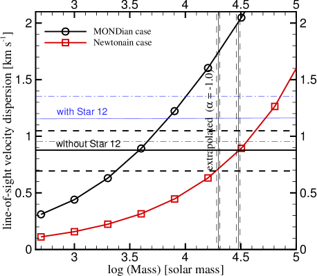
Figure 11: Theoretically predicted line-of-sight velocity dispersion as a function of mass for the Newtonian case (red open squares) and the MONDian case (black open circles). The predictions are taken from recent $N$-body simulations by Haghi et al. (2011). The observed velocity dispersion based on the 23 clean member stars and its uncertainty (Section 3) are shown by black solid and dashed horizontal lines, respectively. Blue solid and dashed lines represent the velocity dispersion and uncertainty obtained when including star 12. For the MONDian case the predicted cluster mass when excluding star 12 and its 1$\sigma$ uncertainty are given by $\mathrm{M}_{\mathrm{MOND}}=3900^{+1400}_{-1500}\,\rm\,M_{\odot}$, while in Newtonian dynamics they are $\mathrm{M}_{\mathrm{Newton}}=32000\pm\,13000\rm\,M_{\odot}$. Including star 12, the predicted masses amount to $\mathrm{M}_{\mathrm{MOND}}=6900^{+3100}_{-2300}\,\rm\,M_{\odot}$ and $\mathrm{M}_{\mathrm{Newton}}=53000^{+18000}_{-16000}\,\rm\,M_{\odot}$ respectively. The vertical black lines indicate the observed total mass (solid line) and its uncertainty (dashed lines), $\mathrm{M}_{\mathrm{phot}}=29800\pm 800\,\rm\,M_{\odot}$, and the mass derived for a mass function significantly depleted in low-mass stars (see text), $\mathrm{M}_{\mathrm{decl,phot}}=20100\pm 600\,\rm\,M_{\odot}$.

5.1 Newtonian and MONDian dynamical mass

In order to see if the observed velocity dispersion and mass of Pal 4 are more compatible with Newtonian or MONDian dynamics, we compare the observed global line-of-sight velocity dispersion with expected velocity dispersions for different cluster masses for the two cases. The expected line-of-sight velocity dispersions of Pal 4 are taken from Haghi et al. (2011), who performed $N$-body simulations of a number of outer halo globular clusters for both Newtonian and MONDian dynamics using the particle-mesh code N-MODY (Londrillo & Nipoti, 2009).

Fig. 11 shows the global line-of-sight velocity dispersion as a function of the cluster mass for the Newtonian (red open squares) and the MONDian case (black open circles). For cluster masses below $10^{5}$ M_⊙, the velocity dispersion in the MONDian case is significantly larger than for the Newtonian case since the acceleration of stars in Pal 4 is below the critical acceleration $a_{0}$ of MOND, making Pal 4 a good test case to discriminate between the two cases. For a line-of-sight velocity dispersion of $0.87\pm 0.18{\rm\,km\,s^{-1}}$ (shown by black horizontal lines in the figure), obtained when excluding the probable outlier star 12 in Section 3, the theoretically predicted mass in MOND is $\mathrm{M}_{\mathrm{MOND}}=3900^{+1400}_{-1500}\,\rm\,M_{\odot}$ and in Newtonian dynamics $\mathrm{M}_{\mathrm{Newton}}=32000\pm\,13000\rm\,M_{\odot}$. This corresponds to mass to light ratios of $\mathrm{M}_{\mathrm{MOND}}/\mathrm{L}_{V}=0.20\pm 0.08\,\rm\,M_{\odot}\,\rm\,L_{\odot}^{-1}$ and $\mathrm{M}_{\mathrm{Newton}}/\mathrm{L}_{V}=1.63\pm 0.67\,\rm\,M_{\odot}\,\rm\,L_{\odot}^{-1}$. For the velocity dispersion including star 12, $\sigma=1.15\pm 0.20{\rm\,km\,s^{-1}}$ (shown by blue horizontal lines in Fig. 11), the theoretically predicted mass in MOND is $\mathrm{M}_{\mathrm{MOND}}=6900^{+3100}_{-2300}\,\rm\,M_{\odot}$ ($\mathrm{M}_{\mathrm{MOND}}/\mathrm{L}_{V}=0.35^{+0.16}_{-0.12}\,\rm\,M_{\odot}\,\rm\,L_{\odot}^{-1}$), while in Newtonian dynamics it is $\mathrm{M}_{\mathrm{Newton}}=53000^{+18000}_{-16000}\,\rm\,M_{\odot}$ ($\mathrm{M}_{\mathrm{Newton}}/\mathrm{L}_{V}=2.70^{+0.93}_{-0.83}\,\rm\,M_{\odot}\,\rm\,L_{\odot}^{-1}$).

In Section 4 we derived a cluster mass of M${}_{\mathrm{phot}}=29800\pm 800\,\rm\,M_{\odot}$ based on the photometry of Pal 4 and assuming a Kroupa IMF for low stellar masses, and a mass of M${}_{\mathrm{decl,phot}}=20100\pm 600\,\rm\,M_{\odot}$ for the case of a declining mass function for low-mass stars. Both values agree well with the expected value for the Newtonian case when excluding star 12. The photometric masses are however significantly larger than the cluster mass derived for the MONDian case. We note, that even if the cluster did not contain any stars less massive than $0.55\,\rm\,M_{\odot}$ (or fainter than our 50 per cent completeness limit of $\la 27.6{\rm\,mag}$ in F555W), its mass of $15100\pm 800\,\rm\,M_{\odot}$ would significantly exceed the MONDian prediction.

The excellent match between photometric and (Newtonian) dynamical masses also means that there is no need to invoke the presence of dark matter in Pal 4, although a small amount of dark matter cannot be excluded. As mentioned in the introduction, Pal 4 is similarly extended and luminous as some of our Galaxy’s ultra-faint dwarf satellites. Its M/L of $\mathrm{M}_{\mathrm{Newton}}/\mathrm{L}_{V}\approx M_{\mathrm{phot}}/\mathrm{L}_{V}\approx 1.6\,\rm\,M_{\odot}\,\rm\,L_{\odot}^{-1}$, however, suggests that it is very different from these dark matter dominated systems and a ‘perfectly normal’ globular cluster. This is also supported by the apparent lack of a metallicity spread in Pal 4, whereas such a spread is detected in most dwarf satellites (see the discussion in Koch & Côté, 2010).

As shown by Gentile et al. (2010), velocity dispersions derived from a small sample of stars suffer from low number statistics. We therefore used Kolmogorov-Smirnov (KS) tests to determine the likelihood of the observed velocity distribution in Newtonian and MONDian dynamics given the photometric cluster mass of $\mathrm{M}_{\mathrm{phot}}=29800\,\rm\,M_{\odot}$ for our sample of radial velocities either including or excluding star 12. Fig. 12 shows the resulting velocity distributions for the Newtonian and MONDian case and the two velocity distributions. In deriving the KS probabilities, we followed Gentile et al. (2010) by not fixing the systemic velocity, but shifting the model distributions in velocity such that the maximum probability was assumed. We note that a KS test in this form is slightly biased to favor MOND, or generally, any model predicting a higher velocity dispersion, because it neglects the broadening of the observed velocity distribution due to the radial velocity uncertainties. However, as the typical velocity uncertainties in our sample are small compared to the cluster’s intrinsic velocity dispersion, the effect is small. For the Newtonian case, a KS test gives a probability of P=0.87 if excluding star 12 and P=0.68 if including star 12. In the MONDian case, the probabilities are P=0.19 and P=0.27 respectively.

Apart from the stochastic effect of the small sample, our velocity dispersion estimate is also subject to the effect of radial sampling. As two thirds of our sample stars are located within the cluster’s half-light radius, the global velocity dispersion will be somewhat lower than our measured value. We do not correct for this effect, but note that it will be small compared to the statistical uncertainty because the cluster’s expected velocity dispersion profile is fairly flat (see Fig. 7). As a lower global velocity dispersion will also lower the predicted masses, the discrepancy between the MONDian prediction and the photometric mass will be larger.

The Newtonian case is therefore favored by the observational data. However, based on the current data alone, MOND cannot be ruled out, so additional radial velocities will be necessary to distinguish between MONDian and Newtonian dynamics. The simulations done by Haghi et al. (2011) indicate that of order 40 radial velocities would be needed for Pal 4 to decrease the MONDian P-values below 0.05 if the internal cluster dynamics is Newtonian. Nevertheless, Pal 4 adds to the growing body of evidence that the dynamics of star clusters in the outer Galactic halo can hardly be explained by MOND, since the velocity dispersions of Pal 4 (this work), Pal 14 (Jordi et al., 2009; Sollima et al., 2012) and NGC 2419 (Baumgardt et al., 2009; Ibata et al., 2011a, b) are consistent with Newtonian dynamics and below the predictions of MOND.

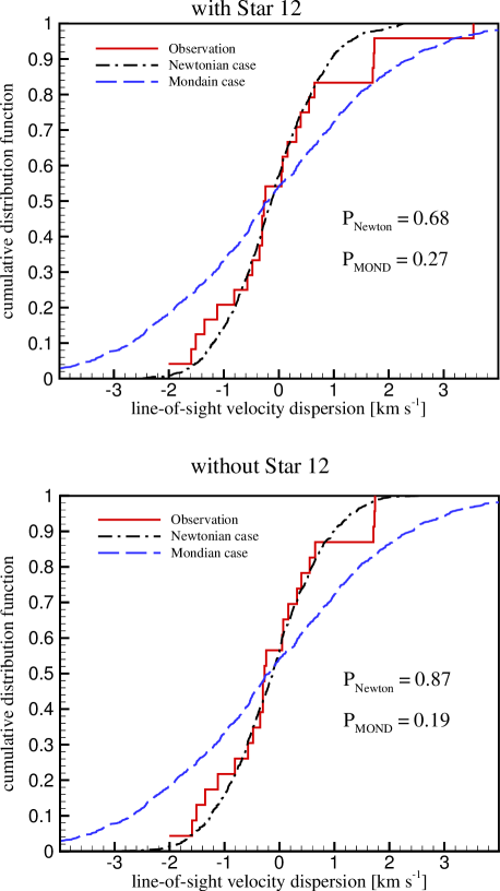
Figure 12: Cumulative distribution function (cdf) of radial velocities for the observed stars (red solid lines) and theoretical distributions assuming Newtonian (black dashed-dotted lines) and MONDian dynamics (blue dashed lines) and a cluster mass of $\mathrm{M}_{\mathrm{phot}}=29800\,\rm\,M_{\odot}$. In the upper panel, star 12 is included, in the lower panel it is excluded. The corresponding probabilities are shown inside the panels.

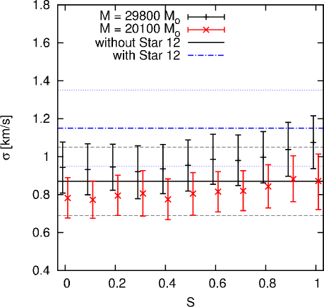
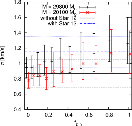
Figure 13: The effect of mass segregation (upper panel) and binarity (lower panel) on the measured velocity dispersions. Error bars show the range (68 per cent) of velocity dispersions of samples of 23 AGB/RGB stars drawn from models of Pal 4. Black solid and dashed horizontal lines represent the observed velocity dispersion and its uncertainty obtained from the 23 clean member stars, blue dash-dotted and dotted lines denote the dispersion and its uncertainty derived including star 12. Upper panel: Mass segregation can bias the measured velocity dispersion by up to 20 per cent since AGB/RGB stars are preferentially located deeper in the cluster potential with increasing degree of mass segregation, $S$. Lower panel: A high binary fraction, $f_{bin}$, can severely affect the measured velocity dispersion. Both effects may imply that Pal 4’s true velocity dispersion is lower than the measured value, in which case the MONDian mass estimate would be more discrepant with the observed mass.

5.2 The effect of mass segregation, unbound stars and binarity

In our analysis we did not take into account the effects of mass segregation, of the presence of unbound stars, and of binaries.

Mass segregation will affect the interpretation of the radial velocity data in three ways: Massive stars, such as the red giant and asymptotic giant branch stars in our kinematic sample will reside more frequently in the cluster’s center, where the gravitational potential is deeper. Therefore they will show a higher velocity dispersion than the global one. On the other hand, energy equipartition will, at a given radius, cause higher mass stars to have lower velocities, lowering the observed velocity dispersion. Moreover, in a mass-segregated cluster, the half-mass radius is larger than the half-light radius. Therefore, when assuming that mass follows light and equating the half-mass radius to the observed half-light radius, a dynamical model will overpredict the velocity dispersion. To quantify these effects, we used the McLuster code (Küpper et al., 2011a) to set up cluster models of Pal 4 with the characteristics obtained in this investigation. We therefore used the best-fitting King (1966) model parameters (see Table 2), a metallicity of [Fe/H]$=-1.41$ dex and a cluster age of 11 Gyr. For the two photometric mass estimates, $\mathrm{M}_{\mathrm{phot}}=29800\,\rm\,M_{\odot}$ and $\mathrm{M}_{\mathrm{decl,phot}}=20100\,\rm\,M_{\odot}$, we generated a total of 126 evolved star clusters containing a number of about 200 RGB and AGB stars each, or 130 respectively in the case of the lower mass estimate. We set up 66 models with a varying degree of mass segregation, $S$. We increase $S$ from zero (unsegregated) to 1.0 (completely segregated) in steps of 0.1, where the observed degree of mass segregation in Pal 4 corresponds approximately to a value of $0.8<S<0.9$, higher values of $S$ are rather unrealistic. Velocity dispersions and their uncertainties were then extracted by repeatedly drawing 23 RGB and AGB stars from the inner 100 arcsec of the cluster models. In a similar approach as Sollima et al. (2012) chose for their analysis Pal 14’s velocity dispersion, we rejected stars that differed by more than $2.5\sigma$ from the mean velocity of each sample to emulate the clipping of likely outliers, such as star 12, in the observations. As shown in the upper panel of Fig. 13, we find that, even in the case of extreme mass segregation, the obtained velocity dispersion rises by not more than 20 per cent compared to the non-segregated case. The velocity dispersion we obtained for Pal 4 may be biased by up to 10 per cent due to mass segregation. However, the error bars in Fig. 13 show only the 68 per cent most likely results. Significantly higher and lower velocity dispersion measurements are still possible with a sample of only 23 stars.

If any of the stars in the radial velocity sample are members of binary systems, the measured velocity dispersion will be increased by the fact that the stars are observed at a random orbital phase of the binaries. This effect can be significant for low-mass stellar systems like Pal 4 (see, e.g., Kouwenhoven & de Grijs, 2008; McConnachie & Côté, 2010; Bradford et al., 2011). The magnitude of this effect depends on the distribution of binary periods and orbital eccentricities and most importantly on the fraction of binaries in the cluster. We studied the effect of binarity by populating 60 further McLuster models of Pal 4 with a varying fraction of binaries, $f_{bin}$. We used the same set-up as for the mass segregation models described above, but added binaries following a Kroupa period distribution and a thermal eccentricity distribution (Kroupa, 1995). Since periods and eccentricities will be subject to internal dynamical evolution on a timescale of 11 Gyr, the binaries were evolved in time with the other stars in the cluster using the binary-star evolution routines by Hurley et al. (2002) that are implemented in McLuster. As for the mass segregated models, velocity dispersions were calculated from random samples of AGB and RGB stars, rejecting velocity outliers. The results are shown in the lower panel of Fig. 13. Just like mass segregation, a high binary fraction can significantly affect the measured velocity dispersion, resulting in a dynamical mass estimate biased towards too high masses.

Finally, unbound stars may contaminate our radial velocity sample. First of all, energetically unbound stars, which have not yet escaped from the cluster (so-called potential escapers) may inflate the velocity dispersion. However, Küpper et al. (2010) showed that potential escapers mainly influence the velocity dispersion profile at large cluster radii. Moreover, also stars within the tidal debris may be misinterpreted as bound cluster members. Küpper et al. (2011b) showed that for clusters in an orbital phase close to apogalacticon the velocity dispersion may be inflated by unbound tidal debris stars, which get pushed close to the cluster due to orbital compression of the cluster and its tidal tails. The shallow slope of Pal 4’s surface density profile at large cluster radii suggests that Pal 4 may be close to its apogalacticon, making such a contamination likely. On the other hand, this effect may be alleviated by the fact that, because of mass segregation, the unbound population will consist preferentially of low-mass stars, while our radial velocity sample consists of more massive red giant and asymptotic giant branch stars.

The combined effects of mass segregation, binaries and unbound stars render it possible that the intrinsic velocity dispersion in Pal 4 is lower than our measured value of $\sigma=0.87\pm 0.18{\rm\,km\,s^{-1}}$. If this was the case, it would further strengthen the case against MONDian dynamics in this cluster, as a decreased velocity dispersion will yield an even lower cluster mass predicted by MOND.

We note that also an anisotropic velocity distribution would affect the velocity dispersion profile of the cluster. While the total kinetic energy is always fixed to one half of the potential energy for a cluster in virial equilibrium, radial anisotropy will increase the velocity dispersion in the cluster’s center compared to the isotropic case and decrease it at large radii, and vice versa for tangential anisotropy. As our radial velocity sample, with 15 stars inside $r_{h}$ and 8 stars outside $r_{h}$, covers a fair range of radii, the effect of anisotropy on our measured dispersion is expected to be only moderate. Correspondingly, Sollima et al. (2012) in their analysis of the similarly distributed radial velocity sample in Pal 14, find that the impact of even purely tangential and or maximally radial anisotropy on the measured velocity dispersion is small.

5.3 Primordial mass segregation

We found clear evidence for mass segregation between main sequence stars in Pal 4. This mass segregation could either have evolved through two-body relaxation and the dynamical friction of high-mass stars or it was already established at the time of the formation of the cluster (e.g. Hillenbrand & Hartmann, 1998). For a half-light radius of 0.6 arcmin, corresponding to 18 pc, and for a cluster mass of $\mathrm{M}=29800\,\rm\,M_{\odot}$, the half-mass relaxation time of Pal 4 is around 14 Gyr, i.e. of the same order as its age. Two-body relaxation is therefore very unlikely as the explanation for the mass segregation in Pal 4: according to the simulations of Gürkan et al. (2004), it takes several half-mass relaxation times until a cluster with a ratio of maximum to average stellar mass of $\mathrm{M}_{\mathrm{max}}/<\mathrm{M}>\approx 4$, which is typical for a globular cluster, goes into core collapse. Unless Pal 4 was significantly more concentrated in the past, the mass segregation in Pal 4 was therefore most likely established by the star formation process itself.

Primordial mass segregation is found in several young Galactic (e.g. Sagar et al., 1988; Hillenbrand, 1997; Hasan & Hasan, 2011) and Magellanic Cloud star clusters (e.g. Fischer et al., 1998; Sirianni et al., 2002). There are also indications for primordial mass segregation in Galactic GCs: Koch et al. (2004) argue that the mass segregation they observed in Pal 5 may be primordial, if the cluster that is currently being disrupted was originally a low-concentration and low-mass cluster. Baumgardt et al. (2008) found that primordial mass segregation together with depletion of low-mass stars by external tidal fields is necessary to explain the present-day mass functions of stars in globular clusters. Pal 14, another diffuse and ‘young halo’ cluster has a flat stellar mass function with slope $\alpha=1.27\pm 0.44$ within the half-light radius (Jordi et al., 2009), which is very similar to the slope that we find for the center of Pal 4. Zonoozi et al. (2011) modeled the evolution of Pal 14 over a Hubble time by direct N-body computations on a star-by-star basis and found that in order to reproduce its observed mass function, either strong primordial mass segregation was necessary, or the initial mass function (IMF) was depleted in low-mass stars. Just like in Pal 4, the half-mass relaxation time of Pal 14 is comparable to its age, and Beccari et al. (2011) found a non-segregated population of blue stragglers in Pal 14, which they interpret as observational support for the fact that dynamical segregation has not affected the cluster yet. If one assumes that Pal 14 formed with a globally normal IMF, its flat central present-day mass function found by Jordi et al. (2009) then suggests that the cluster had primordial mass segregation. This might hold also for Pal 4. According to the simulations of Vesperini et al. (2009) long-lived initially mass-segregated clusters should show a looser structure than initially non-segregated clusters, as the former would lose more mass in the central regions during early stellar evolution. It is therefore an interesting question, if primordial mass segregation is common among diffuse GCs like Pal 4 and Pal 14.

6 Summary

We present a comprehensive analysis of the stellar mass and internal dynamics of Pal 4. Based on a fitting isochrones to a deep CMD and adopting literature values for metallicity, $\alpha$-element enhancement and extinction, we measured the cluster’s age and distance to be $11\pm 1$ Gyr and $102.8\pm 2.4$ kpc respectively. Transforming stellar magnitudes to masses using an isochrone with these parameters, we derived the cluster’s mass function from the tip of the red giant branch down to main sequence stars of $\sim 0.55\,\rm\,M_{\odot}$ in the central $r<2.26$ arcmin. The cluster shows mass segregation, with the mass function steepening from $\alpha\la 1$ inside $r\la 1.3\times r_{h}$ to $\alpha\ga$2.3 outside of $r\ga 1.7\times r_{h}$. As the cluster’s half-mass relaxation time is of the order of the Hubble time, this suggests primordial mass segregation.

Extrapolating the measured mass function towards lower-mass stars and stellar remnants and adopting a Kroupa mass function outside of $0.5<\mathrm{M}<1.0~{}\rm\,M_{\odot}$, as well as extrapolating the mass out to the cluster’s tidal radius based on our surface density profile (Section 4.1), we obtain a total stellar mass of $\mathrm{M}_{\mathrm{phot}}=29800\pm 800\,\rm\,M_{\odot}$.

This is in excellent agreement with the dynamical mass obtained with Newtonian dynamics, $\mathrm{M}_{\mathrm{Newton}}=32000\pm\,13000\rm\,M_{\odot}$, based on the cluster’s observed velocity dispersion of $0.87\pm 0.18{\rm\,km\,s^{-1}}$ derived from radial velocities of 23 clean member stars. The dynamical mass predicted by MOND, $\mathrm{M}_{\mathrm{MOND}}=3900^{+1400}_{-1500}\,\rm\,M_{\odot}$, is significantly below the observed stellar mass. However, in a KS test comparing the observed distribution of radial velocities with that predicted in MONDian dynamics, MOND is also compatible with the data at a probability of $20$ per cent.

Thus the observational data favor Newtonian dynamics, but an extended sample of radial velocities is needed to confidently rule out MOND, if the cluster is governed by Newtonian dynamics.

References

- Abazajian et al. (2009) Abazajian K. N. et al., 2009, ApJS, 182, 543
- An et al. (2008) An D. et al., 2008, ApJS, 179, 326
- Armandroff et al. (1992) Armandroff T. E., Da Costa G. S., Zinn R., 1992, AJ, 104, 164
- Baumgardt et al. (2009) Baumgardt H., Côté P., Hilker M., Rejkuba M., Mieske S., Djorgovski S. G., Stetson P., 2009, MNRAS, 396, 2051
- Baumgardt et al. (2008) Baumgardt H., De Marchi G., Kroupa P., 2008, ApJ, 685, 247
- Baumgardt et al. (2005) Baumgardt H., Grebel E. K., Kroupa P., 2005, MNRAS, 359, L1
- Beccari et al. (2011) Beccari G., Sollima A., Ferraro F. R., Lanzoni B., Bellazzini M., De Marchi G., Valls-Gabaud D., Rood R. T., 2011, ApJ, 737, L3
- Begeman et al. (1991) Begeman K. G., Broeils A. H., Sanders R. H., 1991, MNRAS, 249, 523
- Bekenstein & Milgrom (1984) Bekenstein J., Milgrom M., 1984, ApJ, 286, 7
- Belokurov et al. (2007) Belokurov V. et al., 2007, ApJ, 654, 897
- Binney & Merrifield (1998) Binney J., Merrifield M., 1998, Galactic Astronomy. Princeton Univ. Press, Princeton, NJ
- Bradford et al. (2011) Bradford J. D. et al., 2011, ApJ, 743, 167
- Burbidge & Sandage (1958) Burbidge E. M., Sandage A., 1958, ApJ, 127, 527
- Catelan (2000) Catelan M., 2000, ApJ, 531, 826
- Christian & Heasley (1986) Christian C. A., Heasley J. N., 1986, ApJ, 303, 216
- Côté et al. (2002) Côté P., Djorgovski S. G., Meylan G., Castro S., McCarthy J. K., 2002, ApJ, 574, 783
- Côté et al. (2000) Côté P., Marzke R. O., West M. J., Minniti D., 2000, ApJ, 533, 869
- De Marchi et al. (2007) De Marchi G., Paresce F., Pulone L., 2007, ApJ, 656, L65
- Dolphin (2000) Dolphin A. E., 2000, PASP, 112, 1383
- Dotter et al. (2008) Dotter A., Chaboyer B., Jevremović D., Kostov V., Baron E., Ferguson J. W., 2008, ApJS, 178, 89
- Dotter et al. (2010) Dotter A. et al., 2010, ApJ, 708, 698
- Drukier et al. (1998) Drukier G. A., Slavin S. D., Cohn H. N., Lugger P. M., Berrington R. C., Murphy B. W., Seitzer P. O., 1998, AJ, 115, 708
- Eggen et al. (1962) Eggen O. J., Lynden-Bell D., Sandage A. R., 1962, ApJ, 136, 748
- Fischer et al. (1998) Fischer P., Pryor C., Murray S., Mateo M., Richtler T., 1998, AJ, 115, 592
- Fischer et al. (1992) Fischer P., Welch D. L., Cote P., Mateo M., Madore B. F., 1992, AJ, 103, 857
- Forbes & Bridges (2010) Forbes D. A., Bridges T., 2010, MNRAS, 404, 1203
- Gentile et al. (2010) Gentile G., Famaey B., Angus G., Kroupa P., 2010, A&A, 509, A97
- Glatt et al. (2011) Glatt K. et al., 2011, AJ, 142, 36
- Gürkan et al. (2004) Gürkan M. A., Freitag M., Rasio F. A., 2004, ApJ, 604, 632
- Haghi et al. (2011) Haghi H., Baumgardt H., Kroupa P., 2011, A&A, 527, A33
- Haghi et al. (2009) Haghi H., Baumgardt H., Kroupa P., Grebel E. K., Hilker M., Jordi K., 2009, MNRAS, 395, 1549
- Harris (1996) Harris W. E., 1996, AJ, 112, 1487
- Hasan & Hasan (2011) Hasan P., Hasan S. N., 2011, MNRAS, 413, 2345
- Hilker (2006) Hilker M., 2006, A&A, 448, 171
- Hillenbrand (1997) Hillenbrand L. A., 1997, AJ, 113, 1733
- Hillenbrand & Hartmann (1998) Hillenbrand L. A., Hartmann L. W., 1998, ApJ, 492, 540
- Holtzman et al. (1995) Holtzman J. A., Burrows C. J., Casertano S., Hester J. J., Trauger J. T., Watson A. M., Worthey G., 1995, PASP, 107, 1065
- Hurley et al. (2002) Hurley J. R., Tout C. A., Pols O. R., 2002, MNRAS, 329, 897
- Ibata et al. (2011a) Ibata R., Sollima A., Nipoti C., Bellazzini M., Chapman S. C., Dalessandro E., 2011a, ApJ, 738, 186
- Ibata et al. (2011b) Ibata R., Sollima A., Nipoti C., Bellazzini M., Chapman S. C., Dalessandro E., 2011b, ApJ, 743, 43
- Jordán et al. (2005) Jordán A. et al., 2005, ApJ, 634, 1002
- Jordi & Grebel (2010) Jordi K., Grebel E. K., 2010, A&A, 522, A71
- Jordi et al. (2009) Jordi K. et al., 2009, AJ, 137, 4586
- King (1962) King I., 1962, AJ, 67, 471
- King (1966) King I. R., 1966, AJ, 71, 64
- Koch & Côté (2010) Koch A., Côté P., 2010, A&A, 517, A59
- Koch et al. (2004) Koch A., Grebel E. K., Odenkirchen M., Martínez-Delgado D., Caldwell J. A. R., 2004, AJ, 128, 2274
- Koekemoer et al. (2006) Koekemoer A. M., Fruchter A. S., Hook R. N., Hack W., Hanley C., 2006, in The 2005 HST Calibration Workshop: Hubble After the Transition to Two-Gyro Mode, A. M. Koekemoer, P. Goudfrooij, & L. L. Dressel, ed., p. 423
- Kouwenhoven & de Grijs (2008) Kouwenhoven M. B. N., de Grijs R., 2008, A&A, 480, 103
- Kroupa (1995) Kroupa P., 1995, MNRAS, 277, 1507
- Kroupa (2001) Kroupa P., 2001, MNRAS, 322, 231
- Kruijssen (2009) Kruijssen J. M. D., 2009, A&A, 507, 1409
- Küpper & Kroupa (2010) Küpper A. H. W., Kroupa P., 2010, ApJ, 716, 776
- Küpper et al. (2010) Küpper A. H. W., Kroupa P., Baumgardt H., Heggie D. C., 2010, MNRAS, 407, 2241
- Küpper et al. (2011a) Küpper A. H. W., Maschberger T., Kroupa P., Baumgardt H., 2011a, MNRAS, 417, 2300
- Küpper et al. (2011b) Küpper A. H. W., Mieske S., Kroupa P., 2011b, MNRAS, 413, 863
- Landolt (1992) Landolt A. U., 1992, AJ, 104, 340
- Lane et al. (2010a) Lane R. R., Kiss L. L., Lewis G. F., Ibata R. A., Siebert A., Bedding T. R., Székely P., 2010a, MNRAS, 401, 2521
- Lane et al. (2010b) Lane R. R. et al., 2010b, MNRAS, 406, 2732
- Law & Majewski (2010) Law D. R., Majewski S. R., 2010, ApJ, 718, 1128
- Lee et al. (2007) Lee Y.-W., Gim H. B., Casetti-Dinescu D. I., 2007, ApJ, 661, L49
- Londrillo & Nipoti (2009) Londrillo P., Nipoti C., 2009, Memorie della Societa Astronomica Italiana Supplementi, 13, 89
- Mackey & Gilmore (2004) Mackey A. D., Gilmore G. F., 2004, MNRAS, 355, 504
- Mateo (1996) Mateo M., 1996, in Formation of the Galactic Halo…Inside and Out, H. L. Morrison & A. Sarajedini, ed., Vol. 92, p. 434
- McConnachie & Côté (2010) McConnachie A. W., Côté P., 2010, ApJ, 722, L209