Large Scale Structure in Absorption: Gas within and around Galaxy Voids

Abstract

We investigate the properties of the H i Ly-$\alpha$ absorption systems (Ly-$\alpha$ forest) within and around galaxy voids at $z\lesssim 0.1$. We find a significant excess ($>99$ per cent confidence level, c.l.) of Ly-$\alpha$ systems at the edges of galaxy voids with respect to a random distribution, on $\sim 5$ $h^{-1}$Mpc scales. We find no significant difference in the number of systems inside voids with respect to the random expectation. We report differences between both column density ($N_{\rm HI}$) and Doppler parameter ($b_{\rm HI}$) distributions of Ly-$\alpha$ systems found inside and at the edge of galaxy voids at the $\gtrsim 98$ and $\gtrsim 90$ per cent c.l. respectively. Low density environments (voids) have smaller values for both $N_{\rm HI}$ and $b_{\rm HI}$ than higher density ones (edges of voids). These trends are theoretically expected and also found in gimic, a state-of-the-art hydrodynamical simulation. Our findings are consistent with a scenario of at least three types of Ly-$\alpha$ systems: (1) containing embedded galaxies and so directly correlated with galaxies (referred as ‘halo-like’), (2) correlated with galaxies only because they lie in the same over-dense LSS, and (3) associated with under-dense LSS with a very low auto-correlation amplitude ($\approx$ random) that are not correlated with luminous galaxies. We argue the latter arise in structures still growing linearly from the primordial density fluctuations inside galaxy voids that have not formed galaxies because of their low densities. We estimate that these under-dense LSS absorbers account for $25-30\pm 6$ per cent of the current Ly-$\alpha$ population ($N_{\rm HI}$ $\gtrsim 10^{12.5}$ cm^-2) while the other two types account for the remaining $70-75\pm 12$ per cent. Assuming that only $N_{\rm HI}$ $\geq 10^{14}$ cm^-2 systems have embedded galaxies nearby, we have estimated the contribution of the ‘halo-like’ Ly-$\alpha$ population to be $\approx 12-15\pm 4$ per cent and consequently $\approx 55-60\pm 13$ per cent of the Ly-$\alpha$ systems to be associated with the over-dense LSS.

1 Introduction

The inter-galactic medium (IGM) hosts the main reservoirs of baryons at all epochs (see Prochaska & Tumlinson 2009 for a review). This is supported by both observations (e.g., Fukugita et al., 1998; Fukugita & Peebles, 2004; Shull et al., 2011) and simulations (e.g., Cen & Ostriker, 1999; Theuns et al., 1999; Davé et al., 2010). Efficient feedback mechanisms that expel material from galaxies to the IGM are required to explain the statistical properties of the observed galaxies (e.g., Baugh et al., 2005; Bower et al., 2006; Schaye et al., 2010). Given that galaxies are formed by accreting gas from the IGM, a continuous interplay between the IGM and galaxies is then in place. Consequently, understanding the relationship between the IGM and galaxies is key to understanding galaxy formation and evolution. This has been recognized since the earliest Hubble Space Telescope (HST) spectroscopy of QSOs, where the association between low-$z$ IGM absorption systems and galaxies was investigated for the first time (e.g., Spinrad et al., 1993; Morris et al., 1993; Morris & van den Bergh, 1994; Stocke et al., 1995; Lanzetta et al., 1995).

The large scale environment in which matter resides is also important, as it is predicted (e.g., Borgani et al., 2002; Padilla et al., 2009) and observed (e.g., Lewis et al., 2002; Lopez et al., 2008; Padilla et al., 2010) to have non negligible effects on the gas and galaxy properties. Given that baryonic matter is expected to fall into the considerably deeper gravitational potentials of dark matter, the IGM gas and galaxies are expected to be predominantly found at such locations forming the so called ‘cosmic web’ (Bond et al., 1996). Identification of large scale structures (LSS) like galaxy clusters, filaments or voids and their influence over the IGM and galaxies is then fundamental to a complete picture of the IGM/galaxy connection and its evolution over cosmic time.

With the advent of big galaxy surveys such as the 2dF (Colless et al., 2001) or the Sloan Digital Sky Survey (SDSS, Abazajian et al., 2009) it has been possible to directly observe the nature and extent of the distribution of stellar matter in the local universe. Galaxies tend to lie in the filamentary structure which simulations predict, however, very little is known about the actual gas distribution at low-$z$. In this work we focus on the study of H i Ly-$\alpha$ (hereafter referred simply as Ly-$\alpha$) absorption systems found within and around galaxy voids at $z\lesssim 0.1$.

Galaxy voids are the best candidates to start our statistical study of LSS in absorption. Voids account for up to $60-80\%$ of the volume of the universe at $z=0$ (e.g., Aragón-Calvo et al., 2010; Pan et al., 2012). Some studies have suggested that when a minimum density threshold is reached, voids grow in a spherically symmetric way (e.g., Regos & Geller, 1991; van de Weygaert & van Kampen, 1993). This suggests that voids have a relatively simple geometry, which makes them comparatively easy to define and identify from current galaxy surveys (although see Colberg et al., 2008, for a discussion on different void finder algorithms). Galaxy voids are a unique environment in which to look for evidence of early (or even primordial) enrichment of the IGM (e.g., Stocke et al., 2007). It is interesting that galaxy voids are present even in the distribution of low mass galaxies (e.g., Peebles, 2001; Tikhonov & Klypin, 2009) and so there must be mechanisms that prevent galaxies from forming in such low density environments.

Previous studies of Ly-$\alpha$ absorption systems associated with voids at low-$z$ have relied on a ‘nearest galaxy distance’ (NGD) definition. (e.g., Penton et al., 2002; Stocke et al., 2007; Wakker & Savage, 2009). In order to have a clean definition of void absorbers the NGD must be large, leading to small samples. For instance, Penton et al. (2002) found only 8 void absorbers (from a total of $46$ systems) defined as being located at $>3$ $h^{-1}_{70}$ Mpc from the nearest $\geq L^{*}$ galaxy. Wakker & Savage (2009) found 17 void absorbers (from a total of $102$) based on the same definition. Stocke et al. (2007) had to relax the previous limit to $>1.4$ $h^{-1}_{70}$ Mpc in order to find $61$ void absorbers (from a total of $651$ systems), although only 12 were used in their study on void metallicities. Note that a low NGD limit (of $1.4$ $h^{-1}_{70}$ Mpc) could introduce some contamination of not-void absorbers. This is because filaments in the ‘cosmic web’ are expected to be a couple of Mpc in radius (González & Padilla, 2010; Aragón-Calvo et al., 2010; Bond et al., 2010). Considering the Local Group as an example, being $1.4$ $h^{-1}_{70}$ Mpc away from either the Milky Way or Andromeda cannot be considered as being in a galaxy void. On the other hand, given that there is a population of galaxies inside voids (e.g., Rojas et al., 2005; Park et al., 2007; Kreckel et al., 2011), the NGD definition could also miss some ‘real’ void absorbers relatively close to bright isolated galaxies. In fact, Wakker & Savage (2009) found that there may be no void absorbers in their sample (based on the NGD definition) if the luminosity limit to the closest galaxy is reduced to $0.1L^{*}$. Note however that their sample is very local ($z\leq 0.017$ or $\lesssim 70$ $h^{-1}_{70}$ Mpc away), and it might be biased because of the local overdensity to which our Local Group belongs.

In this work we use a different approach to define void absorption systems. We based our definition on current galaxy void catalogs (typical radius of $>14$ $h^{-1}_{70}$ Mpc), defining void absorbers as those located inside such galaxy voids. This leads to larger samples of well identified void absorbers compared to previous studies. Moreover, this approach allows us to define a sample of absorbers located at the very edges of voids, that can be associated with walls, filaments and nodes, allowing us to get some insights in the distribution of gas in the ‘cosmic web’ itself. This definition is different from the NGD based ones and it focuses on the ‘large scale’ ($\gtrsim 10$ Mpc) relationship between Ly-$\alpha$ forest systems and galaxies. The results from this work will offer a good complement to previous studies based on ‘local’ scales ($\lesssim 2$ Mpc).

Our paper is structured as follows. The catalogs of both Ly-$\alpha$ systems and galaxy voids that we used in this work are described in §2. Definition of our LSS in absorption samples and the observational results are presented in §3. We compare our observational results with a recent cosmological hydrodynamical simulation in §4. We discuss our findings in §5 and summarize them in §6. A check for systematic effects and biases that could be present in our data analysis is presented in Appendix A. All distances are in co-moving coordinates assuming $H_{0}=100\ h$ km s^-1Mpc^-1, $h=0.71$, $\Omega_{\rm m}=0.27$, $\Omega_{\rm\Lambda}=0.73$, $k=0$ cosmology unless otherwise stated. This cosmology was chosen to match the one adopted by Pan et al. (2012) (D. Pann, private communication; see §2.2).

2 Data

2.1 Gas in absorption

We use QSO absorption line data from the Danforth & Shull (2008, hereafter DS08) catalog, which is the largest high-resolution ($R\equiv\frac{\Delta\lambda}{\lambda}\approx 30\,000-100\,000$), low-$z$ IGM sample to date. Briefly, the catalog lists 651 Ly-$\alpha$ absorption systems at $z_{\rm abs}\leq 0.4$, with associated metal lines (O vi, N v, C iv, C iii, Si iv, Si iii and Fe iii; when the spectral coverage and signal-to-noise allowed their observation), taken from 28 AGN observed with both the Space Telescope Imaging Spectrograph (STIS, Woodgate et al., 1998) on the HST, and the Far Ultraviolet Spectroscopic Explorer (FUSE, Moos et al., 2000). The systems are characterized by their rest-frame equivalent widths ($W_{r}$), or upper limits on $W_{r}$, for each individual transition. Column densities ($N_{\rm HI}$) and Doppler parameters ($b_{\rm HI}$) were inferred using the apparent optical depth method (AODM, Savage & Sembach, 1991) and/or Voigt profile line fitting. In particular for the Ly-$\alpha$ transition, a curve-of-growth (COG) solution was used when other Lyman series lines were available (see also Appendix A.2). We refer the reader to DS08 (and references therein) for further description and discussion.

In order to identify absorbing gas associated with LSS (drawn from the SDSS DR7), we use a subsample of the DS08 AGN sightlines that intersect the SDSS volume (PG 0953$+$414, Ton 28, PG 1116$+$215, PG 1211$+$143, PG 1216$+$069, 3C 273, Q 1230$+$0115, PG 1259$+$593, NGC 5548, Mrk 1383 and PG 1444$+$407; see Table 1). Despite the fact that PG 1216$+$069 spectrum has a poor quality, it is still possible to find strong systems in it, and so we decided to do not exclude it from the sample (this inclusion does not affect our results; see §3.1). We use the rest of the sightlines in the DS08 catalog to derive the general properties of the average absorber for comparison (see Appendix A.1).

Table 1: IGM sightlines from DS08 that intersect the SDSS survey.

Sight Line	RA (J2000)	Dec (J2000)	$z_{\rm AGN}$	$S/N$
PG 0953$+$414	09 56 52.4	$+$41 15 22	0.23410	$14$
Ton 28	10 04 02.5	$+$28 55 35	0.32970	$9$
PG 1116$+$215	11 19 08.6	$+$21 19 18	0.17650	$18$
PG 1211$+$143	12 14 17.7	$+$14 03 13	0.08090	$30$
PG 1216$+$069	12 19 20.9	$+$06 38 38	0.33130	$3$
3C 273	12 29 06.7	$+$02 03 09	0.15834	$35$
Q 1230$+$0115	12 30 50.0	$+$01 15 23	0.11700	$12$
PG 1259$+$593	13 01 12.9	$+$59 02 07	0.47780	$12$
NGC 5548	14 17 59.5	$+$25 08 12	0.01718	$13$
Mrk 1383	14 29 06.6	$+$01 17 06	0.08647	$16$
PG 1444$+$407	14 46 45.9	$+$40 35 06	0.26730	$10$

In our analysis we focus on statistical comparisons of the H i properties in different LSS environments. Metal systems have smaller redshift coverage and lower number densities than Ly-$\alpha$ absorbers. Consequently, we do not aim to draw statistical conclusions from them. We intend to pursue metallicity studies in future work.

2.2 Galaxy voids

We use a recently released galaxy-void catalog from SDSS DR7 galaxies (Pan et al., 2012, hereafter P12), which is the largest galaxy-void sample to date. Hereafter we will use the term void to mean galaxy-void unless otherwise stated. P12 identified $\gtrsim 1000$ cosmic voids using the VoidFinder algorithm described by Hoyle & Vogeley (2002), with redshifts between $0.01\lesssim z\lesssim 0.102$. To summarize, it first uses a nearest neighbor algorithm on a volume limited galaxy survey. Galaxies whose third nearest neighbor distance is greater than $6.3$ $h^{-1}$Mpc are classified as potential void galaxies, whereas the rest are classified as wall galaxies. Void regions are identified by looking for maximal empty spheres embedded in the wall galaxy sample. These individual void spheres have radii between $10<R_{\rm void}\lesssim 25$ $h^{-1}$Mpc, with mean radius $\langle R_{\rm void}\rangle\approx 13$ $h^{-1}$Mpc. The minimum radius of $10$ $h^{-1}$Mpc for the void spheres was imposed. Only galaxies with spectroscopic redshifts were used and therefore we expect the uncertainties in the void centers and radii to be small ($\lesssim 1$ Mpc; we will discuss the effects of peculiar velocities in §3.1). Independent void regions are defined by combining all the adjacent spheres that share more than $10\%$ of their volume with another. Void galaxies are defined as those galaxies that lie within a void region. We refer the reader to P12 for further description and discussion.

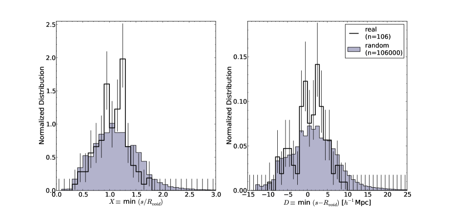
Figure 1: Normalized (in area) distribution of H i absorption systems as a function of $X$ (left panel; $0.1$ binning) and $D$ (right panel; $1$ $h^{-1}$Mpc binning) for both real and random samples. Error bars correspond to the Poissonian uncertainty from the analytical approximation $\sigma^{+}_{n}\approx\sqrt{n+\frac{3}{4}}+1$ and $\sigma^{-}_{n}\approx\sqrt{n-\frac{1}{4}}$ (Gehrels, 1986). Real and random distributions are different at a $\gtrsim 99.5\%$ confidence level (see §3.1 for further details).

In our analysis, for simplicity, we use the individual spheres as separate voids instead of using the different independent void regions. This choice has the following advantages. First, it allows us to use a perfectly spherical geometry, making it possible to characterize each void by just one number: its radius. Thus, we can straightforwardly scale voids with different sizes for comparison. Secondly, this approach allows us to identify regions at the very edges of the voids. P12 found that the number density of galaxies has a sharp peak at a distance $\approx R_{\rm{void}}$ from the center of the void spheres, a clear signature that walls are well defined (at least from the point of view of bright galaxies at low redshifts). This is also consistent with the predictions of linear gravitation theory (e.g., Icke, 1984; Sheth & van de Weygaert, 2004) and dark matter simulations (e.g., Benson et al., 2003; Colberg et al., 2005; Ceccarelli et al., 2006, P12). Therefore, by looking for absorption systems very close to the edge of voids, we expect to trace a different cosmic environment. Thirdly, using the individual void spheres securely identifies void regions. The void-edge sample on the other hand, could be contaminated by void regions associated with the intersections of two void spheres. We checked that this is not the case though (see §3.2). This contamination should only reduce any possible difference between the two samples rather than enhance them. We also note that systematic uncertainties produced by assuming voids to be perfect spheres should also act to reduce any detected difference.

3 Data analysis and results

3.1 Number density of absorption systems around voids

We have cross-matched the IGM absorption line catalog from DS08 (see §2.1) with the void catalog from P12 (see §2.2). A total of $106$ Ly-$\alpha$ absorption systems were found in the $11$ sightlines that intersect the void sample volume (i.e., those with $0.01\leq z_{\rm abs}\leq 0.102$).

We first look for a possible difference in the number density of Ly-$\alpha$ systems as a function of the distance to voids. We take two approaches. First, we define $X$ as the three-dimensional distance between an absorption system and the closest void center in $R_{\rm{void}}$ units, so

$$X\equiv\min_{\rm{sample}}\frac{s}{R_{\rm{void}}}\ \rm{,}$$ (1)

where $s$ is the co-moving distance between the center of the closest void and the absorber. Thus, $0\leq X<1$ corresponds to absorption systems inside voids and $X>1$ corresponds to absorption systems outside voids. A value of $X\approx 1$ corresponds to absorption systems around void edges as defined by the galaxy distribution.

The second approach defines $D$ as the three-dimensional distance between an absorption system and the closest void edge in co-moving $h^{-1}$Mpc, so

$$D\equiv\min_{\rm{sample}}(s-R_{\rm{void}})\ [h^{-1}\rm{Mpc].}$$ (2)

Negative $D$ values correspond to absorption systems inside voids while positive values correspond to absorbers outside voids. Values of $D\approx 0$ $h^{-1}$Mpc are associated with absorption systems around void edges as defined by the galaxy distribution.

Distances were calculated assuming the absorption systems to have no peculiar velocities with respect to the center of the voids. Although this assumption might be realistic for gas inside voids, it might not be the case for gas residing in denser environments, where gas outflows from galaxies might dominate. However, some studies have suggested that the bulk of Ly-$\alpha$ forest lines have little velocity offset with respect to galaxies (e.g., Theuns et al., 2002; Wilman et al., 2007). As an example, a velocity difference of $\sim 200$ km s^-1 at redshift $z_{\rm abs}\lesssim 0.1$ would give an apparent distance shift of the order of $\sim 2$ $h^{-1}$Mpc, which is somewhat higher than, but comparable to the systematic error of the void center determination (given that voids regions are not perfectly spherical as assumed here). Note that the uncertainty in the void center is smaller than the uncertainty of a single galaxy because the void is defined by an average over many galaxies. As previously mentioned, such an uncertainty should not artificially create a false signal but rather should dilute any real difference.

Although the $X$ and $D$ coordinates are not independent, we decided to show our results using both. This has the advantage of testing the consistency of our results using two slightly differently motivated definitions. $X$ is a scaled coordinate, good for stacking voids of different radius. It is also good for comparisons with some of the P12 results. $D$ gives a direct measure of the actual distances involved, while still using $R_{\rm void}$. For convenience, results associated with the $X$ definition will be shown normally in the text while results associated with the $D$ definition will be shown in parenthesis: $X$ ($D$) format.

Figure 1 shows the histogram of absorption systems as a function of $X$ and $D$ (left and right panel respectively). In order to show the effects of the geometry of the survey, the random expectations are also shown (shaded distributions). To generate the random samples, we placed $1000$ random absorption systems per real one, uniformly between $z_{\rm lim}<z_{\rm abs}\leq 0.102$ for each sightline, where $z_{\rm lim}$ corresponds to the maximum of $0.01$ and the minimum observed redshift for a Ly-$\alpha$ in that sightline. In this calculation we have masked out spectral regions over a velocity window of $\pm 200$ km s^-1 around the position where strong Galactic absorption could have been detected (namely: C i, C ii, N v, O i, Si ii, P iii, S i, S ii, Fe ii and Ni ii) before the random redshifts are assigned. A total of $106\,000$ random absorbers were generated. We observe a relative excess of absorption systems compared to the random expectation between $X\simeq 0.9$–$1.3$ and/or $D\simeq-2$–$4$ $h^{-1}$Mpc. Assuming Poisson uncertainty, there were $61\pm 8$ ($65\pm 8$) observed, while $\approx 38.3\pm 0.2$ ($42.4\pm 0.2$) were expected from the random distribution. This corresponds to an $\approx 3\sigma$ excess. Similarly, there is a significant ($\approx 3\sigma$) deficit of absorption systems at $X\gtrsim 1.3$ and/or $D\gtrsim 4$ $h^{-1}$Mpc, for which $17\pm 4$ ($19\pm 4$) systems were observed compared to the $33.9\pm 0.2$ ($34.1\pm 0.2$) randomly expected. We also checked that such an excess and deficit did not appear by chance in $1000$ realizations, consistent with the $<0.1\%$ probability of occurrence. No significant difference is found for systems at $X\lesssim 0.9$ and/or $D\lesssim-2$ $h^{-1}$Mpc, for which the $28\pm 5$ ($22\pm 5$) found are consistent with the random expectation of $33.4\pm 0.2$ ($29.0\pm 0.2$). The Kolmogorov-Smirnov (KS) test between the full unbinned samples gives a $\approx 0.3\%$ ($0.5\%$) probability that both the random and the real data come from the same parent distribution. We checked that no single sightline dominates the signal by removing each individual one and repeating the previous calculation. We also checked that masking out the spectral regions associated to possible Galactic absorption does not have an impact on our results as the same numbers (within the errors) are recovered when these regions are not excluded. These results hint at a well defined gas structure around voids, possibly analogous to that seen in galaxies. The current data are not sufficient to confirm (at a high confidence level) the reality of the apparent two-peaked shape seen in the real distributions however.

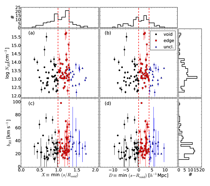
Figure 2: Panels (a) and (b) show the distribution of column densities of H i as a function of $X$ and $D$ respectively. Panels (c) and (d) show the distribution of Doppler parameters as a function of $X$ and $D$ respectively. Our LSS samples are shown by different color/symbols: void (black circles), void-edge (red squares) and unclassified (blue triangles). Histograms are also shown around the main panels. Vertical red dashed lines show the limits of our LSS definitions (see §3.2).

Table 2: General properties of our LSS samples.

Sample	$\log(N_{HI}[\rm{cm}^{-2}])$		$b_{HI}$ [km s-1]
	mean	median	mean	median
Void	13.21 $\pm$ 0.67 (13.21 $\pm$ 0.67)	13.05 (13.05)	28 $\pm$ 15 (28 $\pm$ 15)	25 (25)
Edge	13.50 $\pm$ 0.70 (13.52 $\pm$ 0.69)	13.38 (13.38)	33 $\pm$ 17 (34 $\pm$ 17)	28 (28)
Unclassified	13.20 $\pm$ 0.45 (13.17 $\pm$ 0.48)	13.36 (13.36)	33 $\pm$ 11 (31 $\pm$ 11)	32 (31)

3.2 Definition of large scale structure in absorption

We define three LSS samples observed in absorption:

• Void absorbers: those absorption systems with $X<1$ and/or $D<0$ $h^{-1}$Mpc. A total of $45$ ($45$) void absorbers were found.

• Void-edge absorbers: those absorption systems with $1\leq X<1.3$ and/or $0\leq D<4$ $h^{-1}$Mpc. A total of $44$ ($42$) void-edge absorbers were found.

• Unclassified absorbers: those absorption systems with $X\geq 1.3$ and/or $D\geq 4$ $h^{-1}$Mpc. A total of $17$ ($19$) unclassified absorbers were found.

To be consistent with the galaxy-void definition, we use $X=1$ and/or $D=0$ $h^{-1}$Mpc as the limits between void and void-edge absorbers. The division between void-edge and unclassified absorbers was chosen to match the transition between the overdensity to underdensity of observed absorbers compared to the random expectation at $X>1$ and/or $D>0$ $h^{-1}$Mpc (see Figure 1).

We have assumed here that the center of galaxy voids will roughly correspond to the center of gas voids, however that does not necessarily imply that gas voids and galaxy voids have the same geometry. In fact, as we do not find a significant underdensity in the number of void absorbers with respect to the random expectation, it is not clear that such voids are actually present within the Ly-$\alpha$ forest population. Of course, the fact that we do not detect this under-density, does not imply that the gas voids are not there. A better way to look at these definitions is by considering void absorbers as those found in galaxy under-densities (galaxy voids) and void-edge absorbers as those found in regions with a typical density of galaxies. We do not have a clear picture of what the unclassified absorbers correspond to. Unclassified absorbers are those lying at the largest distances from the cataloged voids, but this does not necessarily imply that they are associated with the highest density environments only. In fact, there could be high density regions also located close to void-edges, at the intersection of the cosmic web filaments. Given that voids of radius $\lesssim 10$ $h^{-1}$Mpc are not present in the current catalog it is also likely that some of the unclassified absorbers are associated with low density environments. Therefore, one interpretation of unclassified-absorbers could be as being a mixture of all kind of environments, including voids, void-edges and high density regions.

We checked the robustness of these definitions by looking at the number of voids and void-edges which can be associated with a given absorber. In other words, for a given absorption system, we counted how many voids or void-edges could have been associated with it by taking simply $X\equiv s/R_{\rm void}$ or $D\equiv s-R_{\rm void}$ (in contrast to having taken the minimum values). Out of the $45$ void absorbers, $41$ are associated with only one void and $4$ are associated with $2$ voids, independently of the definition used (either $X$ or $D$). Likewise, out of the $44$ ($42$) void-edge absorbers, $31$ ($28$) are associated with just one void-edge, $12$ ($13$) are associated with two void-edges and $1$ ($1$) is associated with three void-edges. This last system is located at $X=1.04$ ($D=0.55$ $h^{-1}$Mpc) and has $N_{\rm HI}$ $=10^{14.17\pm 0.35}$ cm^-2 and $b_{\rm HI}$ $=25^{+21}_{-7}$ km s^-1 at a redshift of $z_{\rm abs}=0.01533$. From these values the system does not seem to be particularly peculiar. Finding an association with more than two void-edges is not surprising as long as the filling factor of voids is not small. Void absorbers have on average $1.1\pm 0.3$ voids associated with them, with a median of $1$. Void-edge absorbers have in average $1.3\pm 0.5$ ($1.4\pm 0.5$) void-edges associated with them, with a median of $1$($1$). These values give a median one-to-one association. Therefore, we conclude then that the LSS definitions used here are robust.

3.3 Properties of absorption systems in different large scale structure regions

Figure 2 shows the distribution of column densities and Doppler parameters as a function of both $X$ and $D$. At first sight, no correlation is seen between $N_{\rm HI}$ or $b_{\rm HI}$ and distance to the center of voids. Table 2 gives the mean and median values of $\log(N_{HI}[\rm{cm}^{-2}])$ and $b_{\rm HI}$  for our void, void-edge and unclassified absorption systems. These results show consistency within $1\sigma$ between the three LSS samples.

Table 3: Kolmogorov-Smirnov (KS) test probabilities between different samples.

	void/edge	void/uncl.	edge/uncl.	void/not-void	edge/not-edge	uncl./not-uncl.
KS-Prob($\log N_{\rm HI}$)	2% (0.7%)	74% (66%)	56% (24%)	4% (4%)	3% (0.6%)	64% (54%)
KS-Prob($b_{\rm HI}$)	8% (6%)	18% (17%)	71% (75%)	7% (7%)	20% (14%)	32% (32%)

A closer look at the problem can be taken by investigating the possible differences in the full $N_{\rm HI}$ and $b_{\rm HI}$ distributions of void, void-edge and unclassified absorbers.

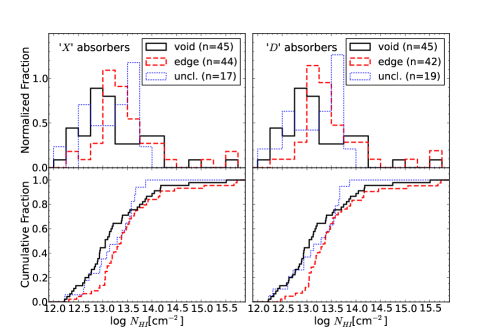
Figure 3: H i column density distribution for the three different LSS defined in this work (see §3.2): void absorbers (solid-black lines), void-edge absorbers (red-dashed lines) and unclassified absorbers (blue-dotted lines). Top panels show the normalized distribution using arbitrary binning of $0.5$ dex. Bottom panels show the cumulative distributions for the unbinned samples. Left and right panels correspond to absorbers defined using $X$ and $D$ coordinates respectively.

3.3.1 Column density distributions

Figure 3 shows the distribution of column density for the three different LSS defined above (see §3.2). The top panels show the normalized fraction of systems as a function of $N_{\rm HI}$ (arbitrary binning), whilst the bottom panels show the cumulative distributions (unbinned). We see from the top panels that this distribution seems to peak systematically at higher $N_{\rm HI}$ from void to void-edge and from void-edge to unclassified absorbers. We also observe a suggestion of a relative excess of weak systems ($N_{\rm HI}\lesssim 10^{13}$ cm^-2) in voids compared to those found in void-edges. This can also be seen directly in Figure 2 (see panels (a) and (b)). The KS test gives a probability $P^{\log N}_{\rm void/edge}\approx 2\%$ ($0.7\%$) that void and void-edge absorbers come from the same parent distribution. This implies a $>2\sigma$ difference between these samples. No significant difference is found between voids or void-edges with unclassified absorbers, for which the KS test gives probabilities of $P^{\log N}_{\rm void/uncl.}\approx 74\%$ ($66\%$) and $P^{\log N}_{\rm edge/uncl.}\approx 56\%$ ($24\%$) respectively. These results can be understood by looking at the bottom panels of Figure 3, as we see that the maximum difference between the void and void-edge absorbers distributions is at $N_{\rm HI}\lesssim 10^{13.8}$ cm^-2. On the other hand, no big differences are observed at $N_{\rm HI}\gtrsim 10^{13.8}$ cm^-2. In fact, by considering just the systems at $N_{\rm HI}<10^{13.8}$ cm^-2, the significance of the difference between void and void-edge absorbers is increased, with $P^{\log N}_{\rm void/edge}\approx 0.9\%$ ($0.2\%$). Likewise, at $N_{\rm HI}\geq 10^{13.8}$ cm^-2, void and void-edge absorber distributions agree at the $\approx 86\%$ ($86\%$) confidence level. We note however that there were $\leq 10$ systems per sample for this last comparison and therefore, it is likely to be strongly affected by low number statistics.

We also investigated possible differences between void, void-edge and unclassified absorbers and their complements (i.e., all the systems that were not classified as these: not-void, not-void-edge, not-unclassified). Not-voids correspond to the combination of void-edge and unclassified absorbers and so on. The KS gives probabilities of $P^{\log N}_{\rm void/not-void}\approx 4\%$ ($4\%$), $P^{\log N}_{\rm edge/not-edge}\approx 3\%$ ($0.6\%$) implying that void and void-edge absorbers are somewhat inconsistent with their complements. On the other hand, the distribution of unclassified absorbers is consistent with the distribution of their complements with a KS probability of $P^{\log N}_{\rm uncl./not-uncl.}\approx 64\%$ ($54\%$). These results are summarized in Table 3.

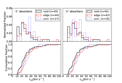
Figure 4: H i Doppler parameter distribution for the three different LSS defined in this work (see §3.2): void absorbers (black-solid lines), void-edge absorbers (red-dashed lines) and unclassified absorbers (blue-dotted lines). Top panels show the normalized distribution using arbitrary binning of $5$ km s^-1. Bottom panels show the cumulative distributions for the unbinned samples. Left and right panels correspond to absorbers defined using $X$ and $D$ coordinates respectively.

3.3.2 Doppler parameter distributions

Figure 4 shows the distribution of Doppler parameter for the three different LSS defined above (see §3.2). The top panels show the normalized fraction of systems as a function of $b_{\rm HI}$ (arbitrary binning), whilst bottom panels show the cumulative distributions (unbinned). This figure suggests a relative excess of low-$b_{\rm HI}$ systems ($b_{\rm HI}\lesssim 20$ km s^-1) in voids compared to those from void-edge and unclassified samples. A relative excess of unclassified absorbers compared to that of voids or void-edges at high-$b_{\rm HI}$ values ($b_{\rm HI}\gtrsim 35$ km s^-1) is also suggested by the figure. The KS test gives a probability $P^{b}_{\rm void/edge}\approx 8\%$ ($6\%$) that void and void-edge absorbers come from the same parent distribution. This implies no detected difference between void and void-edge absorbers. Likewise, no significant difference is found between voids or void-edges with unclassified absorbers, for which the KS test gives probabilities of $P^{b}_{\rm void/uncl.}\approx 18\%$ ($17\%$) and $P^{b}_{\rm edge/uncl.}\approx 71\%$ ($75\%$) respectively.

As before, we also investigated possible difference between LSS and their complements. In this case, neither void, void-edge or unclassified absorbers are significantly different than their complements with KS probabilities of $P^{b}_{\rm void/not-void}\approx 7\%$ ($7\%$), $P^{b}_{\rm edge/not-edge}\approx 20\%$ ($14\%$) and $P^{b}_{\rm uncl./not-uncl.}\approx 32\%$ ($32\%$). These results are also summarized in Table 3.

3.4 Check for systematic effects

Given that the differences between void and void-edge samples are still at $<3\sigma$ of confidence level, we have investigated possible biases or systematic effects that could be present in our data analysis. In particular we have investigated (1) possible differences in our subsample with respect to the whole DS08 sample, (2) the effect of the different characterization methods used by DS08 to infer the gas properties, and (3) whether uniformity across our redshift range is present in our observables. A complete discussion is presented in Appendix A. From that analysis we concluded that no important biases affect our results.

4 Comparison with Simulations

In this section, we investigate whether current cosmological hydrodynamical simulations can reproduce our observational results presented in §3. For this comparison we use the Galaxies-Intergalactic Medium Interaction Calculation (gimic, Crain et al., 2009). Using initial conditions drawn from the Millennium simulation (Springel et al., 2005), gimic follows the evolution of baryonic gas within five, roughly spherical regions (radius between $18-25$ $h^{-1}$ Mpc) down to $z=0$ at a resolution of $m_{\rm gas}\approx 10^{7}$ $h^{-1}$ M_☉. The regions were chosen to have densities deviating by $(-2,-1,0,+1,+2)\sigma$ from the cosmic mean at $z=1.5$, where $\sigma$ is the rms mass fluctuation. The $+2\sigma$ region was additionally required to be centered on a rich cluster halo. Similarly although not imposed, the $-2\sigma$ region is approximately centered on a sparse void. The rest of the Millennium simulation volume is re-simulated using only the dark matter particles at much lower resolution to account for the tidal forces. This approach gives gimic the advantage of probing a wide range of environments and cosmological features with a comparatively low computational expense.

gimic includes (i) a recipe for star formation designed to enforce a local Kennicutt-Schmidt law (Schaye & Dalla Vecchia, 2008); (ii) stellar evolution and the associated delayed release of $11$ chemical elements (Wiersma et al., 2009b); (iii) the contribution of metals to the cooling of gas in the presence of an imposed UV background (Wiersma et al., 2009a); and (iv) galactic winds that pollute the IGM with metals and can quench star formation in low-mass halos (Dalla Vecchia & Schaye, 2008). Note that gimic does not include feedback processes associated with AGN. For further details about gimic we refer the reader to Crain et al. (2009).

4.1 Simulated H i absorbers sample

In order to obtain the properties of the simulated H i absorption systems, we placed $1000$ parallel sightlines within a cube of $20$ $h^{-1}$Mpc on a side centered in each individual gimic region at $z=0$ ($5000$ sightlines in total). We have excluded the rest of the volume to avoid any possible edge effects. This roughly corresponds to $2.5$ sightlines per square $h^{-1}$Mpc. Given this density, some sightlines could be tracing the same local LSS and therefore these are not fully independent. We consider this approach to offer a good compromise of having a large enough number of sightlines while not oversampling the limited gimic volumes.

We used the program specwizard to generate synthetic normalized spectra associated to our sightlines using the method described by Theuns et al. (1998b). specwizard calculates the optical depth as a function of velocity along the line-of-sight, which is then converted to flux transmission as a function of wavelength for a given transition. We only used H i in this calculation. The spectra were convolved with an instrumental spread function (Gaussian) with FWHM of $6.6$ km s^-1 to match the resolution of the STIS/HST spectrograph. In order to mimic the continuum fitting process in real spectra, we set the continuum level of each mock noiseless spectrum at the largest flux value after the convolution with the instrumental profile. Given that the lines are sparse at $z=0$, there were almost always regions with no absorption and this last correction was almost negligible.

We used 3 different signal-to-noise ratios in order to represent our QSO sample. Out of the total of $1000$ per gimic region, $727$ sightlines were modeled with $S/N=9$ per pixel, $182$ with $S/N=23$ and $91$ $S/N=2$. These numbers keep the proportion between the different $S/N$ values as it is in the observed sample (see last column in Table 1).

We fit Voigt profiles to the synthetic spectra automatically using vpfit, following the algorithm described by Crighton et al. (2010). First, an initial guess of several absorption lines is generated in each spectrum to minimize $\chi^{2}_{\rm reduced}$. If the $\chi^{2}_{\rm reduced}$ is greater than a given threshold of $1.1$, another absorption component is added at the pixel of largest deviation and $\chi^{2}_{\rm reduced}$ is re-minimized. Absorption components are removed if both $N_{\rm HI}$$<10^{14.3}$ cm^-2 and $b_{\rm HI}$$<0.4$ km s^-1. This iteration continues until $\chi^{2}_{\rm reduced}\leq 1.1$. Then, the Voigt fits are stored. We only kept absorption lines where the values of $\log N_{\rm HI}$ and $b_{\rm HI}$ are at least $5$ times their uncertainties as quoted by vpfit.

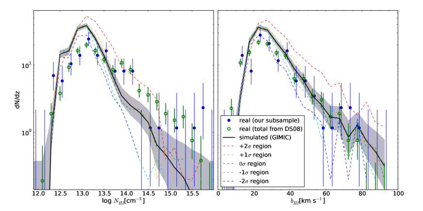
Figure 5: Redshift number density of H i lines as a function of both column density (left panel) and Doppler parameter (right panel) using abritrary binning of $\Delta\log N_{\rm HI}=0.2$ dex and $\Delta b_{\rm HI}=5$ km s^-1 respectively. Both results have not been corrected for incompleteness. Green open-circles correspond to real data from the total sample of DS08 ($657$ systems) while blue filled-circles (slightly offset in the $x$-axes for clarity) correspond to the subsample used in this study ($106$ systems). The black line corresponds to the volume-weighted result from the combination of the five gimic regions where the shaded region correspond to the $\pm 1\sigma$ uncertainty. Dashed lines show the results from each individual gimic region. Error bars correspond to the Poissonian uncertainty from the analytical approximation $\sigma^{+}_{n}\approx\sqrt{n+\frac{3}{4}}+1$ and $\sigma^{-}_{n}\approx\sqrt{n-\frac{1}{4}}$ (Gehrels, 1986).

The fraction of hydrogen in the form of H i within gimic is obtained from cloudy (Ferland et al., 1998) after assuming an ionization background from Haardt & Madau (1996) that yields a photo-ionization rate $\Gamma=8.59\ 10^{-14}$ s^-1. This ionization background is not well constrained at $z\approx 0$, so we use a post processing correction to account for this uncertainty. In the optically thin regime $\Gamma^{\rm thin}\propto\frac{1}{\tau}$, where $\tau$ is the optical depth (Gunn & Peterson, 1965). Then, scaling the optical depth values is equivalent to scaling the ionization background (e.g., Theuns et al., 1998a; Davé et al., 1999). First, we combined the five gimic regions using different volume weights namely: $(1/12,1/6,1/2,1/6,1/12)$ for the $(-2,-1,0,+1,+2)\sigma$ regions respectively (see Appendix 2 in Crain et al., 2009, for a justification of these weights). Then, we searched for a constant value to scale all the original optical depth values such that the mean flux of the combined sample is equal to the observed mean flux of Ly-$\alpha$ absorption at low redshift. A second possibility is to scale the optical depth values in order to match the redshift number density of H i lines in some column density range, $dN/dz$, instead of the mean flux. Ideally by matching one observable the second would be also matched.

Extrapolating the double power-law fit result from Kirkman et al. (2007) to $z=0$ (see their equation $6$), the observed mean flux is $\langle F\rangle=0.987$ with a typical statistical uncertainty of $\sigma_{\langle F\rangle}\sim 0.003$. In order to match this number in the simulation a scale of $1.16$ is required in the original optical depth values ($0.86$ in $\Gamma$). From this correction, the redshift number density of lines in the range $10^{13.2}\leq N_{\rm HI}\leq 10^{14}$ cm^-2 is found to be $dN/dz\approx 50$. For reference, Lehner et al. (2007) and DS08 found $dN/dz\sim 50-90$ over the same column density range. We have repeated the experiment for consistency, using $\langle F\rangle=\{0.984,0.990\}$ which are within $\pm 1\sigma_{\langle F\rangle}$ of the extrapolated value. To match these, scales of $1.50$ and $0.84$ are required in the original optical depths values respectively ($0.67$ and $1.19$ in $\Gamma$). From those mean fluxes we found $dN/dz\approx\{70,35\}$ respectively along the same column density range. Therefore, a value of $\langle F\rangle=0.990$ underpredicts the number of H i lines. On the other hand, values of $\langle F\rangle=0.987$ and $0.984$ are in good agreement with observations. In the following analysis we use $\langle F\rangle=0.987$ unless otherwise stated.

4.2 Comparison between simulated and observed H i properties

Figure 5 shows the redshift number density of H i lines (not corrected for incompleteness) as a function of both column density (left panel) and Doppler parameter (right panel). Data from the simulation are shown by the black line (volume-weighted result) and each individual gimic region is shown separately by the dashed lines. For comparison, data from observations are also shown. Green open-circles correspond to the total sample from DS08 ($657$ systems) while blue filled-circles correspond to the subsample used in this study ($106$ systems that intersect the SDSS volume). There is not perfect agreement between simulated and real data. We see an excess (lack) of systems with $N_{\rm HI}$ $\lesssim 10^{13.5}$ cm^-2 ($N_{\rm HI}$ $\gtrsim 10^{14}$ cm^-2) in the simulation compared to observations while Doppler parameters are in closer agreement, although there is still a difference at low $b_{\rm HI}$.

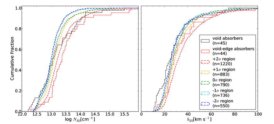
Figure 6: Column density (left panel) and Doppler parameter (right panel) cumulative distributions for H i. Void absorbers are shown by solid-black lines while void-edge absorbers are shown by solid-red lines. Dashed lines show the result from each individual gimic region. For simplicity we only show LSS definitions based on $X$.

Assuming that the column density distribution can be modeled as a power-law, the position of the turnover at the low $N_{\rm HI}$ end give us an estimation of the completeness level of detection in the sample. As the turnover appears to be around $N_{\rm HI}$ $\approx 10^{13}$ cm^-2 in both simulated and real data (by design) we do not, in principle, attribute the discrepancy in the column-density distributions to a wrong choice of the simulated $S/N$. Raising the mean flux to a greater value than $\langle F\rangle=0.987$ (less absorption) does not help as the $dN/dz$ in the range $10^{13.2}\leq N_{\rm HI}\leq 10^{14}$ cm^-2 will then be smaller than the observational result (see §4.1). We attempted to get a better match by using a mean flux of $\langle F\rangle=0.984$ (more absorption), motivated to produce a better agreement at higher column densities. In order to agree at low column densities, we had to degrade the sample $S/N$ to be composed of $\sim 400$, $\sim 100$ and $\sim 500$ sightlines at signal-to-noise ratios of $9$, $23$ and $2$ respectively. It is implausible that half of the observed redshift path has such poor quality.

Another possibility to explain the discrepancy could be the fact that weak systems in observations were preferentially characterized with the AOD method, whereas here we have only used Voigt profile fitting. In order to test this hypothesis, we have merged closely separated systems (within $150$ km s^-1) whose summed column density is less than $10^{13.5}$ cm^-2. Using these constraints, $43$ out of $4179$ systems were merged ($\approx 1\%$). Such a small fraction does not have an appreciable effect on the discrepancy. As an extreme case, we have repeated the experiment merging all systems within $300$ km s^-1 independently of their column densities. From this, $555$ out of $4179$ systems were merged ($\approx 13\%$) but still it was not enough to fully correct the discrepancy. Given that the discrepancy is not explained by a systematic effect from different line characterization methods, we chose to keep our original simulated sample in the following analysis without merging any systems.

There is a reported systematic effect by which column densities inferred from a single Ly-$\alpha$ line are typically (with large scatter) underestimated with respect to the curve-of-growth (COG) solution. Similarly $b_{\rm HI}$ are typically overestimated (Shull et al. 2000; Danforth et al. 2006; see also Appendix A.2 for discussion on how this may affect our observational results). This effect is only appreciable for $N_{\rm HI}$ $\gtrsim 10^{14}$ cm^-2 and is bigger for saturated lines. Given that our simulated sample was constructed to reproduce the observed sample, this effect could be present. If so, it would in principle help to reduce the discrepancy at the high column density end. From figure 3 of Danforth et al. (2006) we have inferred a correction for systems with $N_{\rm HI}$ $\geq 10^{13.5}$ cm^-2 of,

$$\log N_{\rm HI}^{\rm corr}=\frac{\log N_{\rm HI}^{\rm obs}-8.37}{1-0.62}\ \rm{,}$$ (3)

where $N_{\rm HI}^{\rm corr}$ and $N_{\rm HI}^{\rm obs}$ are the corrected and observed $N_{\rm HI}$ values respectively. From this correction we found an increase in the number of systems at $N_{\rm HI}$ $\gtrsim 10^{14.5}$ cm^-2 up to values consistent with observations. This however does not help with the discrepancy at lower column densities.

At this point, it is difficult to reconcile the simulation result with the real data using only a single effect. We note that the discrepancy is a factor of $\sim 2$ only, so it could be in principle explained through a combination of several observational effects. Also note that the number of observed lines at higher column densities is still small and it could be affected by low number statistics. The lack of systems with very low $N_{\rm HI}$ and $b_{\rm HI}$ values can be explained by our selection of the highest signal-to-noise being $S/N=23$ while in real data there could be regions with higher values. It is not the aim of this section to have a perfect match between simulations and observations but rather examine the qualitative differences between simulated regions of different densities. Thus hereafter, we will use the results from the simulation in its original form (as shown in Figure 5), i.e., without any of the aforementioned corrections.

4.3 Simulated H i absorbers properties in different LSS regions

Given that gimic does not provide enough volume to perform a completely analogous search for voids (each region is $\sim 20$ $h^{-1}$Mpc of radius), we use them only as crude guides to compare our results with. We could consider the $-2\sigma$ region as representative of void regions as it is actually centered in one. Naively, we could consider the $0\sigma$ regions as representative of void-edge regions, as it is there where the mean cosmological density is reached. A direct association for the $+1\sigma$ and $+2\sigma$ is not so simple though, as they would be associated to some portions of the void-edge regions too. It seems more reasonable to use the gimic spheres as representative of different density environments then, where $-2\sigma$/$+2\sigma$ correspond to extremely under/over-dense regions and so on. For reference, the whole $(-2,-1,0,+1,+2)\sigma$ gimic regions correspond to densities of $\frac{\rho}{\langle\rho\rangle}\approx(0.4,0.6,0.9,1.2,1.8)$ at $z=0$ respectively, where $\langle\rho\rangle$ is the mean density of the universe (see Figure A1 from Crain et al., 2009).

Figure 6 shows the cumulative distributions of $N_{\rm HI}$ (left panel) and $b_{\rm HI}$ (right panel). Results from each of the individual gimic region are shown by dashed lines. Void and void-edge absorbers are shown by solid black and red lines respectively. For simplicity we show only LSS definition based on $X$. Cumulative distributions between real and simulated data do not agree perfectly. However, in both real and simulated data, there is an offset between column densities and Doppler parameters found in different environments. Low density environments have smaller values for both $N_{\rm HI}$ and $b_{\rm HI}$ than higher density ones (and viceversa). This trend still holds when using a $S/N=23$ per pixel for the $5000$ sightlines.

Table 4: Kolmogorov-Smirnov (KS) test probabilities between different gimic regions.

	$-2\sigma$	$-1\sigma$	$\ 0\sigma$	$+1\sigma$	$+2\sigma$
$-2\sigma$		$30\%$	$2\%$	$2\%$	$\ll 1\%$
$-1\sigma$	$77\%$		$6\%$	$\ll 1\%$	$\ll 1\%$
$0\sigma$	$11\%$	$0.9\%$		$0.7\%$	$\ll 1\%$
$+1\sigma$	$\ll 1\%$	$\ll 1\%$	$0.4\%$		$\ll 1\%$
$+2\sigma$	$\ll 1\%$	$\ll 1\%$	$\ll 1\%$	$\ll 1\%$

The KS test gives a significant difference between the $+2\sigma$, $+1\sigma$ and $+0\sigma$ regions, and any other gimic region at the $\gg 99\%$, $\gtrsim 99\%$ and $\gtrsim 95\%$ confidence level respectively in both $N_{\rm HI}$ and $b_{\rm HI}$ distributions. The KS test gives no significant difference between the $-2\sigma$ and $-1\sigma$ regions in both $N_{\rm HI}$ and $b_{\rm HI}$ distributions (see Table 4). These results do not change significantly when correcting gimic to match the observed $N_{\rm HI}$ distribution using a different $\langle F\rangle$ and $S/N$ values. We do not attempt to make a more detailed comparison between distributions coming from real data (void, void-edge samples) and the different gimic regions as there are already known differences between them (see §4.2).

5 Discussion

5.1 Three Ly-$\alpha$ forest populations

Our first result is that there is a $>99\%$ c.l. excess of Ly-$\alpha$ systems at the edges of galaxy voids compared to a random distribution (see §3.1 and Figure 1). Our random sample was normalized to have the same density of systems in the whole volume. Then, an excess in a sub-volume means necessarily a deficit in another. Given that we found no significant difference in the number of systems in voids with respect to the random expectation, the excess is not explained by a deficit of Ly-$\alpha$ systems inside galaxy voids. The observed excess seems more related to the lack of systems found at distances $\gtrsim 5$ $h^{-1}$Mpc outside the cataloged voids (and viceversa). Thus, despite the fact that we see Ly-$\alpha$ clustered at the edges of galaxy voids, it is not clear from this data that Ly-$\alpha$-voids at low-$z$ exist at all (see Carswell & Rees 1987 for similar result at high-$z$; although see Williger et al. 2000). This picture is somewhat different from the case of galaxies, where galaxy voids are present even in the distribution of low mass galaxies (e.g., Peebles, 2001; Tikhonov & Klypin, 2009). There is agreement though in the sense that both Ly-$\alpha$ system and galaxy distributions have their peaks at the edges of galaxy voids. We observe a typical scale length of the excess to be $\sim 5$ $h^{-1}$Mpc, consistent with numerical predictions for the typical radius of the filamentary structure of the ‘cosmic web’ ($\sim 2$ $h^{-1}$Mpc; see González & Padilla, 2010; Aragón-Calvo et al., 2010; Bond et al., 2010). Note that this scale length is approximately twice the scale associated with a velocity uncertainty of $\Delta v\approx 200$ km s^-1 at $z=0$. Such dispersions could be present in our void-edge sample.

In our data analysis we have defined three samples of absorption systems, based on how they are located with respect to the closest galaxy void (see §3.2). Let us consider now a very simple model in which we have only two LSS environments: under-dense and over-dense LSS. Then we could relate all the ‘random-like’ Ly-$\alpha$ forest systems found in the void sample ($X<0.9$ and/or $D<-2$ $h^{-1}$Mpc) with the under-dense LSS, while all the systems associated with the excess over random ($0.9\leq X<1.3$ and/or $-2\leq D<4$ $h^{-1}$Mpc) to the over-dense LSS. Note that the fact that we cannot distinguish between the under-dense LSS Ly-$\alpha$ distribution and a random distribution does not mean that the former is really random. If these Ly-$\alpha$ forest systems follow the underlying dark matter distribution (e.g., see Croft et al., 1998), they should have a non-negligible clustering amplitude that is not observed only because of the lack of statistical power of our sample. In relative terms, considering the under-dense LSS Ly-$\alpha$ as random seems to be a good approximation though, especially for the large scale distances involved in this work ($>1$ Mpc). This is also supported by the very low auto-correlation amplitude observed in the whole population of Ly-$\alpha$ forest systems at such scales (e.g., Croft et al., 1998; Rollinde et al., 2003; Crighton et al., 2011). This ‘random’ behavior of Ly-$\alpha$ systems in the under-dense LSS can be understood as originating in structures still evolving from the primordial density perturbations in the linear regime. At $z=0$ however, the majority of the mass resides at the edges of voids (in the ‘cosmic web’) whose density perturbations have reached non-linear evolution regime at higher redshifts. For reference, we expect the under-dense and over-dense LSS to have typical $\delta\gtrsim 0$ and $\delta\lesssim 0$ respectively, where $\delta$ is the density contrast defined as,

$$$$\delta\equiv\frac{\rho-\langle\rho\rangle}{\langle\rho\rangle}\ \ \rm{,}$ $$$ (4)

where $\rho$ is the density and $\langle\rho\rangle$ is the mean density of the universe. Note however that these LSS environments are not defined by a particular density but rather by a topology (voids, walls, filaments).

Theoretical arguments point out that the observed column density of neutral hydrogen at a fixed $z$ is,

$$N_{\rm HI}\propto\rho_{\rm H}^{1.5}\ T^{-0.26}\ \Gamma^{-1}\ f_{g}^{0.5}\ \ \rm{,}$$ (5)

where $\rho_{\rm H}$ is the density of hydrogen, $T$ is the temperature of the gas, $\Gamma$ is the hydrogen photo-ionization rate and $f_{g}$ is the fraction of mass in gas (Schaye, 2001). In the diffuse IGM it has been predicted that $T\propto\rho_{\rm H}^{\alpha}$, where $\alpha\approx 0.59$ (Hui & Gnedin, 1997). This implies that for a fixed $\Gamma$, the main dependence of $N_{\rm HI}$ is due to $\rho_{\rm H}$ as $N_{\rm HI}$ $\propto\rho_{\rm H}^{1.4}$. Then, despite the extremely low densities inside galaxy voids we can still observe Ly-$\alpha$ systems, although only the ones corresponding to the densest structures.

Let us consider the predicted ratio between $N_{\rm HI}$ observed inside voids and at the edges of voids as,

$$\frac{N_{\rm HI}^{\rm void}}{N_{\rm HI}^{\rm edge}}\approx\left(\frac{\rho_{\rm H}^{\rm void}}{\rho_{\rm H}^{\rm edge}}\right)^{1.4}\left(\frac{\Gamma^{\rm void}}{\Gamma^{\rm edge}}\right)^{-1}\left(\frac{f_{g}^{\rm void}}{f_{g}^{\rm edge}}\right)^{0.5}\ \ \rm{.}$$ (6)

Given that the timescale for photons to travel along $\sim 10-20$ $h^{-1}$Mpc is $\ll 1$ Gyr, we can consider $\Gamma^{\rm void}\approx\Gamma^{\rm edge}$. Even if we assume that the gas inside voids has not formed galaxies, $f_{g}^{\rm void}\gtrsim f_{g}^{\rm edge}$, because $f_{g}$ is dominated by the dark matter. This implies that a given observed $N_{\rm HI}$ inside and at the edge of galaxy voids will correspond to similar densities of hydrogen ($\rho^{\rm void}_{\rm H}\approx\rho^{\rm edge}_{\rm H}$). This is important because it means that the Ly-$\alpha$ forest in the under-dense LSS is not different than the over-dense LSS one, and two systems with equal $N_{\rm HI}$ are comparable, independently of its large scale environment.

If there were no galaxies, this simple model may suffice to explain the differences in the observed Ly-$\alpha$ population. The fact that some of the Ly-$\alpha$ systems are directly associated with galaxies cannot be neglected though. There is strong evidence from observations (e.g., Lanzetta et al., 1995; Chen et al., 1998; Stocke et al., 2006; Morris & Jannuzi, 2006; Chen & Mulchaey, 2009; Crighton et al., 2011; Prochaska et al., 2011; Rakic et al., 2011; Rudie et al., 2012) and simulations (e.g., Fumagalli et al., 2011; Stinson et al., 2011) that $N_{\rm HI}\gtrsim 10^{15}$ cm^-2 systems are preferentially found within a couple of hundred kpc of galaxies. Probably an appropriate interpretation of such a result is that galaxies are always found in ‘local’ ($\lesssim 100$ $h^{-1}$kpc) high $N_{\rm HI}$ density regions. Then, a plausible scenario would require at least three types of Ly-$\alpha$ forest systems: (1) containing embedded galaxies, (2) associated with over-dense LSS but with no close galaxy and (3) associated with under-dense LSS but with no close galaxy. For convenience, we will refer to the first type as ‘halo-like’, although with the caution that these systems may not be gravitationally bound with the galaxy.

Given that there are galaxies inside galaxy voids, the ‘halo-like’ Ly-$\alpha$ systems will be present in both low and high density LSS environments (galaxies are a ‘local’ phenomenon). The contribution of the ‘halo-like’ in galaxy voids could be considered small though. Assuming this contribution to be negligible, we can estimate the fraction of Ly-$\alpha$ systems in the under-dense LSS as $\approx 25-30\%\pm 6\%$. Likewise, $\approx 70-75\%\pm 12\%$ of the Ly-$\alpha$ forest population are due to a combination of systems associated with galaxies and systems associated with the over-dense LSS. We could estimate the contribution of ‘halo-like’ absorbers by directly looking for and counting galaxies relatively close to the absorption systems. A rough estimation can be done by assuming that galaxy halos will have only $N_{\rm HI}\geq 10^{14}$ cm^-2 systems, leading to a contribution of $\approx 12-15\%\pm 4\%$ in our sample.

In summary, our results require at least three types of Ly-$\alpha$ systems to explain the observed Ly-$\alpha$ forest population at low-$z$ ($N_{\rm HI}$ $\gtrsim 10^{12.5}$ cm^-2):

• Halo-like: Ly-$\alpha$ with embedded nearby galaxies ($\lesssim 100$ $h^{-1}$kpc) and so directly correlated with galaxies ($\approx 12-15\%\pm 4\%$),

• Over-dense LSS: Ly-$\alpha$ associated with the over-dense LSS that are correlated with galaxies only because both populations lie in the same LSS regions ($\approx 50-55\%\pm 13\%$) and,

• Under-dense LSS: Ly-$\alpha$ associated with the under-dense LSS with very low auto-correlation amplitude that are not correlated with galaxies ($\approx 25-30\%\pm 6\%$).

The relative contributions of these different Ly-$\alpha$ populations is a function of the lower $N_{\rm HI}$ limit. Low $N_{\rm HI}$ systems dominate the Ly-$\alpha$ column density distribution. Then, given that under-dense LSS Ly-$\alpha$ systems tend to be of lower column density than the other two types, we expect the contribution of ‘random-like’ Ly-$\alpha$ to increase (decrease) while observing at lower (higher) $N_{\rm HI}$ limits. Note that there are not sharp $N_{\rm HI}$ limits to differentiate between our three populations (see Figure 2). The ‘halo-like’ is defined by being close to galaxies while the ‘LSS-like’ ones are defined in terms of a LSS topology (voids, wall, filaments).

Motivated by a recently published study on the Ly-$\alpha$/galaxy association by Prochaska et al. (2011), we can set a conservative upper limit to the ‘halo-like’ contribution. These authors have found that nearly all their observed $L\geq 0.01L^{*}$ galaxies ($33/37$) have $N_{\rm HI}$ $\geq 10^{13.5}$ cm^-2 absorption at impact parameters $<300$ $h^{-1}_{72}$kpc. If we invert the reasoning and assume an extreme (likely unrealistic) scenario where all the $N_{\rm HI}$ $\geq 10^{13.5}$ cm^-2 are directly associated with galaxies, then, the ‘halo-like’ contribution will have an upper limit of $<33\%\pm 7\%$. Consequently, the contribution of the over-dense LSS to the Ly-$\alpha$ population will be $>37-42\%\pm 14\%$. Still, note that we have found several systems with $10^{13.5}\lesssim N_{\rm HI}\lesssim 10^{14.5}$ cm^-2 inside galaxy voids for which a direct association with galaxies is dubious (see Figure 2). Also note that only $\sim 10\%$ ($\sim 0\%$) of the Ly-$\alpha$ systems between $10^{13.5}<N_{\rm HI}<10^{14.5}$ cm^-2 may be associated with a galaxy at impact parameters $<300$ kpc ($<100$ kpc) in the Prochaska et al. (2011) sample (see their figure 4).

Our findings are consistent with previous studies pointing out a non-negligible contribution of ‘random’ Ly-$\alpha$ systems (at a similar $N_{\rm HI}$ limit) of $\approx 20-30\%$ (Mo & Morris, 1994; Stocke et al., 1995; Penton et al., 2002). These authors estimated that $\approx 70-80\%$ of the Ly-$\alpha$ population is associated with either LSS (galaxy filaments) or galaxies. Note that Mo & Morris (1994) put a upper limit of $\approx 20\%$ being directly associated with galaxies, which is also consistent with our estimation. Our result is also in accordance with the previous estimation that $22\%\pm 8\%$ (Penton et al. 2002; based on $8$ systems) and $17\%\pm 4\%$ (Wakker & Savage 2009; based on $17$ systems) of the Ly-$\alpha$ systems lie in voids (defined as locations at $>3$ $h^{-1}_{70}$ Mpc from the closest $>L^{*}$ galaxy). This is in contrast with early models that associated all Ly-$\alpha$ systems with galaxies (e.g., Lanzetta et al., 1995; Chen et al., 1998).

Although there is general agreement with recently proposed models to explain the origin of the low-$z$ Ly-$\alpha$ forest (e.g., Wakker & Savage, 2009; Prochaska et al., 2011), we emphasize that our interpretation is qualitatively different and adds an important component to the picture: the presence of the under-dense LSS (‘random-like’) systems. For instance, assuming infinite filaments of typical widths of $\approx 400$ $h^{-1}_{72}$kpc around galaxies, Prochaska et al. (2011) argued that all Ly-$\alpha$ systems at low-$z$ belong either to the circum-galactic medium (CGM; which includes our ‘galaxy halo’ definition) or the filamentary structure in which galaxies reside (equivalent to our over-dense LSS definition). Our findings are not fully consistent with this hypothesis, as neither the ‘CGM model’ nor the ‘galaxy filament model’ seem likely to explain the majority of our under-dense LSS absorbers at $N_{\rm HI}$ $\lesssim 10^{13.5}$ cm^-2. To do so there would need to be a whole population of unobserved galaxies (dwarf spheroidals?) inside galaxy voids with an auto-correlation amplitude as low as the ‘random-like’ Ly-$\alpha$ one. As discussed by Tikhonov & Klypin 2009, very low surface brightness dwarf spheroidals could be a more likely explanation than dwarf irregulars because the latter should have been observed with higher incidences in recent H i emission blind surveys inside galaxy voids (e.g., HIPASS, Doyle et al. 2005). On the other hand, the formation of dwarf spheroidals inside galaxy voids is difficult to be explained from the current galaxy formation paradigm (see Tikhonov & Klypin 2009 for further discussion). As mentioned, it seems more natural to relate the majority of the under-dense LSS absorbers with the peaks of extremely low density structures inside galaxy voids, still evolving linearly from the primordial density perturbations that have not formed yet galaxies because of their low densities. Our interpretation can be tested by searching for galaxies close to our lowest $N_{\rm HI}$ void-absorbers (see Figure 2). Another prediction of our interpretation is that the vast majority of $N_{\rm HI}$ $\lesssim 10^{13}$ cm^-2 systems should reside inside galaxy voids. If the QSO sightlines used here were observed at higher sensitivities, weak Ly-$\alpha$ systems should preferentially appear at $X<1$ ($D<0$ $h^{-1}$Mpc). Therefore, we should expect to have an anti-correlation between $N_{\rm HI}$ $\lesssim 10^{13}$ cm^-2 and galaxies.

5.2 $N_{\rm HI}$ and $b_{\rm HI}$ distributions

Our second result is that there is a systematic difference ($\gtrsim 98\%$ c.l.) between the column density distributions of Ly-$\alpha$ systems found within, and those found at the edge of, galaxy voids. Void absorbers have more low column density systems than the void-edge sample (see Figure 3). A similar trend is found in gimic, where low density environments present smaller $N_{\rm HI}$ values than higher density ones (see Figure 6, left panel). This can be explained by the fact that baryonic matter follows the underlying dark matter distribution. Then, the highest density environments should be located at the edges of voids (in the intersection of walls and filaments), consequently producing higher column density absorption than in galaxy voids (e.g., see Schaye, 2001).

Also, by construction, there is a higher chance to find galaxies at the edges rather than inside galaxy voids. Assuming that some of the Ly-$\alpha$ forest are associated with galaxy halos (see §5.1 for further discussion), then this population should be present mainly in our void-edge sample. As galaxy halos correspond to local density peaks, we should also expect on average higher column density systems in this population. Given that galaxies may affect the properties of the surrounding gas, there could be processes that only affect Ly-$\alpha$ systems close to galaxies. For instance, the distribution of Ly-$\alpha$ systems around galaxy voids seems to show a two-peaked shape (see Figure 1). We speculate that this could be a signature of neutral hydrogen being ionized by the ultra-violet background produced by galaxies (see also Adelberger et al., 2003), mostly affecting $N_{\rm HI}$ $\lesssim 10^{13}$ cm^-2 inside the filamentary structure of the ‘cosmic web’. Another explanation could be that in the inner parts of the filamentary structure, Ly-$\alpha$ systems get shock heated by the large gravitational potentials, raising their temperature and ionization state (e.g., Cen & Ostriker, 1999). A third possibility is that it could be a signature of bulk outflows as the shift between peaks is consistent with a $\Delta v\approx 200-300$ km s^-1. On the other hand, the two peaks could have distinct origins as the first one may be related to an excess of $N_{\rm HI}$ $\lesssim 10^{13}$ cm^-2 systems, probably associated with the over-dense LSS in which galaxies reside, while the second one may be related to an excess of $N_{\rm HI}$ $\gtrsim 10^{14}$ cm^-2 systems, more likely associated with systems having embedded galaxies. As mentioned, we cannot prove the reality of this two-peaked signature at a high confidence level from the current sample and so we leave to future studies the confirmation or disproof of these hypotheses.

The gimic data analysis shows a clear differentiation of $b_{\rm HI}$ distributions in different density environments (see Figure 6, right panel). Low density environments have smaller $b_{\rm HI}$ values than higher density ones. We see a similar trend in the real data between our void and void-edge absorber samples, although only at a $\gtrsim 90\%$ of confidence level (i.e., not very significant; see Figure 4). The main mechanisms that contribute to the observed line broadening are temperature, local turbulence and bulk motions of the gas (excluding systematic effects from the line fitting process or degeneracy with $N_{\rm HI}$ for saturated lines). Naturally, in high density environments, we would expect to have greater contributions from both local turbulence and bulk motions compared to low density ones. The gas temperature is also expected to increase from low density environments to high density ones. As previously mentioned, theoretical arguments predict the majority of the diffuse IGM will have temperatures related to the density by $T\propto\rho^{\alpha}$ with $\alpha>0$ (Hui & Gnedin, 1997; Theuns et al., 1998b; Schaye et al., 1999). This is also seen in density-temperature diagrams drawn from current hydrodynamical cosmological simulations (e.g., Davé et al., 2010; Tepper-García et al., 2012). Therefore, our findings are consistent with current expectations.

5.3 Future work

The high sensitivity of the recently installed Cosmic Origins Spectrograph (COS/HST, Green et al., 2012) in the UV (especially the far-UV), will allow us to improve the $N_{\rm HI}$ completeness limit compared with current surveys. This will considerably increase the number of observed Ly-$\alpha$ absorption systems at low-$z$. In the short term, there are several new QSO sightlines scheduled for observations (or already observed) with COS/HST that intersect the SDSS volume. Combining these with current and future galaxy void catalogs, we expect to increase the statistical significance of the results presented in this work. COS/HST will also allow observations of considerably more metal lines (especially O vi) than current IGM surveys. Again, in combination with LSS surveys, this will be very useful for studies on metal enrichment in different environments. For instance, we have identified $8$ systems with observed O vi absorption from STIS/HST in our sample. Three of these lie inside voids at $X\approx\{0.6,0.7,0.9\}$ ($D\approx\{-5.4,-4.6,-1.6\}$ $h^{-1}$Mpc) respectively. The first two systems that lie inside voids correspond to the highest $N_{\rm HI}$ values ($N_{\rm HI}$$>10^{14.5}$ cm^-2; see Figure 2). We have performed a search in the SDSS DR8 for galaxies in a cylinder of radius $1$ $h^{-1}_{71}$ Mpc and within $\pm 200$ km s^-1 around these $2$ absorbers (both systems belong to the same sightline and are at a similar redshift; one of them shows C iv absorption also). We found $9$ galaxies with these constraints, hinting on a possible association of these systems with a void galaxy. The one at the very edge of the void limit has $N_{\rm HI}$ $=10^{13.14\pm 0.07}$ cm^-2 and $N_{\rm OVI}=10^{13.69\pm 0.18}$ cm^-2, and it could in principle be associated with the over-dense LSS. The other $5$ O vi absorbers lie in our void-edge sample and have $N_{\rm HI}$ $>10^{13.5}$ cm^-2, so they are likely to be associated with galaxies. None of the observed O vi lie in our unclassified sample. The current sample of O vi systems is very small, and so we do not aim to draw statistical conclusions from them. However, these systems individually offer interesting cases worth further investigation. We intend to perform a carefully search for galaxies that could be associated to each of the Ly-$\alpha$ absorbers presented in our sample in future work. In the longer term, it will be possible to extend similar analysis to well defined galaxy filaments and clusters when the new generation of galaxy surveys are released.

A scenario with three different types of Ly-$\alpha$ forest systems, as proposed here, can help to interpret recent measurements of the cross-correlation between Ly-$\alpha$ and galaxies (Chen et al., 2005; Ryan-Weber, 2006; Wilman et al., 2007; Chen & Mulchaey, 2009; Shone et al., 2010; Rudie et al., 2012). These studies come mainly from pencil beam galaxy surveys around QSO sightlines where identifying LSS such as voids or filaments is more challenging. As mentioned, different Ly-$\alpha$ systems are not separated by well defined $N_{\rm HI}$ limits and so we suggest using our results to properly account for under-dense LSS (‘random-like’) absorbers in gas/galaxy cross-correlations. Truly random distributions are easy to correct for, as they lower the amplitude of the correlations at all scales. Then, acknowledging these ‘random-like’ absorbers, it will be possible to split the correlation power in its other two main components: gas in galaxy halos and gas in the over-dense LSS. Our group is currently working in a future paper to study the gas/galaxy cross-correlation, in which these corrections will be taken into account.

6 Summary

We have presented a statistical study of H i Ly-$\alpha$ absorption systems found within and around galaxy voids at $z\lesssim 0.1$. We found a significant excess ($>99\%$ c.l.) of Ly-$\alpha$ systems at the edges of galaxy voids with respect to a random distribution, over a $\sim 5$ $h^{-1}$Mpc scale. We have interpreted this excess as being due to Ly-$\alpha$ systems associated with both galaxies (‘halo-like’) and the over-dense LSS in where galaxies reside (the observed ‘cosmic web’), accounting for $\approx 70-75\%\pm 12\%$ of the Ly-$\alpha$ population. We found no significant difference in the number of systems inside galaxy voids compared to the random expectation. We therefore infer the presence of a third type of Ly-$\alpha$ systems associated to the under-dense LSS with a low auto-correlation amplitude ($\approx$ random) that are not associated with luminous galaxies. These ‘random-like’ absorbers are mainly found in galaxy voids. We argue that these systems can be associated with structures still growing linearly from the primordial density fluctuations at $z=0$ that have not yet formed galaxies because of their low densities. Although the presence of a ‘random’ population of Ly-$\alpha$ absorbers was also inferred (or assumed) in previous studies, our work presents for the first time a simple model to explain it (see §5.1). Above a limit of $N_{\rm HI}$ $\gtrsim 10^{12.5}$ cm^-2, we estimate that $\approx 25-30\%\pm 6\%$ of Ly-$\alpha$ forest systems are ‘random-like’ and not correlated with luminous galaxies. Assuming that only $N_{\rm HI}$ $\geq 10^{14}$ cm^-2 systems have embedded galaxies nearby, we have estimated the contribution of the ‘halo-like’ Ly-$\alpha$ population to be $\approx 12-15\%\pm 4\%$ and consequently $\approx 50-55\%\pm 13\%$ of the Ly-$\alpha$ systems to be associated with the over-dense LSS.

We have reported differences between both the column density ($N_{\rm HI}$) and the Doppler parameter ($b_{\rm HI}$) distributions of Ly-$\alpha$ systems found inside and at the edge of galaxy voids observed at the $>98\%$ and $>90\%$ of confidence level respectively. Low density environments (voids) have smaller values for both $N_{\rm HI}$ and $b_{\rm HI}$ than higher density ones (edges of voids). These trends are theoretically expected. We have performed a similar analysis using simulated data from gimic, a state-of-the-art hydrodynamical cosmological simulation. Although gimic did not give a perfect match to the observed column density distribution, the aforementioned trends were also seen. Any discrepancy between gimic and real data could be due to low number statistic fluctuations and/or a combination of several observational effects.

In summary, our results are consistent with the expectation that the mechanisms shaping the properties of the Ly-$\alpha$ forest are different in different LSS environments. By focusing on a ‘large scale’ ($\gtrsim 10$ Mpc) point of view, our results offer a good complement to previous studies on the IGM/galaxy connection based on ‘local’ scales ($\lesssim 2$ Mpc).

Appendix A Check for systematic effects

In this section we investigate possible biases or systematic effects that could be present in the data analysis.

A.1 Comparison between our subsample and the whole DS08 sample

In this section we explore whether the subsample of H i systems used here is statistically different from the rest of the H i population found in the other sightlines of the DS08 catalog. For this, we compared the column density ($N_{\rm HI}$) and Doppler parameter ($b_{\rm HI}$) distributions between the $106$ absorption systems found inside the void catalog volume ($0.01\leq z_{\rm abs}\leq 0.102$ in $11$ sightlines) with those $545$ outside this volume. The KS test gives a probability of $\approx 5\%$ and $\approx 90\%$ that both $N_{\rm HI}$ and $b_{\rm HI}$ distributions, inside and outside the void catalog volume, are drawn from the same parent distribution respectively. This shows there is no significant difference in the $b_{\rm HI}$ distribution and an $\approx 2\sigma$ difference between the $N_{\rm HI}$ distributions.

One explanation for such a difference could be due to an intrinsic evolution of the Ly-$\alpha$ forest between $z_{\rm abs}\lesssim 0.102$ and $0.102\lesssim z_{\rm abs}<0.4$. To check this, we performed a KS comparison between the $286$ absorbers at $z_{\rm abs}<0.102$ (regardless of whether they are inside the void catalog volume or not) with the $365$ systems at higher redshifts, to look for a possible difference in both $N_{\rm HI}$ and $b_{\rm HI}$ distributions. The distribution of $b_{\rm HI}$ does not show any difference (KS Prob. $\approx 87\%$). On the other hand, the KS probability for the two $N_{\rm HI}$ distributions is $\approx 8\%$, hinting that such evolution could be present. We note, however, that an observational bias between low and high-$z$ systems (e.g., due to different selection functions) could also explain the observed difference. We did not further explore this matter.

Finally, we repeated the previous comparisons between the $106$ systems inside the void catalog volume with those $155$ outside it having $0.01\leq z_{\rm abs}\leq 0.102$. The KS test gives this time a probability of $\approx 23\%$ and $\approx 81\%$ of both $N_{\rm HI}$ and $b_{\rm HI}$ inside and outside the void catalog volume are drawn from the same parent distribution, respectively. No significant ($>2\sigma$) differences are found for these samples. Thus, we conclude that the properties of the systems in the sightlines used in this work are not statistically different from the properties of the systems in other sightlines when we restrict ourselves to the same redshift range.

We note that for our comparisons we use systems with $N_{\rm HI}$ below the completeness of the column density distribution itself ($N_{\rm HI}\lesssim 10^{13.4}$ cm^-2). The classification of absorber environment does not depend on column density but rather corresponds to a geometrical association of absorbers with known galaxy voids. Therefore, this should not affect any of our results. We also checked that none of the AGN used here were observed in particular for having sightlines intersecting a known void region.

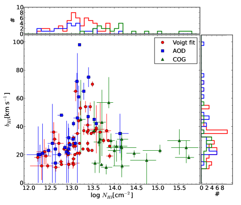
Figure 7: H i column density versus H i Doppler parameter for systems in our sample. Different characterization methods (see §A.2) are shown by different colors/symbols. Red circles correspond to systems measured by Voigt profile fits. Blue squares correspond to systems measured by the AOD method. Green triangles correspond to systems measured by a COG solution. Histograms (arbitrary binning) are also shown around the main panel using the previous color definition.

A.2 Systematics in the DS08 characterization method

A particular source of concern is the fact that DS08 used different methods for obtaining the H i column densities and Doppler parameters in the catalog. They used curve-of-growth (COG) solutions when other Lyman series lines were available other than Ly-$\alpha$. For the rest of the systems they used either a single Voigt profile fit (preferentially for strong or blended lines) and/or the apparent optical depth method (AODM, Savage & Sembach, 1991, preferentially for weak, asymmetric or noisy lines). We will refer to these as Ly-$\alpha$-only methods. Given that we have been using systems without distinction between these different methods we will explore any possible bias that this could produce.

Figure 7 shows H i column densities versus H i Doppler parameters for the $106$ systems in our sample, where the different characterization methods used by DS08 are shown in different colors/symbols. It is possible to observe a clear separation between column densities derived from Ly-$\alpha$-only methods and COG solutions. This difference is a direct consequence of the fact that COG solutions can only be obtained for systems showing a high order Lyman series line, whose equivalent widths are smaller than Ly-$\alpha$ for the same $N_{\rm HI}$ and $b_{\rm HI}$ values (because they have smaller wavelengths and smaller oscillator strengths). This results in a shift of the completeness level to higher column densities for the COG solutions, as can be seen in Figure 7. On the other hand, no significant difference seems to be present for $b_{\rm HI}$ values between different characterization methods, which has been confirmed by a KS test.

Our definitions of the different LSS samples do not depend on either $N_{\rm HI}$ nor $b_{\rm HI}$ but it rather correspond to a geometrical selection of how far away a system lies from the center of a void. Thus, the aforementioned difference observed in $N_{\rm HI}$ should not affect the conclusions drawn from this study as long as our different LSS samples have similar contributions of systems measured with one method or the other. Assuming a Poisson distribution for the number of systems in each sample, there is a relative contribution of $82\%\pm 18\%$ ($82\%\pm 18\%$), $73\%\pm 17\%$ ($74\%\pm 17\%$) and $82\%\pm 30\%$ ($79\%\pm 27\%$) for systems measured by either Voigt fit or AOD methods in the void, void-edge and unclassified samples respectively. These numbers are all consistent with each other within $1\sigma$. Therefore we conclude that different characterization methods do not introduce an important bias in our analysis.

There is also a reported systematic effect seen when using Ly-$\alpha$ only systems by which $N_{\rm HI}$ estimates are typically (with large scatter) low by a factor of $\sim 3$ while $b_{\rm HI}$ are high by a factor of $\sim 2$ (Shull et al., 2000; Danforth et al., 2006). This systematic effect is important for higher column densities. Our sample is dominated by systems with $N_{\rm HI}$$<10^{14}$ cm^-2, for which the effect is smaller than the quoted numbers (see figures 2 and 3 from Danforth et al., 2006). So, despite the fact that our sample is dominated by Ly-$\alpha$-only measurements, we do not consider this effect to be important. Finally, as previously argued, even if any of these effects are present they will affect each of our LSS samples in roughly the same proportion.

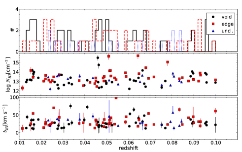
Figure 8: Distribution of observables as a function of redshift. Middle and bottom panels show the distribution of $N_{\rm HI}$ and $b_{\rm HI}$ respectively. Different LSS samples are shown by different color/symbols: void (black circles), void-edge (red squares) and unclassified (blue triangles). Top panel shows the distribution of different LSS as a function of redshift: void (black-solid line), void-edge (red-dashed line) and unclassified (blue-dotted line). For simplicity we only show LSS definitions based on $X$.

A.3 Observables as a function of redshift

We also checked that no bias is present in our samples as a function of redshift. Figure 8 shows both $N_{\rm HI}$ and $b_{\rm HI}$ values as a function of redshift (middle and bottom panels). Systems belonging to different LSS samples are shown by different color/symbols. Both distributions look very uniform across the full redshift range. The top panel shows the distribution of void, void-edge and unclassified absorbers as a function of redshift. The KS test shows no significant difference between these LSS samples. We conclude that there is no evident systematic effect as a function of redshift. For simplicity we have only used LSS definitions based on $X$ in Figure 8, but the previous results also hold using $D$ instead.

The catalog of P12 used a nearly complete, magnitude limited sample of galaxies to define the voids. Despite this, we performed an independent check by looking at the mean radius $\langle R_{\rm void}\rangle$ as a function of redshift. If the catalog is well defined, we should expect to have this radius constant across redshift range (assuming no measurable evolution). We confirmed that this is actually the case by dividing the sample in $6$ redshift bins and measuring the mean value. We found that the mean radius is constant with $\langle R_{\rm void}\rangle\approx 13\pm 3$ $h^{-1}$Mpc in each bin.

References

- Abazajian et al. (2009) Abazajian K. N., Adelman-McCarthy J. K., Agüeros M. A., Allam S. S., Allende Prieto C., An D., Anderson K. S. J., Anderson S. F. et al, 2009, ApJS, 182, 543
- Adelberger et al. (2003) Adelberger K. L., Steidel C. C., Shapley A. E., Pettini M., 2003, ApJ, 584, 45
- Aragón-Calvo et al. (2010) Aragón-Calvo M. A., van de Weygaert R., Jones B. J. T., 2010, MNRAS, 408, 2163
- Baugh et al. (2005) Baugh C. M., Lacey C. G., Frenk C. S., Granato G. L., Silva L., Bressan A., Benson A. J., Cole S., 2005, MNRAS, 356, 1191
- Benson et al. (2003) Benson A. J., Hoyle F., Torres F., Vogeley M. S., 2003, MNRAS, 340, 160
- Bond et al. (1996) Bond J. R., Kofman L., Pogosyan D., 1996, Nature, 380, 603
- Bond et al. (2010) Bond N. A., Strauss M. A., Cen R., 2010, MNRAS, 409, 156
- Borgani et al. (2002) Borgani S., Governato F., Wadsley J., Menci N., Tozzi P., Quinn T., Stadel J., Lake G., 2002, MNRAS, 336, 409
- Bower et al. (2006) Bower R. G., Benson A. J., Malbon R., Helly J. C., Frenk C. S., Baugh C. M., Cole S., Lacey C. G., 2006, MNRAS, 370, 645
- Carswell & Rees (1987) Carswell R. F., Rees M. J., 1987, MNRAS, 224, 13P
- Ceccarelli et al. (2006) Ceccarelli L., Padilla N. D., Valotto C., Lambas D. G., 2006, MNRAS, 373, 1440
- Cen & Ostriker (1999) Cen R., Ostriker J. P., 1999, ApJ, 514, 1
- Chen et al. (1998) Chen H.-W., Lanzetta K. M., Webb J. K., Barcons X., 1998, ApJ, 498, 77
- Chen & Mulchaey (2009) Chen H.-W., Mulchaey J. S., 2009, ApJ, 701, 1219
- Chen et al. (2005) Chen H.-W., Prochaska J. X., Weiner B. J., Mulchaey J. S., Williger G. M., 2005, ApJL, 629, L25
- Colberg et al. (2008) Colberg J. M., Pearce F., Foster C., Platen E., Brunino R., Neyrinck M., Basilakos S., Fairall A. et al, 2008, MNRAS, 387, 933
- Colberg et al. (2005) Colberg J. M., Sheth R. K., Diaferio A., Gao L., Yoshida N., 2005, MNRAS, 360, 216
- Colless et al. (2001) Colless M., Dalton G., Maddox S., Sutherland W., Norberg P., Cole S., Bland-Hawthorn J., Bridges T. et al, 2001, MNRAS, 328, 1039
- Crain et al. (2009) Crain R. A., Theuns T., Dalla Vecchia C., Eke V. R., Frenk C. S., Jenkins A., Kay S. T., Peacock J. A. et al, 2009, MNRAS, 399, 1773
- Crighton et al. (2011) Crighton N. H. M., Bielby R., Shanks T., Infante L., Bornancini C. G., Bouché N., Lambas D. G., Lowenthal J. D. et al, 2011, MNRAS, 414, 28
- Crighton et al. (2010) Crighton N. H. M., Morris S. L., Bechtold J., Crain R. A., Jannuzi B. T., Shone A., Theuns T., 2010, MNRAS, 402, 1273
- Croft et al. (1998) Croft R. A. C., Weinberg D. H., Katz N., Hernquist L., 1998, ApJ, 495, 44
- Dalla Vecchia & Schaye (2008) Dalla Vecchia C., Schaye J., 2008, MNRAS, 387, 1431
- Danforth & Shull (2008) Danforth C. W., Shull J. M., 2008, ApJ, 679, 194
- Danforth et al. (2006) Danforth C. W., Shull J. M., Rosenberg J. L., Stocke J. T., 2006, ApJ, 640, 716
- Davé et al. (1999) Davé R., Hernquist L., Katz N., Weinberg D. H., 1999, ApJ, 511, 521
- Davé et al. (2010) Davé R., Oppenheimer B. D., Katz N., Kollmeier J. A., Weinberg D. H., 2010, MNRAS, 408, 2051
- Doyle et al. (2005) Doyle M. T., Drinkwater M. J., Rohde D. J., Pimbblet K. A., Read M., Meyer M. J., Zwaan M. A., Ryan-Weber E. et al, 2005, MNRAS, 361, 34
- Ferland et al. (1998) Ferland G. J., Korista K. T., Verner D. A., Ferguson J. W., Kingdon J. B., Verner E. M., 1998, PASP, 110, 761
- Fukugita et al. (1998) Fukugita M., Hogan C. J., Peebles P. J. E., 1998, ApJ, 503, 518
- Fukugita & Peebles (2004) Fukugita M., Peebles P. J. E., 2004, ApJ, 616, 643
- Fumagalli et al. (2011) Fumagalli M., Prochaska J. X., Kasen D., Dekel A., Ceverino D., Primack J. R., 2011, MNRAS, 418, 1796
- Gehrels (1986) Gehrels N., 1986, ApJ, 303, 336
- González & Padilla (2010) González R. E., Padilla N. D., 2010, MNRAS, 407, 1449
- Green et al. (2012) Green J. C., Froning C. S., Osterman S., Ebbets D., Heap S. H., Leitherer C., Linsky J. L., Savage B. D. et al, 2012, ApJ, 744, 60
- Gunn & Peterson (1965) Gunn J. E., Peterson B. A., 1965, ApJ, 142, 1633
- Haardt & Madau (1996) Haardt F., Madau P., 1996, ApJ, 461, 20
- Hoyle & Vogeley (2002) Hoyle F., Vogeley M. S., 2002, ApJ, 566, 641
- Hui & Gnedin (1997) Hui L., Gnedin N. Y., 1997, MNRAS, 292, 27
- Icke (1984) Icke V., 1984, MNRAS, 206, 1P
- Kirkman et al. (2007) Kirkman D., Tytler D., Lubin D., Charlton J., 2007, MNRAS, 376, 1227
- Kreckel et al. (2011) Kreckel K., Platen E., Aragón-Calvo M. A., van Gorkom J. H., van de Weygaert R., van der Hulst J. M., Kovač K., Yip C.-W. et al, 2011, AJ, 141, 4
- Lanzetta et al. (1995) Lanzetta K. M., Bowen D. V., Tytler D., Webb J. K., 1995, ApJ, 442, 538
- Lehner et al. (2007) Lehner N., Savage B. D., Richter P., Sembach K. R., Tripp T. M., Wakker B. P., 2007, ApJ, 658, 680
- Lewis et al. (2002) Lewis I., Balogh M., De Propris R., Couch W., Bower R., Offer A., Bland-Hawthorn J., Baldry I. K. et al, 2002, MNRAS, 334, 673
- Lopez et al. (2008) Lopez S., Barrientos L. F., Lira P., Padilla N., Gilbank D. G., Gladders M. D., Maza J., Tejos N. et al, 2008, ApJ, 679, 1144
- Mo & Morris (1994) Mo H. J., Morris S. L., 1994, MNRAS, 269, 52
- Moos et al. (2000) Moos H. W., Cash W. C., Cowie L. L., Davidsen A. F., Dupree A. K., Feldman P. D., Friedman S. D., Green J. C. et al, 2000, ApJL, 538, L1
- Morris & Jannuzi (2006) Morris S. L., Jannuzi B. T., 2006, MNRAS, 367, 1261
- Morris & van den Bergh (1994) Morris S. L., van den Bergh S., 1994, ApJ, 427, 696
- Morris et al. (1993) Morris S. L., Weymann R. J., Dressler A., McCarthy P. J., Smith B. A., Terrile R. J., Giovanelli R., Irwin M., 1993, ApJ, 419, 524
- Padilla et al. (2009) Padilla N., Lacerna I., Lopez S., Barrientos L. F., Lira P., Andrews H., Tejos N., 2009, MNRAS, 395, 1135
- Padilla et al. (2010) Padilla N., Lambas D. G., González R., 2010, MNRAS, 409, 936
- Pan et al. (2012) Pan D. C., Vogeley M. S., Hoyle F., Choi Y.-Y., Park C., 2012, MNRAS, 421, 926
- Park et al. (2007) Park C., Choi Y.-Y., Vogeley M. S., Gott III J. R., Blanton M. R., SDSS Collaboration, 2007, ApJ, 658, 898
- Peebles (2001) Peebles P. J. E., 2001, ApJ, 557, 495
- Penton et al. (2002) Penton S. V., Stocke J. T., Shull J. M., 2002, ApJ, 565, 720
- Prochaska & Tumlinson (2009) Prochaska J. X., Tumlinson J., 2009, Baryons: What,When and Where?, Thronson, H. A., Stiavelli, M., & Tielens, A., ed., p. 419
- Prochaska et al. (2011) Prochaska J. X., Weiner B., Chen H.-W., Mulchaey J., Cooksey K., 2011, ApJ, 740, 91
- Rakic et al. (2011) Rakic O., Schaye J., Steidel C. C., Rudie G. C., 2011, ArXiv e-prints
- Regos & Geller (1991) Regos E., Geller M. J., 1991, ApJ, 377, 14
- Rojas et al. (2005) Rojas R. R., Vogeley M. S., Hoyle F., Brinkmann J., 2005, ApJ, 624, 571
- Rollinde et al. (2003) Rollinde E., Petitjean P., Pichon C., Colombi S., Aracil B., D’Odorico V., Haehnelt M. G., 2003, MNRAS, 341, 1279
- Rudie et al. (2012) Rudie G. C., Steidel C. C., Trainor R. F., Rakic O., Bogosavljevic M., Pettini M., Reddy N., Shapley A. E. et al, 2012, ArXiv e-prints
- Ryan-Weber (2006) Ryan-Weber E. V., 2006, MNRAS, 367, 1251
- Savage & Sembach (1991) Savage B. D., Sembach K. R., 1991, ApJ, 379, 245
- Schaye (2001) Schaye J., 2001, ApJ, 559, 507
- Schaye & Dalla Vecchia (2008) Schaye J., Dalla Vecchia C., 2008, MNRAS, 383, 1210
- Schaye et al. (2010) Schaye J., Dalla Vecchia C., Booth C. M., Wiersma R. P. C., Theuns T., Haas M. R., Bertone S., Duffy A. R. et al, 2010, MNRAS, 402, 1536
- Schaye et al. (1999) Schaye J., Theuns T., Leonard A., Efstathiou G., 1999, MNRAS, 310, 57
- Sheth & van de Weygaert (2004) Sheth R. K., van de Weygaert R., 2004, MNRAS, 350, 517
- Shone et al. (2010) Shone A. M., Morris S. L., Crighton N., Wilman R. J., 2010, MNRAS, 402, 2520
- Shull et al. (2000) Shull J. M., Giroux M. L., Penton S. V., Tumlinson J., Stocke J. T., Jenkins E. B., Moos H. W., Oegerle W. R. et al, 2000, ApJL, 538, L13
- Shull et al. (2011) Shull J. M., Smith B. D., Danforth C. W., 2011, ArXiv e-prints
- Spinrad et al. (1993) Spinrad H., Filippenko A. V., Yee H. K., Ellingson E., Blades J. C., Bahcall J. N., Jannuzi B. T., Bechtold J. et al, 1993, AJ, 106, 1
- Springel et al. (2005) Springel V., White S. D. M., Jenkins A., Frenk C. S., Yoshida N., Gao L., Navarro J., Thacker R. et al, 2005, Nature, 435, 629
- Stinson et al. (2011) Stinson G., Brook C., Prochaska J. X., Hennawi J., Pontzen A., Shen S., Wadsley J., Couchman H. et al, 2011, ArXiv e-prints
- Stocke et al. (2007) Stocke J. T., Danforth C. W., Shull J. M., Penton S. V., Giroux M. L., 2007, ApJ, 671, 146
- Stocke et al. (2006) Stocke J. T., Penton S. V., Danforth C. W., Shull J. M., Tumlinson J., McLin K. M., 2006, ApJ, 641, 217
- Stocke et al. (1995) Stocke J. T., Shull J. M., Penton S., Donahue M., Carilli C., 1995, ApJ, 451, 24
- Tepper-García et al. (2012) Tepper-García T., Richter P., Schaye J., Booth C. M., Dalla Vecchia C., Theuns T., 2012, ArXiv e-prints
- Theuns et al. (1998a) Theuns T., Leonard A., Efstathiou G., 1998a, MNRAS, 297, L49
- Theuns et al. (1998b) Theuns T., Leonard A., Efstathiou G., Pearce F. R., Thomas P. A., 1998b, MNRAS, 301, 478
- Theuns et al. (1999) Theuns T., Leonard A., Schaye J., Efstathiou G., 1999, MNRAS, 303, L58
- Theuns et al. (2002) Theuns T., Viel M., Kay S., Schaye J., Carswell R. F., Tzanavaris P., 2002, ApJL, 578, L5
- Tikhonov & Klypin (2009) Tikhonov A. V., Klypin A., 2009, MNRAS, 395, 1915
- Tilton et al. (2012) Tilton E. M., Danforth C. W., Shull J. M., Ross T. L., 2012, ArXiv e-prints
- van de Weygaert & van Kampen (1993) van de Weygaert R., van Kampen E., 1993, MNRAS, 263, 481
- Wakker & Savage (2009) Wakker B. P., Savage B. D., 2009, ApJS, 182, 378
- Wiersma et al. (2009a) Wiersma R. P. C., Schaye J., Smith B. D., 2009a, MNRAS, 393, 99
- Wiersma et al. (2009b) Wiersma R. P. C., Schaye J., Theuns T., Dalla Vecchia C., Tornatore L., 2009b, MNRAS, 399, 574
- Williger et al. (2000) Williger G. M., Smette A., Hazard C., Baldwin J. A., McMahon R. G., 2000, ApJ, 532, 77
- Wilman et al. (2007) Wilman R. J., Morris S. L., Jannuzi B. T., Davé R., Shone A. M., 2007, MNRAS, 375, 735
- Woodgate et al. (1998) Woodgate B. E., Kimble R. A., Bowers C. W., Kraemer S., Kaiser M. E., Danks A. C., Grady J. F., Loiacono J. J. et al, 1998, PASP, 110, 1183