Photoinduced reordering in thin azo-dye films and light-induced reorientation dynamics of nematic liquid-crystal easy axis

Abstract

We theoretically study the kinetics of photoinduced reordering triggered by linearly polarized (LP) reorienting light in thin azo-dye films that were initially illuminated with LP ultraviolet (UV) pumping beam. The process of reordering is treated as a rotational diffusion of molecules in the light intensity-dependent mean-field potential. The two dimensional (2D) diffusion model which is based on the free energy rotational Fokker-Planck equation and describes the regime of in-plane reorientation is generalized to analyze the dynamics of the azo-dye order parameter tensor at varying polarization azimuth of the reorienting light. It is found that, in the photosteady state, the intensity of LP reorienting light determines the scalar order parameter (the largest eigenvalue of the order parameter tensor), whereas the steady state orientation of the corresponding eigenvector (the in-plane principal axis) depends solely on the polarization azimuth. We show that, under certain conditions, reorientation takes place only if the reorienting light intensity exceeds its critical value. Such threshold behavior is predicted to occur in the bistability region provided that the initial principal axis lies in the polarization plane of reorienting light. The model is used to interpret the experimental data on the light-induced azimuthal gliding of liquid-crystal easy axis on photoaligned azo-dye substrates.

I Introduction

Linearly polarized (LP) ultraviolet (UV) or visible light is known to have a profound effect on the physical properties of some photosensitive materials such as compounds containing azobenzene and its derivatives Zhao and Ikeda (2009). In particular, such materials may become dichroic and birefringent under the action of LPUV light. Over the past few decades this phenomenon — the so-called effect of photoinduced optical anisotropy (POA) — which has a long history dating back almost a century to the original paper by Weigert Weigert (1919) has been attracted much attention for both technological and fundamental reasons. POA is of primary importance in the development of tools dealing with the light-controlled anisotropy and the materials that exhibit POA are very promising for use in many photonic applications Eich et al. (1987); Natansohn et al. (1992); Prasad et al. (1995); Blinov et al. (1999).

POA also lies at the heart of the photoalignment (PA) technique which is employed in the manufacturing process of liquid crystal displays for fabricating high quality aligning substrates Yang and Wu (2006); Chigrinov et al. (2008). This method avoids the drawbacks of the traditional mechanical surface treatment and uses LPUV light to induce anisotropy of the angular distribution of molecules in a photosensitive film O’Neill and Kelly (2000); Chigrinov et al. (2008).

When the irradiated layer is brought in contact with a liquid crystal (LC), the surface ordering originated from the photoinduced anisotropy manifests itself in the anisotropic part of the surface tension known as the anchoring energy and determines the anchoring characteristics such as the anchoring strengths and the easy axis, $\mathbf{n}_{e}$, that defines the direction of preferential orientation of LC molecules at the surface. In this way, the light can be used as a means to control the anchoring properties of photosensitive materials.

This is the light-induced anisotropy of the orientational distribution of molecules that reveals itself in POA and can be described as the photoinduced orientational ordering in photosensitive materials. Such ordering, though not being understood very well, can generally occur by a variety of photochemically induced processes. These typically may involve such transformations as photoisomerization, crosslinking, photodimerization and photodecomposition (a recent review can be found in Refs. Chigrinov et al. (2003a, 2008)).

The mechanism of photoinduced ordering underlying POA and related photoaligning properties therefore cannot be universal. Rather they crucially depend on the material in question and on a number of additional factors such as irradiation conditions, surface interactions etc. These factors combined with the action of light may result in different regimes of the photoinduced ordering kinetics leading to the formation of various photoinduced orientational structures.

The photoalignment has been studied in a number of polymer systems including dye doped polymer layers Gibbons et al. (1991); Furumi et al. (1999), cinnamate polymer derivatives Schadt et al. (1992); Dyadyusha et al. (1992); Galabova et al. (1996); Perny et al. (2000) and side chain polymers containing chemically linked azochromophores (azopolymers) Petry et al. (1993); Holme et al. (1996); Blinov et al. (1998); Wu et al. (2000). POA observed in similar polymers Eich et al. (1987); Natansohn et al. (1992); Holme et al. (1996); Petry et al. (1993); Wiesner et al. (1992); Blinov et al. (1998); Yaroshchuk et al. (2001) was found to be long term stable so that the photoinduced anisotropy does not disappear after switching off the irradiation.

Most of the above mentioned polymer systems represent azocompounds that exhibit POA driven by the trans-cis photoisomerization. In theoretical models Pedersen and Johansen (1997); Pedersen et al. (1998); Puchkovs’ka et al. (1998); Sajti et al. (2001); Yaroshchuk et al. (2001); Kiselev (2002); Sekkat et al. (2002), they are treated as ensembles of the stable trans isomers characterized by elongated rod-like molecular conformation and the bent banana-like shaped cis isomers.

The mechanism of photoisomerization implies that the key processes behind the photoinduced orientational ordering of azo-dye molecules are photochemically induced trans-cis  isomerization and subsequent thermal and/or photochemical cis-trans  back isomerization of azobenzene chromophores. Owing to pronounced absorption dichroism of photoactive groups, the photoisomerization rate strongly depends on orientation of the azo-dye molecules relative to the polarization vector of the pumping light, $\mathbf{E}_{UV}$.

When the cis isomers are short-living, the cis state becomes temporary populated during photoisomerization but reacts immediately back to the stable trans isomeric form. The trans-cis-trans isomerization cycles are accompanied by rotations of the azo-dye molecules that tend to minimize the absorption and become oriented along directions normal to the polarization vector of the exciting light $\mathbf{E}_{UV}$ (the molecules with the optical transition dipole moment oriented perpendicular to $\mathbf{E}_{UV}$ are almost inactive). Non-photoactive groups may then undergo reorientation due to cooperative motion Holme et al. (1996); Natansohn et al. (1998); Puchkovs’ka et al. (1998); Kiselev (2002); Sekkat et al. (2002).

From the above it might be concluded that the photoinduced orientational structures will be uniaxially anisotropic with the optical axis directed along the polarization vector, $\mathbf{E}_{UV}$. Experimentally, this is, however, not the case. For example, constraints imposed by a medium may suppress out-of-plane reorientation of the azobenzene chromophores giving rise to the structures with strongly preferred in-plane alignment Yaroshchuk et al. (2001). Another symmetry breaking effect induced by polymeric environment is that the photoinduced orientational structures can be biaxial Wiesner et al. (1992); Buffeteau and Pézolet (1998); Kiselev et al. (2001); Yaroshchuk et al. (2001); Kiselev (2002); Yaroshchuk et al. (2003) (a recent review of medium effects on photochemical processes can be found in Kaanumalle et al. (2005)).

It was recently found that, similar to the polymer systems, the long-term stable POA in the films containing photochemically stable azo-dye structures (azobenzene sulfuric dyes) is characterized by the biaxial photoinduced structures with favored in-plane alignment Kiselev et al. (2008, 2009). Unlike azopolymers, photochromism in these films is extremely weak so that it is very difficult to unambiguously detect the presence of a noticeable fraction of cis isomers.

Over the last decade the photoaligning properties of such azo-dye (SD1) films has been the subject of intense studies Chigrinov et al. (2008, 2002, 2003b); Kiselev et al. (2005). It was found that, owing to high degree of the photoinduced ordering, these films used as aligning substrates are characterized by the anchoring energy strengths comparable to the rubbed polyimide films. For these materials, the voltage holding ratio and thermal stability of the alignment turned out to be high. The azo-dye films are thus promising materials for applications in liquid crystal devices.

The anchoring characteristics of the azo-dye films such as the polar and azimuthal anchoring energies are strongly influenced by the photoinduced ordering. In particular, the easy axis is dictated by the polarization of the pumping LPUV light, whereas the azimuthal and polar anchoring strengths may depend on a number of the governing parameters such as the wavelength and the irradiation dose Kiselev et al. (2005).

In a LC cell with the initially irradiated layer, the easy axis may rotate under the action of secondary irradiation with reorienting LP light which polarization differs from the one used to prepare the aligning layer. This effect — the so-called light-induced reorientation of the easy axis — is governed by the photoinduced reordering of azo-dye molecules triggered by the reorienting light and may be of considerable interest for applications such as LC rewritable devices Muravsky et al. (2008). Note that slow reorientation of the easy axis (the light-induced easy axis gliding) on the photosensitive layers prepared using the PA technique was originally observed on poly-(vinyl)-alcohol (PVA) coatings with embedded azo-dye molecules Vorflusev et al. (1997). For the azo-dye films, similar results were reported in Ref. Pasechnik et al. (2006).

In this paper the kinetics of photoinduced reordering underlying the light-induced easy axis reorientation on the azo-dye films will be our primary concern. In particular, we apply a generalized version of the theoretical analysis presented in Ref. Kiselev et al. (2009) to examine how the initial ordering of azo-dye molecules and the characteristics of reorienting light affect the regime of kinetics and the photosteady states.

There are two phenomenological models formulated in Ref. Kiselev et al. (2009) by using different theoretical approaches: (a) the two-state model is based on the above discussed mechanism of photoisomerization with short living excited cis state which is characterized by weak photochromism and negligibly small fraction of cis molecules that rapidly decays after switching off irradiation; and (b) the diffusion model describes the light-induced reorientation of azo-dye molecules as rotational Brownian motion governed by the light intensity-dependent mean-field potential. It turned out that predictions of the models are quite similar and they both were successfully used to interpret the experimental data. This equivalence points to the fact that, in the limiting case of short-living cis states, the photoisomerization cycles with orientation dependent isomerization rates may generally be viewed as a random walk on the sphere described by the Fokker-Planck equation for rotational diffusion. For our purposes, the latter will be conveniently employed to perform the theoretical analysis and to model the kinetics of reordering.

The layout of the paper is as follows. In Sec. II we briefly recapitulate the theory Kiselev et al. (2009) introducing the diffusion models where the process of photoinduced reordering is treated as a rotational diffusion in the effective mean-field potential. Then, in Sec. II.2, we discuss the regime of purely in-plane reorientation and analyze the general properties of the corresponding two dimensional (2D) diffusion model. In Sec. III these results are used to study bifurcations of the photosteady states and the kinetics of photoinduced reordering depending on the initial ordering, the light intensity, $I_{UV}$ and the polarization azimuth, $\alpha_{p}$, that characterizes orientation of the polarization vector of reorienting LPUV light, $\mathbf{E}_{UV}$. In Sec. IV we apply the model to interpret the experimental data on the light-induced azimuthal gliding of the easy axis on the photoaligned SD1 substrate measured as part of the investigation into effects of the polarization azimuth in the dynamics of the electrically assisted light-induced gliding Dubtsov et al. (2012). Finally, in Sec. V we draw the results together and make some concluding remarks.

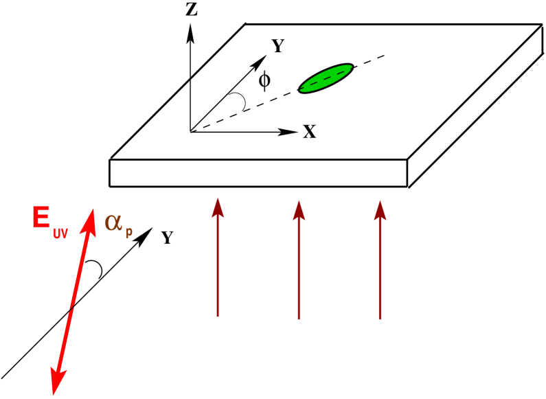
Figure 1: (Color online) Frame of reference: the $z$ axis is normal to the substrate and the polarization vector of the activating light makes the angle $\alpha_{p}$ with the $y$ axis.

II Model

In this section our starting point is the approach of Ref. Kiselev et al. (2009) in which the light-induced reorientation of azo-dye molecules is described as rotational Brownian motion governed by the effective mean-field potential.

Following Ref. Kiselev et al. (2009), we assume that azo-dye molecules are cylindrically symmetric, so that orientation of a molecule can be specified by the unit vector, $\hat{\mathbf{u}}=(\sin\theta\cos\phi,\sin\theta\sin\phi,\cos\theta)$, directed along the long molecular axis. Quadrupolar orientational ordering of such molecules is characterized using the traceless symmetric second-rank tensor de Gennes and Prost (1993)

$$\mathbf{Q}(\hat{\mathbf{u}})=(3\,\hat{\mathbf{u}}\otimes\hat{\mathbf{u}}-\mathbf{I}_{3})/2,$$ (1)

where $\mathbf{I}_{n}$ is the $n\times n$ identity matrix. The dyadic (1) can be averaged over orientation of molecules with the normalized angular distribution function $f(\hat{\mathbf{u}},t)$ to yield the order parameter tensor $\mathbf{S}$

$$\langle{\mathbf{Q}}\rangle=\int\mathbf{Q}(\hat{\mathbf{u}})f(\hat{\mathbf{u}},t)\,\mathrm{d}\hat{\mathbf{u}}=\mathbf{S},$$ (2)

where $\mathrm{d}\hat{\mathbf{u}}\equiv\sin\theta\mathrm{d}\theta\mathrm{d}\phi$.

II.1 Rotational mean-field Fokker-Planck equation

The key assumption taken in the diffusion models formulated in Ref. Kiselev et al. (2009) is that the angular distribution function, $f(\hat{\mathbf{u}},t)$, of rodlike azo-dye molecules must satisfy the rotational free energy Fokker-Planck (FP) equation

$$\partial_{t}f=-\mathcal{L}_{i}D_{ij}^{(\mathrm{rot})}\left\{f\,\mathcal{L}_{j}\,\dfrac{\delta F[f]}{\delta f}\right\}\equiv-\mathbf{L}\cdot\mathbf{D}_{\mathrm{rot}}\left\{f\cdot\mathbf{L}\,\dfrac{\delta F[f]}{\delta f}\right\},$$ (3)

where $D_{ij}^{(\mathrm{rot})}$ is the rotational diffusion tensor and $\mathbf{L}$ is the angular momentum operator that can be expressed in terms of of the azimuthal and zenithal (polar) angles, $\phi$ and $\theta$, as follows

$$i\,\mathbf{L}=[\mathbf{r}\times\boldsymbol{\nabla}]=\hat{\mathbf{e}}_{\phi}\,\partial_{\theta}-[\sin\theta]^{-1}\hat{\mathbf{e}}_{\theta}\,\partial_{\phi},$$ (4)

where $\hat{\mathbf{e}}_{\theta}=(\cos\theta\,\cos\phi,\cos\theta\,\sin\phi,-\sin\theta)$ and $\hat{\mathbf{e}}_{\phi}=(-\sin\phi,\cos\phi,0)$.

When the effective free energy functional is a sum of the effective internal energy, $U[f]$, and the Boltzmann entropy, $\langle{\ln f}\rangle$, $F[f]=U[f]+\langle{\ln f}\rangle$, the free energy FP  (3) can be recast into the form of the mean-field FP equation

$$\partial_{t}f=-\mathbf{L}\cdot\mathbf{D}_{\mathrm{rot}}\left\{\mathbf{L}\,f+f\cdot\mathbf{L}\,V\right\},\quad V=\dfrac{\delta U}{\delta f}.$$ (5)

describing the rotational diffusion governed by the effective mean-field potential, $V$.

II.1.1 Effective mean-field potential

In the lowest order approximation based on the truncated expansion for the internal energy functional $U[f]$ retaining one-particle (linear) and two-particle (quadratic) terms, the effective potential, $V$, is given by

$$V(\hat{\mathbf{u}})=\dfrac{\delta U}{\delta f(\hat{\mathbf{u}})}=U_{1}(\hat{\mathbf{u}})+\int U_{2}(\hat{\mathbf{u}},\hat{\mathbf{u}}^{\,\prime})f(\hat{\mathbf{u}}^{\,\prime})\,\mathrm{d}\hat{\mathbf{u}}^{\,\prime},$$ (6)

where $U_{1}(\hat{\mathbf{u}})$ is the external field potential and the last term proportional to the symmetrized two-particle kernel, $U_{2}(\hat{\mathbf{u}},\hat{\mathbf{u}}^{\,\prime})$, represents the contribution coming from the intermolecular interactions.

The one-particle part of the effective potential (6) can be written as a sum of the light-induced contribution

$$U_{I}(\hat{\mathbf{u}})=u_{I}\,{\mathbf{E}}^{\ast}_{UV}\cdot\mathbf{Q}(\hat{\mathbf{u}})\cdot\mathbf{E}_{UV},$$ (7)

where an asterisk indicates complex conjugation, that comes from the interaction of azo-molecules with the reorienting UV light and the surface-induced potential

$$U_{s}(\hat{\mathbf{u}})=u_{s}\,\hat{\mathbf{z}}\cdot\mathbf{Q}(\hat{\mathbf{u}})\cdot\hat{\mathbf{z}}=u_{s}\,Q_{zz}(\hat{\mathbf{u}})$$ (8)

that takes into account conditions at the bounding surfaces of the azo-dye layer. So, for the two-particle interaction taken in the Maier-Saupe form

$$U_{2}(\hat{\mathbf{u}}_{1},\hat{\mathbf{u}}_{2})=u_{2}\,\mathop{\rm Tr}\nolimits[\mathbf{Q}(\hat{\mathbf{u}}_{1})\cdot\mathbf{Q}(\hat{\mathbf{u}}_{2})]=u_{2}\,Q_{ij}(\hat{\mathbf{u}}_{1})Q_{ij}(\hat{\mathbf{u}}_{2}),$$ (9)

we obtain the following expression for the effective potential of azo-dye molecules:

$$V(\hat{\mathbf{u}})=u_{I}I_{UV}\,\hat{\mathbf{e}}_{p}\cdot\mathbf{Q}(\hat{\mathbf{u}})\cdot\hat{\mathbf{e}}_{p}+u_{s}\,Q_{zz}(\hat{\mathbf{u}})+u_{2}S_{ij}\,Q_{ij}(\hat{\mathbf{u}}),$$ (10)

where $I_{UV}$ is the intensity of the reorienting UV light which is assumed to be linearly polarized along the unit polarization vector $\hat{\mathbf{e}}_{p}$

$$\hat{\mathbf{e}}_{p}=\mathbf{R}_{\mathrm{rot}}(\alpha_{p})\,\hat{\mathbf{y}},\quad\mathbf{R}_{\mathrm{rot}}(\alpha_{p})=\begin{pmatrix}\cos\alpha_{p}&-\sin\alpha_{p}\\ \sin\alpha_{p}&\cos\alpha_{p}\end{pmatrix}$$ (11)

that makes the angle $\alpha_{p}$ with the $y$ axis directed along the polarization vector of the initial irradiation: $\mathbf{E}_{\mathrm{ini}}\parallel\hat{\mathbf{y}}$ (see Fig. 1).

Note that, in the limiting case of non-interacting molecules with $U_{2}=0$, the rotational mean-field FP equation (5) reduces to the well-known linear rotational diffusion equation that has been widely used to study a large variety of problems based on the rotational diffusion model for the rotational motion of molecules in the presence of external fields. These include dielectric and Kerr effect relaxation of polar liquids Lauritzen and Zwanzig (1973); Coffey et al. (1993); Dejárdin et al. (1993); Dejárdin and Kalmykov (2000); Kalmykov and Quinn (1991); Felderhof (2002); Kalmykov (2001); Kalmykov and Titov (2007), rotational diffusion of a probe molecule dissolved in a liquid crystal phase Nordio and Busolin (1971); Tarroni and Zannoni (1991); Luckhurst and Sanson (1972); Berggren et al. (1993); Ferrarini et al. (1994); Brognara et al. (2000) and the molecular reorientation in liquid crystal phases Nordio and Serge (1979); Moro and Nordio (1984); Dozov et al. (1987); Fontana et al. (1986).

II.1.2 Steady states

The equilibrium angular distribution can generally be obtained as a stationary solution to the FP equation (5). It can be readily checked that the Boltzmann distribution

$$f_{\,\mathrm{st}}(\hat{\mathbf{u}})=Z_{\,\mathrm{st}}^{-1}\,\exp[-V(\hat{\mathbf{u}})],\quad Z_{\mathrm{st}}=\int\exp[-V(\hat{\mathbf{u}})]\mathrm{d}\hat{\mathbf{u}}$$ (12)

determined by the effective potential gives the stationary solution. Note that the energy scale is determined by the temperature factor $k_{B}T$ incorporated into the rotation diffusion tensor, so that the internal energy, $U[f]$, and the potential, $V$, are both dimensionless.

When the FP equation is linear, the stationary distribution (12) describing the equilibrium state is unique. By contrast, this is no longer the case when the effective potential (10) depends on the elements of the averaged orientational order parameter tensor (2): $V(\hat{\mathbf{u}})=V(\hat{\mathbf{u}}|\mathbf{S})$. In this case, the components of the order parameter tensor in the stationary state, $S_{ij}=S_{ij}^{(\mathrm{st})}$, can be found from the self-consistency equation

$$S_{ij}=\int Q_{ij}(\hat{\mathbf{u}})\,f_{\,\mathrm{st}}(\hat{\mathbf{u}}|\mathbf{S})\,\mathrm{d}\hat{\mathbf{u}}.$$ (13)

which generally possesses several solutions representing multiple local extrema (stationary points) of the free energy

$$F[f_{\,\mathrm{st}}]\equiv F_{\,\mathrm{st}}(\mathbf{S})=-\frac{u_{2}}{2}\,S_{ij}S_{ij}-\ln Z_{\,\mathrm{st}}(\mathbf{S}).$$ (14)

Following the line of reasoning presented in Ref. Frank (2005) and using the effective free energy as the Lyapunov functional, it is not difficult to prove the $H$ theorem for nonlinear FP equations of the form (3). It follows that, in the long time limit, all transient solutions converge to stationary ones. So, each stable stationary distribution is characterized by the basin of attraction giving orientational states (angular distributions) that evolve in time approaching the stationary distribution.

II.2 Two-dimensional model of purely in-plane reorientation

In the previous section our model has been formulated as the free energy FP equation (5) describing rotational diffusion of azo-dye molecules governed by the effective mean field potential (10). In this section, we concentrate on the limiting case of purely in-plane reorientation and deal with the simplified two-dimensional model

$$\partial_{\tau}f= \partial_{\phi}\Bigl{[}\partial_{\phi}f+f\partial_{\phi}V\Bigr{]}=\partial_{\phi}^{2}f+\frac{1}{2}\,\Bigl{[}\,\partial_{\phi}^{2}(fV)$$

$$+f\partial_{\phi}^{2}V-V\partial_{\phi}^{2}f\Bigr{]},\quad\tau=D_{z}^{(\mathrm{rot})}t.$$ (15)

can be derived by assuming that the out-of-plane component of the unit vector $\hat{\mathbf{u}}$ describing orientation of the azo-dye molecules is suppressed and, as is shown in Fig. 1, $\hat{\mathbf{u}}=(\sin\phi,\cos\phi,0)$. It implies that, similar to the model of a single axis rotator with two equivalent sites Lauritzen and Zwanzig (1973); Coffey et al. (1993), the molecules are constrained to be parallel to the substrate plane (the $x$-$y$ plane).

II.2.1 Potential

When the out-of-plane reorientation is completely suppressed and $\hat{\mathbf{u}}=(\sin\phi,\cos\phi,0)$, the order parameter dyadic (1) simplifies as follows

$$\mathbf{Q}(\phi)=\begin{pmatrix}\mathbf{Q}_{2}(\phi)&\mathbf{0}\\ \mathbf{0}&-1/2\end{pmatrix}$$ (16)

where $\mathbf{Q}_{2}$ is the two-dimensional in-plane part of the tensor. The in-plane order parameter tensor is given by the $2\times 2$ block-matrix

$$4\mathbf{Q}_{2}(\phi)=\mathbf{I}_{2}-3\cos(2\phi)\,\boldsymbol{\sigma}_{3}+3\sin(2\phi)\,\boldsymbol{\sigma}_{1}$$ (17)

expressed in terms of the Pauli matrices: $\boldsymbol{\sigma}_{3}=\begin{pmatrix}1&0\\ 0&-1\end{pmatrix}$ and $\boldsymbol{\sigma}_{1}=\begin{pmatrix}0&1\\ 1&0\end{pmatrix}$. We can now substitute the expression for the order parameter tensor (16) into the effective potential (10) and use the algebraic identity

$$\mathbf{R}_{\mathrm{rot}}(-\alpha)\mathbf{Q}_{2}(\phi)\mathbf{R}_{\mathrm{rot}}(\alpha)=\mathbf{Q}_{2}(\phi+\alpha)$$ (18)

to derive the angular dependent part of the potential in the following form:

$$V=\bigl{(}{v}^{\ast}\exp[2i\phi]+v\exp[-2i\phi]\bigr{)}/2,$$ (19a)

$$v=v_{1}\exp[-2i\alpha_{p}]+v_{2}\langle{\exp[2i\phi]}\rangle,$$ (19b)

$$v_{1}\equiv 3u_{I}I_{UV}/4,\quad v_{2}=9u_{2}/8,$$ (19c)

where $\displaystyle\langle{\ldots}\rangle=\int_{0}^{2\pi}\ldots f\mathrm{d}\phi$; $v_{1}$ and $v_{2}$ are the photoexcitation and intermolecular interaction parameters, respectively.

II.2.2 Fourier harmonics and order parameters

Our next step is to obtain the system of equations for the averaged complex harmonics, $h_{n}(\tau)=\langle{\exp[in\phi]}\rangle(\tau)$, that are proportional to the Fourier coefficients of the distribution function, $f(\phi,\tau)$

$$f(\phi,\tau)=(2\pi)^{-1}\sum_{n=-\infty}^{\infty}h_{n}(\tau)\exp[-in\phi].$$ (20)

To this end, we integrate the FP equation (15) multiplied by $\exp[in\phi]$ over the azimuthal angle. The resulting system reads

$$\partial_{\tau}h_{n}(\tau)=-n^{2}h_{n}+n\,\bigl{\{}{v}^{\ast}(\alpha_{p},h_{2})h_{n+2}(\tau)-v(\alpha_{p},h_{2})h_{n-2}(\tau)\bigr{\}},$$ (21)

where $v(\alpha_{p},h_{2})\equiv v=v_{1}\exp[-2i\alpha_{p}]+v_{2}h_{2}$.

When $f(\phi+\pi)=f(\phi)$, the odd numbered harmonics vanish, $h_{2k+1}=0$. For the even numbered harmonics, $\rho_{k}\equiv h_{2k}$, the system (21) can be conveniently recast into the form

$$\partial_{\tau}\rho_{k}=-4k^{2}\rho_{k}+2k\,({v}^{\ast}\rho_{k+1}-v\rho_{k-1}),\quad k=1,2,\ldots$$ (22)

$$\rho_{k}=p_{k}+iq_{k}=\langle{\cos(2k\phi)}\rangle+i\langle{\sin(2k\phi)}\rangle\equiv h_{2k},\quad\rho_{0}=1,$$ (23)

where $\rho_{1}=p_{1}+iq_{1}=\langle{\exp[2i\phi]}\rangle$ is the complex order parameter harmonics.

For the in-plane order parameter tensor (17) averaged over the azimuthal angle

$$\langle{\mathbf{Q}_{2}}\rangle=\mathbf{S}_{2}=\frac{1}{4}\begin{pmatrix}1-3p_{1}&q_{1}\\ q_{1}&1+3p_{1}\end{pmatrix}=\mathbf{R}_{\mathrm{rot}}(\alpha_{e})\begin{pmatrix}s_{+}&0\\ 0&s_{-}\end{pmatrix}\mathbf{R}_{\mathrm{rot}}(-\alpha_{e}),$$ (24)

$$s_{\pm}=(1\pm 3|\rho_{1}|)/4,\quad 2\alpha_{e}=\arg(-{\rho_{1}}^{\ast}),$$ (25)

the order parameter harmonics, $\rho_{1}$, defines the principal values (eigenvalues), $s_{+}$ and $s_{-}$, and the eigenvector, $(\cos\alpha_{e},\sin\alpha_{e})$, for the largest eigenvalue $s_{+}$ giving the in-plane principal axis: $\hat{\mathbf{n}}_{e}=(\cos\alpha_{e},\sin\alpha_{e},0)$. So, the tensor (24) can be rewritten in the form of the in-plane order parameter dyadic:

$$\mathbf{S}_{2}=s_{-}\mathbf{I}_{2}+(s_{+}-s_{-})\hat{\mathbf{n}}_{e}\otimes\hat{\mathbf{n}}_{e}.$$ (26)

Temporal evolution of the in-plane order parameter tensor is determined by the order parameter harmonics, $\rho_{1}(t)$, that can be computed as a function of time by solving the initial value problem for the system (22) with the initial values of the harmonics $\rho_{k}(0)=\rho_{k}^{(\mathrm{ini})}$ representing the initial angular distribution $f(\phi,0)=f_{\mathrm{ini}}(\phi)$.

II.2.3 Symmetry

It is not difficult to check that the system (21) is invariant under the symmetry transformation

$$h_{n}\to\tilde{h}_{n}=\exp[in\alpha]h_{n},\quad v\to\tilde{v}=\exp[2i\alpha]v=v(\alpha_{p}-\alpha,\tilde{h}_{2}).$$ (27)

An important consequence of these relations concerns the special case where the reorienting light is switched off and $v_{1}=0$. It can be readily seen that, at $v=v_{2}\rho_{1}$, a set of the harmonics, $\{\rho_{k}\}_{k}$, and that of the transformed harmonics $\{\exp[2ik\alpha]\rho_{k}\}_{k}$ both satisfy the system of equations (22). In particular, at $I_{UV}=0$, the stationary angular distribution, $f_{\mathrm{st}}(\phi)$, and the shifted (rotated) one, $f_{\mathrm{st}}(\phi-\alpha)$, both represent steady states.

By using the symmetry relations (27) dynamical equations (22) can be conveniently changed into the system with the zero polarization azimuth, $\alpha_{p}=0$. More precisely, from Eq. (27), it follows that the transformed harmonics

$$\tilde{\rho}_{k}=\exp[2ik\alpha_{p}]\rho_{k}$$ (28)

satisfy the system (22) with the coupling coefficient $v(\alpha_{p},\rho)$ and the initial distribution $f_{\mathrm{ini}}(\phi)$ replaced by $\tilde{v}=v(0,\tilde{\rho}_{1})$ and $\tilde{f}_{\mathrm{ini}}=f_{\mathrm{ini}}(\phi-\alpha_{p})$, respectively. Geometrically, such transformation can be described as a transition to the frame of reference where the $y$ axis is directed along the polarization vector of reorienting light.

So, in the subsequent section, we shall restrict our considerations to the special case of the system with the coupling coefficient

$$\tilde{v}=v_{1}+v_{2}\tilde{\rho}_{1}$$ (29)

taken at $\alpha_{p}=0$. In this case, the polarization azimuth, $\alpha_{p}$, enters the initial data, $\tilde{\rho}_{k}^{(\mathrm{ini})}=\exp[2ik\alpha_{p}]\rho_{k}^{(\mathrm{ini})}$, and the formula

$$\alpha_{e}=\alpha_{p}+\frac{1}{2}\arg(-{\tilde{\rho}_{1}}^{\ast})$$ (30)

gives the azimuthal angle of the principal axis (25) expressed in terms of the order parameter harmonics $\tilde{\rho}_{1}$.

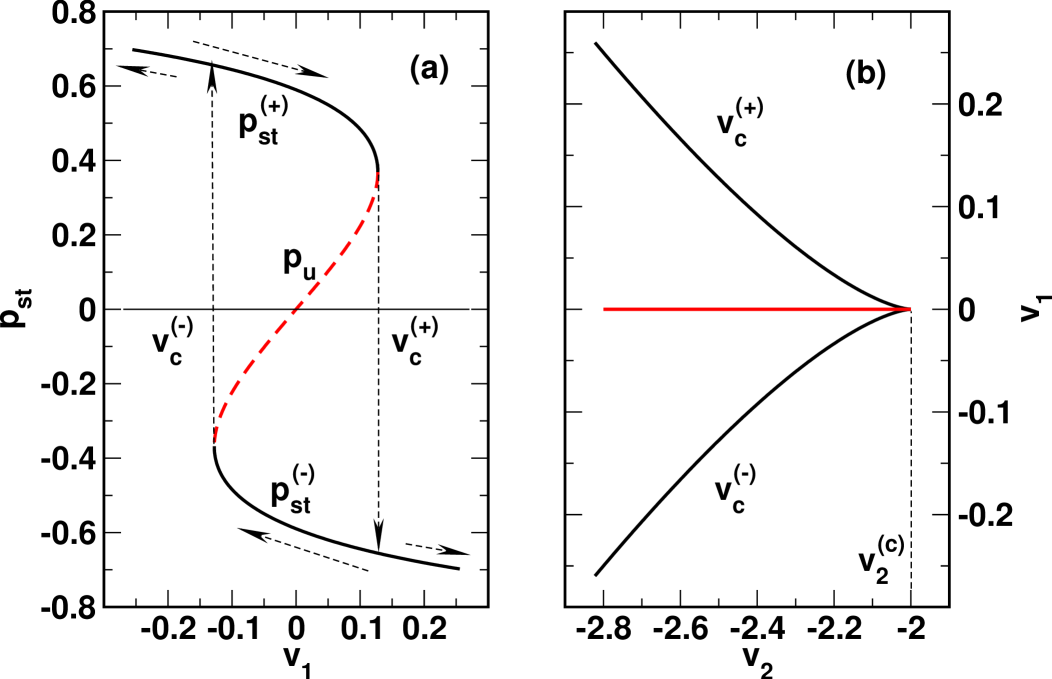
Figure 2: (Color online) (a) Steady state order parameter harmonics $p_{\mathrm{st}}$ as a function of the photoexcitation parameter $v_{1}$ at $v_{2}=-2.5$; (b) bifurcation curves in the $v_{2}$-$v_{1}$ plane are typical of the cusp catastrophe with the cusp singularity located at $(-2,0)$.

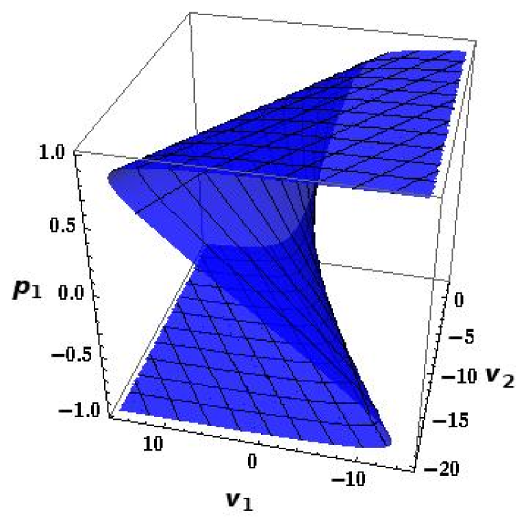
Figure 3: (Color online) Bifurcation diagram as the cusp surface in the three dimensional $(v_{1},v_{2},p_{1})$ space.

III Kinetics of photoinduced in-plane reordering

III.1 Bifurcations of equilibria

The expression for the stationary distributions

$$f_{\mathrm{st}}=Z_{\mathrm{st}}^{-1}\exp[-V]=Z_{\mathrm{st}}^{-1}\exp[-|\tilde{v}|\cos(2\phi-\tilde{\alpha})],\quad Z_{\mathrm{st}}=\int_{0}^{2\pi}\exp[-V]\mathrm{d}\phi$$ (31)

comes from the general formula (12) and represents the photosteady states in the two dimensional case with the potential given in Eq. (19) where the coupling coefficient is changed from $v$ to $\tilde{v}=|\tilde{v}|\exp[i\tilde{\alpha}]$.

Equation (31) can now be combined with the relation

$$\exp[-v\cos 2\phi]=I_{0}(v)+2\sum_{k=1}^{\infty}(-1)^{k}I_{k}(v)\cos 2k\phi,$$ (32)

where $I_{k}$ is the modified Bessel function of integer order Abramowitz and Stegun (1972), to derive the stationary state statistical integral

$$Z_{\mathrm{st}}=2\pi I_{0}(|\tilde{v}|)$$ (33)

and the stationary state free energy (14)

$$F_{\mathrm{st}}(\tilde{v})=v_{2}^{-1}\Bigl{[}-\frac{|\tilde{v}|^{2}}{2}+v_{1}|\tilde{v}|\cos\tilde{\alpha}\Bigr{]}-\ln I_{0}(|\tilde{v}|),$$ (34)

where the additive constant is chosen so as to have the free energy vanishing at $\tilde{v}=0$.

The stationary points of the energy (34), $\tilde{v}=\tilde{v}_{\mathrm{st}}=v_{1}+v_{2}\tilde{\rho}_{1}^{(\mathrm{st})}$, define the steady state distributions (31) characterized by the stationary values of the order parameter harmonics, $\tilde{\rho}_{1}^{(\mathrm{st})}=\tilde{p}_{1}^{(st)}+i\tilde{q}_{1}^{(\mathrm{st})}$, which can also be found as solutions of the self-consistency equation (13). Close inspection of the formula (34) shows that, for stationary points, the steady state coupling (potential strength) coefficient is real, $\tilde{v}_{\mathrm{st}}=v_{1}+v_{2}\tilde{p}_{1}^{(st)}\equiv v_{1}+v_{2}p_{\mathrm{st}}$, with $\tilde{q}_{1}^{(st)}=0$ and $\sin\tilde{\alpha}_{\mathrm{st}}=0$. So, we may closely follow the line of reasoning presented in Ref. Kiselev et al. (2009) to perform the bifurcation analysis.

According to Ref. Kiselev et al. (2009), the steady state harmonics are given

$$\tilde{\rho}_{k}^{(st)}=\tilde{p}_{k}^{(\mathrm{st})}=(-1)^{k}I_{k}(\tilde{v}_{\mathrm{st}})/I_{0}(\tilde{v}_{\mathrm{st}}),$$ (35)

where $\tilde{v}_{\mathrm{st}}$ satisfies the self-consistency condition

$$p_{\mathrm{st}}=(\tilde{v}_{\mathrm{st}}-v_{1})/v_{2}=-I_{1}(\tilde{v}_{\mathrm{st}})/I_{0}(\tilde{v}_{\mathrm{st}}).$$ (36)

As is evident from the curve depicted in Fig. 2(a), the number of solutions of the self-consistency equation (36) varies between one and three depending on the values of the parameters $v_{1}$ and $v_{2}$. Figure 2(a) shows the order parameter harmonics, $\tilde{p}_{1}^{(\mathrm{st})}\equiv p_{\mathrm{st}}$, plotted in the $v_{1}$-$p_{1}$ plane by using the parametrization

$$p_{\mathrm{st}}=\begin{cases}p_{1}=p_{1}(\xi)=-I_{1}(\xi)/I_{0}(\xi),\\ v_{1}=v_{1}(\xi)=\xi-v_{2}\,p_{1}(\xi)\end{cases}$$ (37)

and demonstrates that, for the intermolecular interaction parameter $v_{2}=-2.5$ and sufficiently small photoexcitation parameters, the steady state free energy (34) has two local minima separated by the energy barrier and thus possesses three stationary points. More specifically, the steady states are determined by the free energy of the double-well potential form only if the inequalities

$$v_{2}<v_{2}^{(c)}=-2,\quad v_{c}^{(-)}<v_{1}<v_{c}^{(+)}$$ (38)

are satisfied.

The critical values of the parameter $v_{1}$ depend on the reduced strength of intermolecular interaction $v_{2}$ and can be parametrized as follows

$$v_{c}=\begin{cases}v_{1}=v_{1}(\xi)=\xi-v_{2}p_{1}(\xi),\\ v_{2}=v_{2}(\xi)=-[\bigl{(}I_{1}(\xi)/I_{0}(\xi)\bigr{)}^{\prime}_{\xi}]^{-1}=\dfrac{1}{1+p_{1}(\xi)/\xi-p_{1}^{2}(\xi)}.\end{cases}$$ (39)

Geometrically, in the $v_{2}$-$v_{1}$ plane, equation (39) defines the bifurcation curves shown in Fig. 2(b). These curves form a bifurcation set which is the projection of the cusp surface

$$S_{B}=\begin{cases}v_{1}=\xi-\zeta p_{1}(\xi),\\ v_{2}=\zeta,\\ p_{1}=-I_{1}(\xi)/I_{0}(\xi)\end{cases}$$ (40)

representing the bifurcation diagram in the three dimensional $(v_{1},v_{2},p_{1})$ space (see Fig. 3). Note that the cusp bifurcation occurs as a canonical model of a codimension 2 singularity Kuznetsov (1998) and the surface shown in Fig. 3 is typical of the cusp catastrophe Hale and Kocak (1991); Hoppensteadt (2000).

III.2 Steady-state order parameter tensor

From the discussion at the end of Sec. II.2.3 and the relation (35), at $\alpha_{p}\neq 0$, the stationary angular distributions are defined by the steady state harmonics

$$\rho_{k}^{(\mathrm{\mathrm{st}})}=\exp[-2ik\alpha_{p}](-1)^{k}I_{k}(\tilde{v}_{\mathrm{st}})/I_{0}(\tilde{v}_{\mathrm{st}}),$$ (41)

which are expressed in terms of the steady state coupling coefficient, $\tilde{v}_{\mathrm{st}}=v_{1}+v_{2}p_{\mathrm{st}}$, that meets the self-consistency condition (36). For each steady state characterized by the corresponding solution of Eq. (36), $\tilde{v}_{\mathrm{st}}$, the principal values of the in-plane order parameter tensor (24), $s_{\pm}^{(\mathrm{st})}$, can be computed from Eq. (25) by setting $\rho_{1}=p_{\mathrm{st}}=(\tilde{v}_{\mathrm{st}}-v_{1})/v_{2}$, whereas the azimuthal angle, $\alpha_{e}^{(\mathrm{st})}$, characterizing steady state orientation of the principal axis is given by the formula (30) with $\tilde{\rho_{1}}=p_{\mathrm{st}}$:

$$s_{\pm}^{(\mathrm{st})}=(1\pm 3|p_{\mathrm{st}}|)/4,$$ (42a)

$$\alpha_{e}^{(\mathrm{st})}=\alpha_{p}+\frac{1}{2}\arg(-p_{\mathrm{st}})=\begin{cases}\alpha_{p}\text{ and }\hat{\mathbf{n}}_{e}^{(\mathrm{st})}\perp\mathbf{E}_{UV},&p_{\mathrm{st}}<0\\ \alpha_{p}+\pi/2\text{ and }\hat{\mathbf{n}}_{e}^{(\mathrm{st})}\parallel\mathbf{E}_{UV},&p_{\mathrm{st}}>0\end{cases}.$$ (42b)

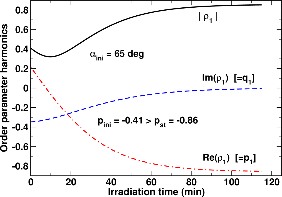
(a) Order parameter harmonics

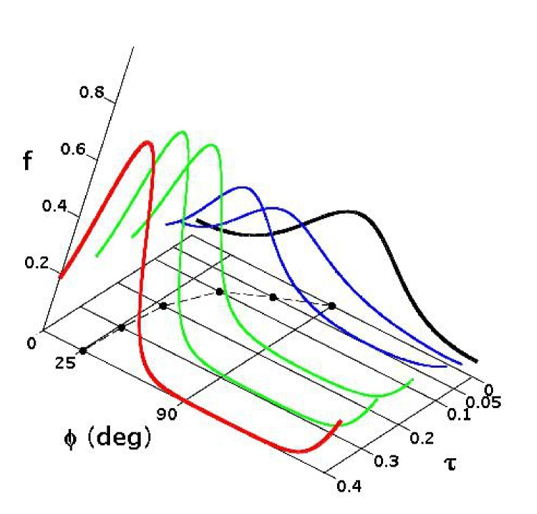
(b) Angular distribution function

Figure 4: (a) Order parameter harmonics, $\rho_{1}$, computed as a function of dimensionless time parameter $\tau$ by numerically solving the initial value problem for the system (22) with the initial angular distribution (43) at $\alpha_{\mathrm{ini}}=65$ deg and $p_{\mathrm{ini}}=-0.41$. The photoexcitation and interaction parameters are: $v_{1}=3$ and $v_{2}=-1$. The stationary state is unique and is characterized by the steady state harmonics $p_{\mathrm{st}}=p_{\mathrm{st}}^{(-)}\approx-0.86$. (b) Angular dependence of the orientational distribution function (46), $f(\phi,\tau)$, at different values of the time parameter, $\tau$. The distribution is $\pi$-periodic and solid circles indicate the angles, $\phi_{\mathrm{max}}=\pi/2-\alpha_{e}$, where peaks are located.

An important conclusion to draw from this result is that, upon reaching the stationary state, the principal axis reorients along the direction perpendicular (parallel) to the polarization vector of the reorienting light, $\hat{\mathbf{e}}_{p}=(-\sin\alpha_{p},\cos\alpha_{p},0)$, with $\alpha_{e}\to\alpha_{e}^{(\mathrm{st})}=\alpha_{p}$ ($\alpha_{e}\to\alpha_{e}^{(\mathrm{st})}=\pi/2+\alpha_{p}$) when the steady state order parameter harmonics is negative (positive), $p_{\mathrm{st}}=p_{\mathrm{st}}^{(-)}<0$ ($p_{\mathrm{st}}=p_{\mathrm{st}}^{(+)}>0$). Thus, in the photosaturated regime, the orientation of azo-dye molecules turned out to be defined solely by the polarization azimuth of the reorienting UV light.

As it has been discussed in Sec. II.2.3, when the activating light is switched off and $I_{UV}=0$ ($v_{1}=0$), the steady states are continuously degenerate with the azimuthal angle of the principal axis playing the role of the degeneracy parameter. The reason for such degeneracy is that the intermolecular interaction is taken in the rotationally invariant Maier-Saupe form (9). The effect of the reorienting linearly polarized light is to lift the degeneracy by breaking the rotational symmetry of the intermolecular interaction.

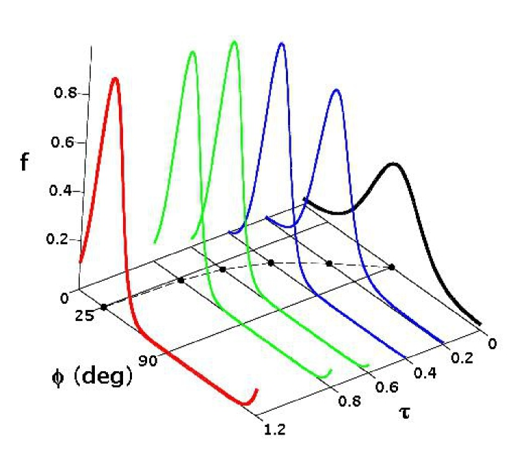
Figure 5: Angular dependence of the orientational distribution function, $f$, within the span of the period computed for various values of the time parameter, $\tau=D_{\mathrm{rot}}t$, at $\alpha_{\mathrm{ini}}=65$ deg and $p_{\mathrm{ini}}=-0.58$. The photoexcitation and interaction parameters are $v_{1}=1.3$ and $v_{2}=-5$, respectively.

III.3 Computational procedure and bistability effects

According to the results of Ref. Kiselev et al. (2005), when the photoaligned azo-dye film is used as an aligning substrate in a NLC cell, orientation of the easy axis at the azo-dye substrate is dictated by the principal axis of the order parameter tensor (24). In particular, under certain conditions, the difference between the angle $\alpha_{e}$ and the easy axis azimuthal angle can be negligible. In this case, the kinetics of the easy axis can be modeled by solving the system (22) and computing the angle $\alpha_{e}$ (see Eq. (30)) as a function of time.

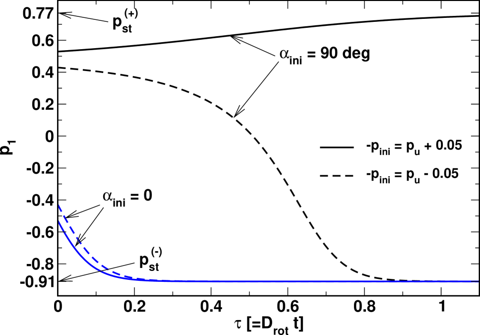
Figure 6: Order parameter harmonics, $p_{1}$, computed as a function of time parameter, $\tau=D_{\mathrm{rot}}t$, by numerically solving the initial value problem for the system (22) with the initial angular distribution (43) at $\alpha_{\mathrm{ini}}=90$ deg and $\alpha_{\mathrm{ini}}=0.0$ deg for $-p_{\mathrm{ini}}=p_{u}\pm 0.05$. The photoexcitation and interaction parameters are: $v_{1}=1.3$ and $v_{2}=-5$. The stationary states are characterized by the steady state harmonics: $p_{\mathrm{st}}^{(-)}\approx-0.91$, $p_{\mathrm{st}}^{(+)}\approx 0.77$ and $p_{u}\approx 0.48$.

In our modeling, we numerically solve the initial value problem for the harmonics $\tilde{\rho}_{k}$ with the initial angular distribution

$$\tilde{f}_{\mathrm{ini}}\propto\exp[-v_{\mathrm{ini}}\cos 2(\phi-\phi_{\mathrm{ini}})].$$ (43)

The distribution (43) is characterized by the initial value of the order parameter harmonics $\rho_{1}^{(\mathrm{ini})}=p_{\mathrm{ini}}=-I_{1}(v_{\mathrm{ini}})/I_{0}(v_{\mathrm{ini}})$ that gives the coupling coefficient $v_{\mathrm{ini}}$. At the initial instant of time, the harmonics are thus given by

$$\tilde{\rho}_{k}(0)=\exp[2ik\alpha_{\mathrm{ini}}](-1)^{k}I_{k}(v_{\mathrm{ini}})/I_{0}(v_{\mathrm{ini}}).$$ (44)

In particular, for the order parameter harmonics, we have

$$\tilde{p}_{1}(0)=p_{\mathrm{ini}}\cos(2\alpha_{\mathrm{ini}}),\quad\tilde{q}_{1}(0)=p_{\mathrm{ini}}\sin(2\alpha_{\mathrm{ini}}).$$ (45)

The initial data defined in Eqs. (43) and (44) represent the angular distribution of azo-dye molecules formed in the film after the preparatory stage of initial irradiation with linearly polarized UV light, $\mathbf{E}_{\mathrm{ini}}$. Note that, when the polarization vector $\mathbf{E}_{\mathrm{ini}}$ is parallel to the $y$ axis, the angle $\alpha_{\mathrm{ini}}$ is equal to the polarization azimuth of the reorienting light $\alpha_{p}$.

The system (22) with the coupling coefficient $v=\tilde{v}=v_{1}+v_{2}\tilde{\rho}_{1}$ describes how the harmonics evolve in time approaching, in the long time limit, the steady state values given in Eq. (35). These values are determined by the steady state order parameter harmonics that can be found by solving the self-consistency equation (36)

At sufficiently large positive photoexcitation parameter, $v_{1}>|v_{c}|$, the equilibrium (photosteady) state is unique and is characterized by the steady state order parameter harmonics $p_{\mathrm{st}}^{(-)}$. This case is illustrated in figure 4a that shows how the order parameter harmonics, $\tilde{\rho}_{1}=p_{1}+iq_{1}$, relaxes to the equilibrium state, $p_{1}(t)\to p_{\mathrm{st}}^{(-)}<0$ and $q_{1}(t)\to 0$ at $t\to\infty$. The equilibrium value of the principle (easy) axis angle (30) then equals the polarization azimuth $\alpha_{p}$ and $\alpha_{e}(t)\to\alpha_{p}$. The latter implies that, in the regime of photosaturation, the azo-dye molecules align perpendicular to the polarization vector of the reorienting, $\hat{\mathbf{n}}_{e}\to(\cos\alpha_{p},\sin\alpha_{p},0)\perp\mathbf{E}_{UV}$. Such behavior is in complete agreement with our experimental data described in Sec. IV and has been previously observed in a number of experimental studies (see, e.g., the monograph Chigrinov et al. (2008) and references therein).

Figure 4a additionally illustrates that the magnitude of the order parameter harmonics, $|\rho_{1}|$, related to the scalar order parameter, $s_{+}$, given in Eq. (42a) can be a nonmonotonic function of time. For the angular distribution function

$$f(\phi,\tau)=(2\pi)^{-1}\sum_{k=-\infty}^{\infty}\tilde{\rho}_{k}(\tau)\exp[-2ik(\phi+\alpha_{p})]$$ (46)

this implies that the distribution may experience broadening at the early stage of relaxation whereas it is getting narrower during the subsequent relaxation to the highly ordered photosteady state. The effect of early stage disordering can be seen in Fig. 4b that shows how the orientational distribution function (46) of azo-dye molecules evolves in time. Note, however, that such transient disordering is typically either less pronounced or completely suppressed. The latter case is demonstrated in Fig. 5.

Temporal evolution of the angular distribution shown in Fig. 5 is computed in the bistability region where the intermolecular interaction parameter, $v_{2}$, is below its critical value, $v_{2}^{(c)}=-2$, and the photoexcitation parameter, $v_{1}>0$, is sufficiently small, $v_{1}<|v_{c}|$ (see Eq. (38)). This is the region where, in addition to the equilibrium state with the negative order parameter harmonics $\tilde{\rho}_{1}=p_{\mathrm{st}}^{(-)}$, the metastable state with the harmonics of opposite sign $\tilde{\rho}_{1}=p_{\mathrm{st}}^{(+)}$ is formed.

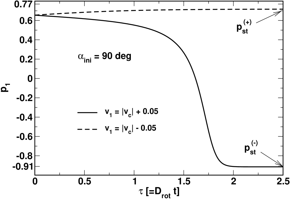
Figure 7: Order parameter harmonics, $p_{1}$, computed as a function of time parameter, $\tau=D_{\mathrm{rot}}t$, by numerically solving the initial value problem for the system (22) with the initial angular distribution (43) at $\alpha_{\mathrm{ini}}=90$ deg and $-p_{\mathrm{ini}}=0.65$ for $v_{1}=|v_{c}|\pm 0.05$. The interaction parameter and the critical value of the photoexcitation parameter are: $v_{2}=-5$ and $|v_{c}|\approx 1.51$, respectively.

Hence the stationary state free energy (34) takes the form of double-well potential with two local minima located at $p_{\mathrm{st}}^{(-)}$ and $p_{\mathrm{st}}^{(+)}$. There is also a local maximum peaked at the point $p_{u}$ in the interval ranged from $p_{\mathrm{st}}^{(-)}$ to $p_{\mathrm{st}}^{(+)}$. Referring to Fig. 2(a), at $v_{1}>0$, this point with $p_{u}>0$ lies on the upper half part of the branch representing unstable stationary states. In the case of real valued harmonics with $q_{k}=0$, it is the boundary point of the basins of attraction of the two steady states. In particular, this means that the order parameter harmonics $p_{1}$ converges to either $p_{\mathrm{st}}^{(-)}$ or $p_{\mathrm{st}}^{(+)}$ depending on whether its initial value $p_{1}(0)$ is below or above the boundary value $p_{u}$.

At $\alpha_{\mathrm{ini}}=0$ and $\alpha_{\mathrm{ini}}=\pi/2$, the initial data (44) are represented by two sets of real valued harmonics. From Eq. (44) it is evident that the only difference between the sets is the sign of the odd numbered harmonics . In particular, we have $p_{1}(0)=p_{\mathrm{ini}}$ and $p_{1}(0)=-p_{\mathrm{ini}}$ at $\alpha_{\mathrm{ini}}=\alpha_{p}=0$ and $\alpha_{\mathrm{ini}}=\pi/2$, respectively.

At $\alpha_{\mathrm{ini}}=0$ and $p_{\mathrm{ini}}<0$, the harmonics characterizing the equilibrium state, $p_{\mathrm{st}}^{(-)}$, is the attracting point for the order parameter harmonics and the azimuthal angle of the principal (easy) axis, remains intact, $\alpha_{e}^{(\mathrm{st})}=0$. The latter comes as no surprise because the polarization vectors of the initial irradiation and of the reorienting light are parallel, $\mathbf{E}_{UV}\parallel\mathbf{E}_{\mathrm{ini}}$

Interestingly, orientation of the easy axis may stay unchanged even if the vectors, $\mathbf{E}_{UV}$ and $\mathbf{E}_{\mathrm{ini}}$, are perpendicular and $\alpha_{\mathrm{ini}}=\alpha_{p}=\pi/2$. This occurs when the initial ordering is high, so that $-p_{\mathrm{ini}}$ is greater than $p_{u}$, $-p_{\mathrm{ini}}>p_{u}$. As demonstrated in Fig. 6, in this case, the attracting point is the metastable harmonics $p_{\mathrm{st}}^{(+)}$ rather than the equilibrium one $p_{\mathrm{st}}^{(-)}$ and $\alpha_{e}^{(\mathrm{st})}=0$.

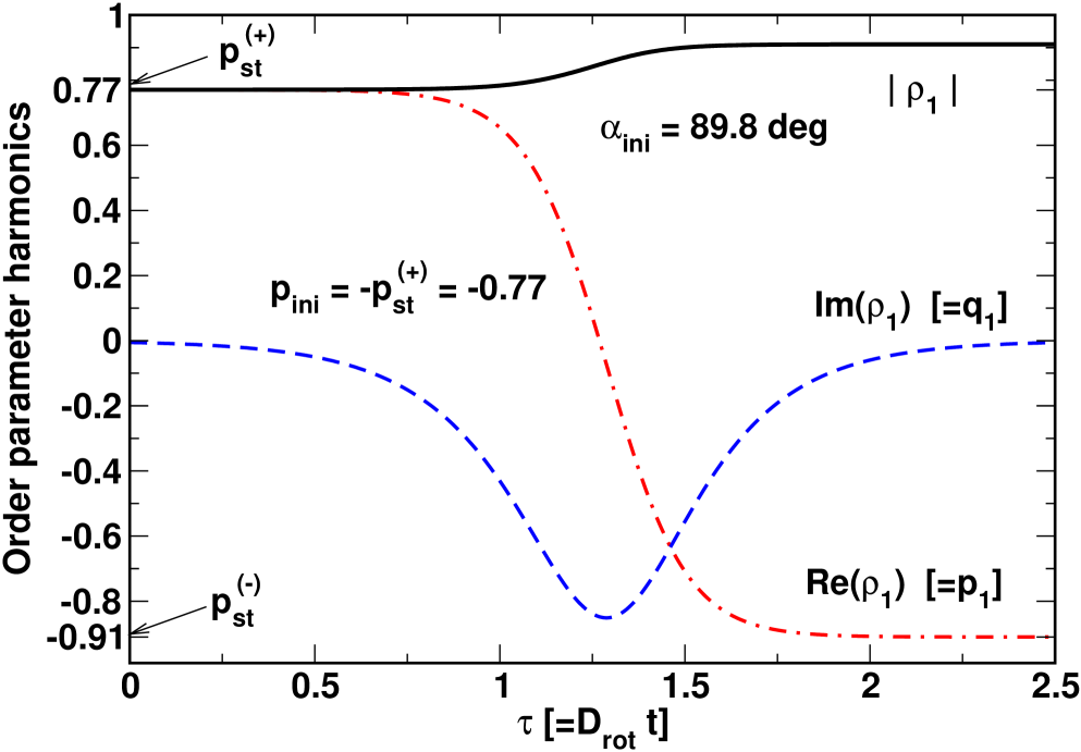
Figure 8: Order parameter harmonics, $\rho_{1}$, computed as a function of time parameter, $\tau=D_{\mathrm{rot}}t$, at $\alpha_{\mathrm{ini}}=89.8$ deg and $p_{\mathrm{ini}}=-p_{\mathrm{st}}^{(+)}$. Other parameters are listed in the caption of Fig. 6.

It can also be seen from the curves of Fig. 6 that, in the opposite case of low ordered initial states with $-p_{\mathrm{ini}}<p_{u}$, the order parameter harmonics $p_{1}$ relaxes back to the equilibrium value $p_{\mathrm{st}}^{(-)}$. So, at $-p_{\mathrm{ini}}<p_{u}$, the azimuthal angle, $\alpha_{e}^{(\mathrm{st})}=\alpha_{p}=\pi/2$, defines the steady state easy axis which is normal to the direction of its initial orientation.

In Fig. 7, we show that, when the initial ordering is sufficiently high, the process of reorientation crucially depends on whether the photoexcitation parameter, $v_{1}$, which is proportional to the intensity of the reorienting light, $I_{UV}$, exceeds its critical value, $|v_{c}|$. This critical value determines the intensity threshold, $I_{c}=4|v_{c}/(3u_{I})|$, and the easy axis reorientation is suppressed at $\alpha_{p}=\pi/2$ in the low intensity region below the threshold where $I_{UV}<I_{c}$.

Similar threshold behavior has been previously observed in a number of experimental studies on light-induced easy axis reorientation in nematic liquid crystal cells with photosensitive polymer substrates Dyadyusha et al. (1992); Voloshchenko et al. (1995); Andrienko et al. (1998); Chigrinov et al. (2008). For azo-dye films, the experimental data of Refs. Dubtsov et al. (2010, 2012) also suggest the presence of a threshold when the polarization vector $\mathbf{E}_{UV}$ is directed along the initial easy axis (see the subsequent section for more details). Our result that under certain conditions highly ordered initial distributions may relax to the metastable stationary state offers a possible explanation for this.

Referring to Fig. 8, it is seen that small deviations of the angle $\alpha_{\mathrm{ini}}$ from $\pi/2$ have a destructive effect on metastability of the attracting point even if $-p_{\mathrm{ini}}=p_{\mathrm{st}}^{(+)}$. It turned out that the basin of attraction of the metastable state is unstable with respect to fluctuations of the polarization azimuth $\alpha_{p}$. In the vicinity of the critical angle $\alpha_{\mathrm{ini}}=\pi/2$, the presence of the metastable state manifests itself as appreciably retarded relaxation to the equilibrium state (see Fig. 8). Similarly, the shape of the azimuthal angle (30) vs time curve shown in Fig. 9 points to a time delay in the process of principal (easy) axis reorientation.

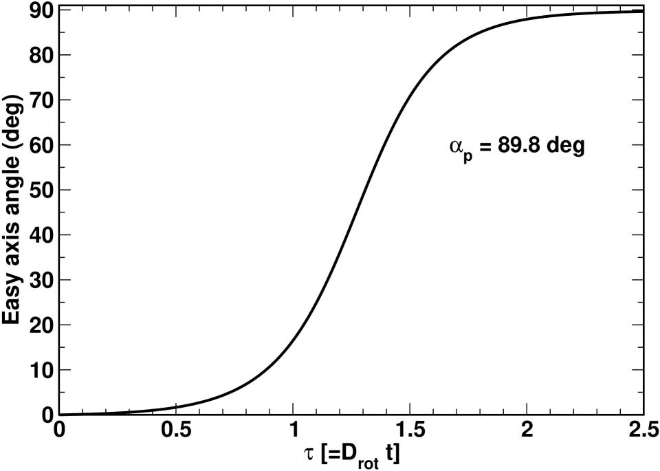
Figure 9: Principal axis azimuthal angle, $\alpha_{e}$, computed as a function of time parameter, $\tau=D_{\mathrm{rot}}t$, at $\alpha_{\mathrm{ini}}=\alpha_{p}=89.8$ deg and $p_{\mathrm{ini}}=-p_{\mathrm{st}}^{(+)}$. Other parameters are listed in the caption of Fig. 6.

IV Theory versus experiment

In the previous section we have examined the experimentally important predictions of the model. These predictions can, in principle, be tested and, in this section, we discuss some of our recent experimental results on the reorientational dynamics of the electrically assisted light-induced azimuthal gliding of the easy axis at varying polarization azimuth of LPUV reorienting light Dubtsov et al. (2012).

Such gliding is found to take place on photoaligned azo-dye layers when irradiation of nematic LC (NLC) cells with LPUV light is combined with the application of ac in-plane electric field Pasechnik et al. (2008); Dubtsov et al. (2010). Since the effects of electric field is well beyond the scope of the theoretical approach under consideration, the regime of purely light-induced reorientation will be our primary concern and we deal with the data measured in the electric field-free regions

In our experiments, LC cells ($d=17.4\pm 0.2\,\mu$m) of sandwich like type were assembled between two amorphous glass plates. The upper glass plate was covered with a rubbed polyimide film giving the strong planar anchoring conditions. A film of the azobenzene sulfric dye SD1 (Dainippon Ink and Chemicals) Chigrinov et al. (2008) was deposited onto the bottom substrate on which transparent indium tin oxide (ITO) electrodes were placed. The electrodes and the interelectrode stripes (the gap was about $g=50\leavevmode\nobreak\ \mu$m and the in-plane ac voltage was $U=100$ V with $f=3$ kHz) were arranged to be parallel to the direction of rubbing (the $x$ axis).

The azo-dye SD1 layer was initially illuminated by LPUV light at the wavelength $\lambda=365$ nm. The preliminary irradiation produced the zones of different energy dose exposure $D_{p}=0.27,\,0.55$ J/cm² characterized by relatively weak azimuthal anchoring strength. The light propagating along the normal to the substrates (the $z$ axis) was selected by an interference filter. Initial orientation of the polarization vector of the actinic light, $\mathbf{E}_{\mathrm{ini}}$, was chosen so as to align azo-dye molecules at a small angle of 4 degrees to the $x$ axis, $\varphi_{0}\approx 4$ deg.

The LC cell was filled with the nematic LC mixture E7 (Merck) in isotropic phase and then slowly cooled down to room temperature. Thus we prepared the LC cell with a weakly twisted planar orientational structure where the director at the bottom surface $\mathbf{n}_{0}$ is clockwise rotated through the initial twist angle $\varphi_{0}\approx 4$ deg which is the angle between $\mathbf{n}_{0}$ and the director at the upper substrate (the $x$ axis).

In addition to the electric field, $E=2$ V/$\mu$m, the cell was irradiated with the reorienting LPUV light beam ($I_{UV}=0.26$ mW/cm² and $\lambda=365$ nm) normally impinging onto the bottom substrate. For this secondary LPUV irradiation, orientation of the polarization plane is determined by the polarization azimuth, $\alpha_{p}$.

Our experimental method has already been described in Refs. Pasechnik et al. (2008); Dubtsov et al. (2010). In this method, NLC orientational structures were observed via a polarizing microscope connected with a digital camera and a fiber optics spectrometer. The rotating polarizer technique was used to measure the azimuthal angle $\varphi_{e}$ characterizing orientation of the easy axis. In order to register microscopic images and to measure the value of $\varphi_{e}$, the electric field and the reorienting light were switched off for about 1 min. This time interval is short enough to ensure that orientation of the easy axis remains essentially intact in the course of measurements. The measurements were carried out at a temperature of 26^∘C.

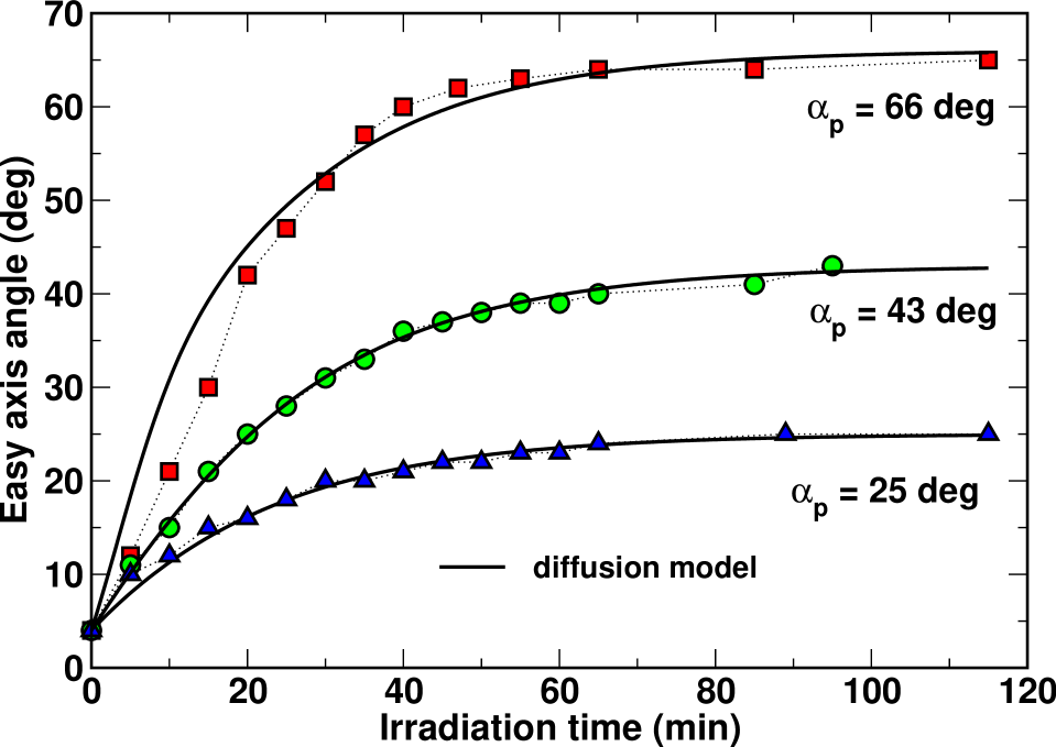
Figure 10: Easy axis angle versus the irradiation time at different values of the polarization azimuthal angle of the reorienting UV light $\alpha_{p}$. The experimental data were measured by using the linearly polarized activating light with $\lambda=365$ nm and $I=2.6$ W/m². Solid lines represent the theoretical curves computed by numerically solving the initial value problem for the system (22) with the initial angular distribution (43). The parameters used in calculations are as follows: the photoexcitation (interaction) parameter is $v_{1}=1.3$ ($v_{2}=-5$); $p_{\mathrm{ini}}=p_{\mathrm{st}}^{(-)}$ ($\alpha_{p}=25$ deg and $\alpha_{p}=43$ deg) and $p_{\mathrm{ini}}=-0.25$ at $\alpha_{p}=65$ deg. Other parameters are listed in the caption of Fig. 6.

The case where the reorienting light is linearly polarized along the initial surface director $\mathbf{n}_{0}$ and $\alpha_{p}=\pi/2$, was studied in Refs. Pasechnik et al. (2008); Dubtsov et al. (2010). It turned out that, by contrast to the electrically assisted light-induced gliding, the purely photoinduced reorientation is almost entirely inhibited at $\alpha_{p}=\pi/2$. As it can be seen from Fig. 10, the latter is no longer the case for the reorienting light with $\alpha_{p}\neq\pi/2$.

Thus the result is that, as opposed to the cases with non-vanishing electric field and $\alpha_{p}\neq\pi/2$, the purely photoinduced reorientation of the easy axis has been completely suppressed when the polarization plane is parallel to the initial easy axis. From the above discussion, our model predicts similar behavior that occurs in the bistability region where the reorientation is characterized by the threshold for the intensity of reorienting light.

Figure 10 shows the easy axis angle measured as a function of the irradiation time at various values of the polarization azimuth. The measurements were performed in the region outside the interelectrode gaps where the ac electric field is negligibly small. In the zero-field curves, the easy axis angle increases with the irradiation time starting from the angle of initial twist, $\varphi_{0}$, and approaches the photosteady state characterized by the photosaturated value of the angle close to $\alpha_{p}$.

The experimental data can be fitted by the theoretical curves computed from the formula (30), where the order parameter harmonics, $\tilde{\rho}_{1}$, is found by numerically solving the initial value problem for the system (22) with the initial angular distribution (43). In Fig. 10 we make a comparison between the experimental data and the theoretical curves computed in the bistability region by setting the photoexcitation and interaction parameters, $v_{1}$ and $v_{2}$, equal to $1.3$ and $-5$, respectively. In this region, the equilibrium state is characterized by the steady state harmonics $p_{\mathrm{st}}=p_{\mathrm{st}}^{(-)}\approx-0.91$, whereas the stationary harmonics $p_{\mathrm{st}}^{(+)}\approx 0.77$ corresponds to the metastable state. For $\alpha_{p}=25$ deg and $\alpha_{p}=43$ deg, the curves were computed at $p_{\mathrm{ini}}=p_{\mathrm{st}}^{(-)}$. It follows that $|\rho_{1}(0)|=|\rho_{\mathrm{st}}|$ and the angle $\alpha_{\mathrm{ini}}$ is assumed to be the only parameter describing difference between the initial and the equilibrium angular distributions. The rotational diffusion coefficient $D_{\mathrm{rot}}$ can be estimated at about $1.6\times 10^{-4}$ s^-1 Using this value to fit the data measured at $\alpha_{p}=65$ deg, we find that the theoretical and experimental results are in agreement when the initial ordering parameter $p_{\mathrm{ini}}\approx-0.25$ differs from the equilibrium value.

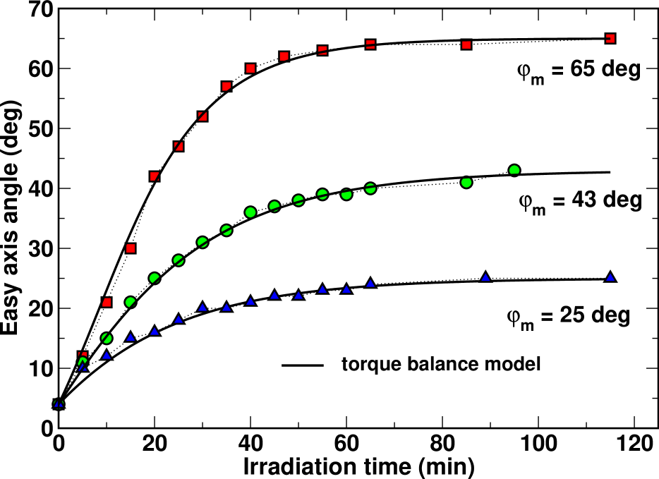
Figure 11: Easy axis angle versus the irradiation time in the electric field-free region at different values of the polarization azimuthal angle of the reorienting UV light. The experimental data were measured by using the linearly polarized activating light with $\lambda=365$ nm and $I=2.6$ W/m². Solid lines represent the theoretical curves computed from the formula (48) at $t_{e}=\gamma_{e}/W_{e}=23$ min (for $\varphi_{m}=25$ deg and $\varphi_{m}=43$ deg), and $t_{e}\approx 14.4$ min. for $\varphi_{m}=65$ deg.

We conclude this section with the remark concerning the phenomenological model formulated in Refs. Pasechnik et al. (2006, 2008) to describe the effect of the electrically assisted photoinduced gliding of the easy axis. According to this model, in the absence of ac electric field, temporal evolution of the easy axis azimuthal angle $\varphi_{e}$ can be described by the balance torque equation Dubtsov et al. (2012)

$$\gamma_{e}\frac{\partial\varphi_{e}}{\partial t}=-\frac{W_{e}}{2}\sin 2(\varphi_{e}-\varphi_{m}),$$ (47)

where $\gamma_{e}$ is the specific viscosity of gliding; $W_{e}$ is the effective anchoring parameter which defines the strength of coupling between the easy axis $\mathbf{n}_{e}$ and the initial state of surface orientation; $\varphi_{m}$ is the polarization dependent phase shift. The solution of the dynamic equation (47)

$$\tan(\varphi_{e}(t)-\varphi_{m})=\tan(\varphi_{e}(0)-\varphi_{m})\exp[-t/t_{e}],$$ (48)

where $t_{e}=\gamma_{e}/W_{e}$ the characteristic time of easy axis reorientation, can now be used to fit the experimental data. The results are presented in Fig. 11.

From the curves depicted in Fig. 11 it can be inferred that the phase shift $\varphi_{m}$ is close to the polarization azimuth of the reorienting light. The value of the characteristic time, $t_{e}\approx 14.4$ min, estimated for $\varphi_{m}=65$ deg differs from the one $t_{e}\approx 23$ min obtained for other two angles, $\varphi_{m}=25$ deg and $\varphi_{m}=43$ deg. From the other hand, in Fig. 10, the case with $\alpha_{p}\approx 65$ deg is distinctive in initial ordering of the film. This result points to the fact that the coupling strength of the easy axis $W_{e}$ depends on the photoinduced order parameter of the initially irradiated azo-dye layer. Such dependence was one of the key assumptions taken in Ref. Dubtsov et al. (2010) when applying the phenomenological model Pasechnik et al. (2006, 2008) to interpret the experimental data for photoaligned azo-dye layers prepared at different initial irradiation doses.

V Discussion and conclusions

In this paper we have studied the kinetics of orientational reordering that takes place in the azo-dye films under the action of LPUV reorienting light. In our theoretical approach, the process of reordering is described in terms of a rotational Brownian motion and we have employed the 2D diffusion model formulated in Ref. Kiselev et al. (2009) to explore the peculiarities of the photoinduced reordering in the regime of purely in-plane reorientation.

Orientational ordering of azo-dye molecules is characterized by the in-plane (2D) order parameter tensor (24). This tensor is expressed in terms of the order parameter harmonics, $\rho_{1}$, that enters the formula (25) giving both the value of the scalar order parameter, $s_{+}$, and the azimuthal angle, $\alpha_{e}$, of the principal (easy) axis, $\hat{\mathbf{n}}_{e}$.

It is found that dynamics of the order parameter harmonics essentially depends on the initial ordering and the polarization azimuth of the LP reorienting light. In the long time limit, the order parameter harmonics approaches its steady state value reaching the regime of photosaturation. We have proved that, in the steady state, the easy axis azimuthal angle is dictated solely by the polarization azimuth, $\alpha_{p}$, (see Eq. (42)), whereas the photostationary value of the scalar order parameter is determined by the photoexcitation and intermolecular interaction parameters, $v_{1}\propto I_{UV}$ and $v_{2}$, defined in Eq. (19c).

In the $v_{1}$-$v_{2}$ plane, inequalities (38) define the bistability region (see Fig. 2(b)) with two locally stable stationary states: equilibrium and metastable ones. An experimentally important bistability effect is that the easy axis reorientation is inhibited when the intensity of the reorienting light linearly polarization along the initial easy axis is below its critical (threshold) value. Such threshold behavior was observed in our experiments where the easy axis angle was measured as a function of the irradiation time at varying polarization azimuth of LPUV reorienting light.

An alternative phenomenological model that also predicts the presence of the reorientation threshold was suggested in Ref. Alexe-Ionescu et al. (2007). In that model, the threshold effect comes about from the interplay between two competing easy axes. By contrast, in our model, the bistability appears as an intrinsic property of the reordering process in azo-dye films that manifests itself as the threshold of reorientation.

There is another interesting bistability effect that occurs when the light is switched off ($I_{UV}=0$) and $v_{2}<v_{2}^{(c)}=-2$. In this case, owing to the rotational symmetry of the two-particle interaction (9), the easy axis angle, $\alpha_{e}$, becomes undetermined and plays the role of the degeneracy parameter. The LPUV light field lifts the degeneracy and the dynamics of the angle turned out to be predominately governed by the photoexcitation parameter, $v_{1}$.

For the scalar order parameter which is related to the magnitude of the order parameter harmonics, $|\rho_{1}|$, the rate of relaxation is typically at least twice faster than that for the easy axis angle. As is illustrated in Fig. 4a, depending on the initial conditions, temporal evolution of this order parameter can be non-monotonic. These effects can also be seen from Figs. 4b and 5 that show how the orientational angular distribution of azo-dye molecules evolves in time.

By numerically solving the dynamical system for the angular distribution harmonics (22) we have fitted the experimental data on the light-induced azimuthal gliding of the easy axis at the photoaligned azo-dye SD1 layer. In our analysis, the photoinduced reordering of azo-dye molecules was assumed to be the key factor dominating the easy axis reorientation.

Despite the fact that good agreement between the computed curves and the data (see Fig. 10) counts in favor of our simplified approach, a deeper insight into complicated molecular mechanisms behind the gliding under consideration requires additional experimental studies and a more systematic theoretical treatment of the processes involved. Such treatment has to deal with the interplay of photoinduced ordering in azo-dye films, the anchoring energy effects Kiselev et al. (2005) and the adsorption-desorption processes Vetter et al. (1993); Ouskova et al. (2001); Barbero and Evangelista (2006); Fedorenko et al. (2008) underlying the gliding phenomenon.

This work was partially supported by grants: Development of the Higher School’s Scientific Potential 2.1.1/5873; Grant NK-410P; HKUST CERG RPC07/08.EG01 and CERG 612208, 612409.

References

- Zhao and Ikeda (2009) Yue Zhao and Tomiki Ikeda, eds., Smart light-responsive materials: Azobenzene-containing polymers and liquid crystals (Wiley, New Jersey, USA, 2009) p. 514.
- Weigert (1919) F. Weigert, “A new effect of the rays in light-sensitive layers,” Verh. Dtsch. Phys. Ges. 21, 479–491 (1919).
- Eich et al. (1987) M. Eich, J. H. Wendorff, B. Reck, and H. Ringsdorf, “Reversible digital and holographic optical storage in polymeric liquid crystals,” Makromol. Chem., Rap. Commun. 8, 59–63 (1987).
- Natansohn et al. (1992) A. Natansohn, S. Xie, and P. Rochon, “Azo polymers for reversible optical storage. 2. Poly[-[[2-(acryloyloxy)ethyl]ethylamino]-2-chloro-4-nitroazobenzene],” Macromolecules 25, 5531–5532 (1992).
- Prasad et al. (1995) P. N. Prasad, J. E. Mark, and T. J. Fai, eds., Polymers and other advanced materials (Plemun Press, NY, 1995).
- Blinov et al. (1999) L. M. Blinov, M. V. Kozlovsky, and G. Cipparrone, “Photochromism and holographic grating recording on a chiral side-chain liquid crystalline copolymer containing azobenzene chromophores,” Chem. Phys. 245, 473–485 (1999).
- Yang and Wu (2006) D.-K. Yang and S.-T. Wu, Fundamentals of Liquid Crystal Devices, Series in Display Technology (Wiley, Chichester, 2006) p. 378.
- Chigrinov et al. (2008) V. G. Chigrinov, V. M. Kozenkov, and H.-S. Kwok, Photoalignment of Liquid Crystalline Materials: Physics and Applications, Series in Display Technology (Wiley, Chichester, 2008) p. 219.
- O’Neill and Kelly (2000) M. O’Neill and S. M. Kelly, “Photoinduced surface photoalignment for liquid crystal displays,” J. Phys. D: Appl. Phys. 33, R67–R84 (2000).
- Chigrinov et al. (2003a) V. G. Chigrinov, V. M. Kozenkov, and H. S. Kwok, “New developments in photo-aligning and photo-patterning technologies: physics and applications,” in Optical applications in photoaligning, edited by L. Vicari (Inst. of Physics, Bristol, UK, 2003) pp. 201–244.
- Gibbons et al. (1991) W. M. Gibbons, P. J. Shannon, S.-T. Sun, and B. J. Swetlin, “Surface-mediated alignment of nematic liquid crystals with polarized laser light,” Nature 351, 49–50 (1991).
- Furumi et al. (1999) S. Furumi, M. Nakagawa, S. Morino, and K. Ichimura, “Photogeneration of high pretilt angles of nematic liquid crystals by azobenzene-containing polymer films,” Appl. Phys. Lett. 74, 2438–2440 (1999).
- Schadt et al. (1992) M. Schadt, K. Schmitt, V. Kozinkov, and V. Chigrinov, “Surface-induced parallel alignment of liquid crystals by linearly polymerized photopolymers,” Jpn. J. Appl. Phys. 31, 2155–2164 (1992).
- Dyadyusha et al. (1992) A. G. Dyadyusha, T. Ya. Marusii, Yu. A. Reznikov, A. I. Khizhnyak, and V. Yu. Reshetnyak, “Orientational effect due to a change in the anisotropy of the interaction between a liquid crystal and a bounding surface,” JETP Lett. 56, 17 (1992).
- Galabova et al. (1996) H. G. Galabova, D. W. Allender, and J. Chen, “Orientation and surface anchoring of nematic liquid crystals on linearly polymerized photopolymers,” Phys. Rev. E 55, 1627–1631 (1996).
- Perny et al. (2000) S. Perny, P. Le Barny, J. Delaire, T. Buffeteau, C. Sourisseau, I. Dozov, S. Forget, and P. Martinot-Lagarde, “Photoinduced orientation in poly(vinylcinnamate) and poly(7-methacryloyloxycoumarin) thin films and the consequences on liquid crystal alignment,” Liq. Cryst. 27, 329–340 (2000).
- Petry et al. (1993) A. Petry, S. Kummer, H. Anneser, F. Feiner, and Ch. Bräuchle, “Photoinduced reorientation of cholesteric liquid crystalline polysiloxinanes and applications in optical information storage and second harmonic,” Ber. Bunsenges. Phys. Chem. 97, 1281–1286 (1993).
- Holme et al. (1996) N. C. R. Holme, P. S. Ramanujam, and S. Hvilsted, “Photoinduced anisotropy measurements in liquid-crystalline azobenzene side-chain polyesters,” Applied Optics 35, 4622–4627 (1996).
- Blinov et al. (1998) L. Blinov, M. Kozlovsky, M. Ozaki, K. Skarp, and K. Yoshino, “Photoinduced dichroism and optical anisotropy in a liquid-crystalline azobenzene side chain polymer caused by anisotropic angular distribution of trans and cis isomers,” J. Appl. Phys. 84, 3860–3866 (1998).
- Wu et al. (2000) Y. Wu, J.-I. Mamiya, O. Tsutsumi, A. Kanazawa, T. Shiono, and T. Ikeda, “Photoinduced alignment of polymer liquid crystals containing azobenzene moieties in the side group VII. On He-Ne laser beam irradiation,” Liq. Cryst. 27, 749–753 (2000).
- Wiesner et al. (1992) U. Wiesner, N. Reynolds, Ch. Boeffel, and H. W. Spiess, “An infrared spectroscopic study of photo-induced reorientation in dye containing liquid-crystalline polymers,” Liq. Cryst. 11, 251–267 (1992).
- Yaroshchuk et al. (2001) O. Yaroshchuk, A. D. Kiselev, Yu. Zakrevskyy, J. Stumpe, and J. Lindau, “Spatial reorientation of azobenzene side groups of a liquid crystalline polymer induced by linearly polarized light,” Eur. Phys. J. E 6, 57–67 (2001).
- Pedersen and Johansen (1997) T. G. Pedersen and P. M. Johansen, “Mean-field theory of photoinduced molecular reorientation in azobenzene liquid crystalline side-chain polymers,” Phys. Rev. Lett. 79, 2470–2473 (1997).
- Pedersen et al. (1998) T. G. Pedersen, P. M. Johansen, N. C. R. Holme, P. S. Ramanujam, and S. Hvilsted, “Theoretical model of photoinduced anisotropy in liquid crystalline azobenzene side-chain polyesters,” J. Opt. Soc. Am. B 15, 1120–1129 (1998).
- Puchkovs’ka et al. (1998) G. A. Puchkovs’ka, V. Yu. Reshetnyak, A. G. Tereshchenko, O. V. Yaroshchuk, and J. Lindau, “Kinetic characteristics of light induced anisotropy and mechanisms of the molecular alignment in azo dye containing polymer films,” Mol. Cryst. Liq. Cryst. 321, 31–43 (1998).
- Sajti et al. (2001) Sz. Sajti, Á. Kerekes, M. Barabás, E. Lörincz, S. Hvilsted, and P. S. Ramanujam, “Simulation of erasure of photoinduced anisotropy by circularly polarized light,” Opt. Commun. 194, 435–442 (2001).
- Kiselev (2002) A. D. Kiselev, “Kinetics of photoinduced anisotropy in azopolymers: models and mechanisms,” J. Phys.: Condens. Matter 14, 13417–13428 (2002).
- Sekkat et al. (2002) Z. Sekkat, D. Yasumatsu, and S. Kawata, “Pure photoorientation of azo dye in polyurethanes and quantification of orientation of spectrally overlapping isomers,” Journal of Physical Chemistry B 106, 12407–12417 (2002).
- Natansohn et al. (1998) A. Natansohn, P. Rochon, X. Meng, C. Barett, T. Buffeteau, S. Bonenfant, and M. Pezolet, Macromolecules 31, 1155 (1998).
- Buffeteau and Pézolet (1998) T. Buffeteau and M. Pézolet, “Photoinduced orientation in azopolymers studied by infrared spectroscopy: cooperative and biaxial orientation in semicrystalline polymers,” Macromolecules 31, 2631–2635 (1998).
- Kiselev et al. (2001) A. Kiselev, O. Yaroshchuk, Yu. Zakrevskyy, and A. Tereshchenko, “On biaxiality of photoinduced structures in azopolymer films,” Condens. Matter Phys. 4, 67–75 (2001).
- Yaroshchuk et al. (2003) O. V. Yaroshchuk, A. D. Kiselev, Yu. Zakrevskyy, T. Bidna, J. Kelly, L.-C. Chien, and J. Lindau, “Photoinduced three-dimensional order in side chain liquid crystalline azopolymers,” Phys. Rev. E 68, 011803–(1–15) (2003).
- Kaanumalle et al. (2005) L. S. Kaanumalle, A. Natarayan, and V. Ramamurthy, “Medium effects on photochemical processes: Organized and confined media,” in Synthetic Organic Chemistry, Molecular and supramolecular photochemistry, Vol. 12, edited by G. G. Axel and J. Mattay (Marcel Dekker, NY, 2005) Chap. 18, pp. 553–618.
- Kiselev et al. (2008) A. D. Kiselev, V. G. Chigrinov, H.-S. Kwok, An. Murauski, and Al. Muravsky, “Biaxiality effects in kinetics of photoinduced orientational structures in azo-dye films,” in Proceedings of the VIII-th International Display Workshop’08 (SID, Nigata, Japan, 2008) pp. 573–574.
- Kiselev et al. (2009) A. D. Kiselev, V. G. Chigrinov, and H.-S. Kwok, “Kinetics of photoinduced ordering in azo-dye films: Two-state and diffusion models,” Phys. Rev. E 80, 011706 (2009).
- Chigrinov et al. (2002) V. Chigrinov, E. Prudnikova, V. Kozenkov, H. Kwok, H. Akiyama, T. Kawara, H. Takada, and H. Takatsu, “Syntesis and properties of azo dye aligning layers for liquid crystal cells,” Liq. Cryst. 29, 1321–1327 (2002).
- Chigrinov et al. (2003b) V. Chigrinov, A. Muravski, and H. S. Kwok, “Anchoring properties of photoaligned azo-dye materials,” Phys. Rev. E 68, 061702 (2003b).
- Kiselev et al. (2005) A. D. Kiselev, V. G. Chigrinov, and D. D. Huang, “Photo-induced ordering and anchoring properties of azo-dye films,” Phys. Rev. E 72, 061703 (2005).
- Muravsky et al. (2008) A. Muravsky, A. Murauski, V. Chigrinov, and H.-S. Kwok, “Light printing of grayscale pixel images on optical rewritable electronic paper,” Jpn. J. Appl. Phys. 47, 6347–6353 (2008).
- Vorflusev et al. (1997) V. P. Vorflusev, H-S Kitzerow, and V. Chigrinov, “Azimuthal surface gliding of a nematic liquid crystal,” Appl. Phys. Lett. 70, 3359 (1997).
- Pasechnik et al. (2006) S. V. Pasechnik, V. G. Chigrinov, D. V. Shmeliova, V. A. Tsvetkov, V. N. Kremenetsky, L. Zhijian, and A. V. Dubtsov, “Slow relaxation processes in nematic liquid crystals at weak surface anchoring,” Liq. Cryst. 33, 175–185 (2006).
- Dubtsov et al. (2012) A. V. Dubtsov, D. V. Shmeliova, S. V. Pasechnik, Alexei D. Kiselev, and V. G. Chigrinov, “Effects of polarization azimuth in dynamics of electrically assisted light-induced gliding of nematic liquid-crystal easy axis,” Appl. Phys. Lett. 100, 141608 (2012).
- de Gennes and Prost (1993) P. G. de Gennes and J. Prost, The Physics of Liquid Crystals (Clarendon Press, Oxford, 1993) p. 596.
- Lauritzen and Zwanzig (1973) J. I. Lauritzen and R. Zwanzig, “Dielectric relaxation of a single axis rotator with two equivalent sites,” Advances in Molecular Relaxation Processes 5, 339–361 (1973).
- Coffey et al. (1993) W. T. Coffey, Yu. P. Kalmykov, E. S. Massawe, and J. T. Waldron, “Exact solution for the correlation times of dielectric relaxation of a single axis rotor with two equivalent sites,” J. Chem. Phys. 99, 4011–4023 (1993).
- Dejárdin et al. (1993) J.-L. Dejárdin, G. Debiais, and A. Ouadjou, “On the dielectric behavior of dielectric relaxation in alternating fields. II. Analytic expressions of nonlinear susceptibilities,” J. Chem. Phys. 98, 8149–8153 (1993).
- Dejárdin and Kalmykov (2000) J.-L. Dejárdin and Yu. P. Kalmykov, “Nonlinear dielectric relaxation of polar molecules in a strong ac electric field: Steady state response,” Phys. Rev. E 61, 1211–1217 (2000).
- Kalmykov and Quinn (1991) Y. P. Kalmykov and K. P. Quinn, “The rotational Brownian motion in a linear molecule and its application to the theory of Kerr effect relaxation,” J. Chem. Phys. 95, 9142–9147 (1991).
- Felderhof (2002) B. U. Felderhof, “Nonlinear response of a dipolar system with rotational diffusion to a rotating field,” Phys. Rev. E 66, 051503 (2002).
- Kalmykov (2001) Y. P. Kalmykov, “Rotational Brownian motion and nonlinear dielectric relaxation asymmetric top molecules in strong electric fields,” Phys. Rev. E 65, 021101 (2001).
- Kalmykov and Titov (2007) Y. P. Kalmykov and S. V. Titov, “Anisotropic rotational diffusion and transient nonlinear responses of rigid macromolecules in a strong external electric field,” J. Chem. Phys. 126, 174903 (2007).
- Nordio and Busolin (1971) P. L. Nordio and P. Busolin, “Electron spin resonance line shapes in partially oriented systems,” J. Chem. Phys. 55, 5485–5490 (1971).
- Tarroni and Zannoni (1991) R. Tarroni and C. Zannoni, “On the rotational diffusion of asymmetric molecules in liquid crystals,” J. Chem. Phys. 95, 4550–4564 (1991).
- Luckhurst and Sanson (1972) G. R. Luckhurst and A. Sanson, “Angular dependent line widths for a spin probe dissolved in a liquid crystal,” Mol. Phys. 24, 1297–1311 (1972).
- Berggren et al. (1993) D. Berggren, R. Tarroni, and C. Zannoni, “Rotational diffusion of uniaxial probes in biaxial liquid crystal phases,” J. Chem. Phys. 99, 6180–6200 (1993).
- Ferrarini et al. (1994) A. Ferrarini, P. L. Nordio, and G. J. Moro, “Diffusion models for molecular motion in uniaxial mesophases,” in The molecular physics of liquid cristals, edited by G. R. Luckhurst and C. A. Veracini (Kluwer Academic, Dordrecht, 1994) pp. 41–69.
- Brognara et al. (2000) A. Brognara, P. Pasini, and C. Zannoni, “Roto-translational diffusion of biaxial probes in uniaxial liquid crystal phases,” J. Chem. Phys. 112, 4836–4848 (2000).
- Nordio and Serge (1979) P. L. Nordio and U. Serge, “Rotational dynamics,” in The molecular physics of liquid cristals, edited by G. R. Luckhurst and G. W. Gray (Academic Press, London, 1979) Chap. 18.
- Moro and Nordio (1984) G. Moro and P. L. Nordio, “Orientation dependent friction in liquid crystals,” Mol. Cryst. Liq. Cryst. 104, 361–376 (1984).
- Dozov et al. (1987) I. Dozov, N. Kirov, and B. Petroff, “Molecular biaxiality and reorientational correlation functions in nematic phases: theory,” Phys. Rev. A 36, 2870–2878 (1987).
- Fontana et al. (1986) M. P. Fontana, B. Rosi, N. Kirov, and I. Dozov, “Molecular orientational motion in liquid crystals: a study by Raman and infrared band-shape analysis,” Phys. Rev. A 33, 4132–4142 (1986).
- Frank (2005) T. D. Frank, Nonlinear Fokker–Planck Equations, edited by H. Haken, Springer Series in Synergetics (Springer, Berlin, Heidelberg, 2005) p. 404.
- Abramowitz and Stegun (1972) M. Abramowitz and I. A. Stegun, eds., Handbook of Mathematical Functions (Dover, New York, 1972).
- Kuznetsov (1998) Yu. A. Kuznetsov, Elements of Applied Bifurcation Theory, 2nd ed., Applied Mathematical Sciences, Vol. 112 (Springer, NY, 1998) p. 592.
- Hale and Kocak (1991) J. K. Hale and H. Kocak, Dynamics and Bifurcations, Texts in Applied Mathematics, Vol. 3 (Springer, NY, 1991) p. 567.
- Hoppensteadt (2000) F. C. Hoppensteadt, Analysis and Simulation of Chaotic Systems, 2nd ed., Applied Mathematical Sciences, Vol. 94 (Springer, NY, 2000) p. 315.
- Voloshchenko et al. (1995) D. Voloshchenko, A. Khizhnyak, Yu. Reznikov, and V. Reshetnyak, “Control of an easy axis on nematic-polymer interface by light action to nematic bulk,” Jpn. J. Appl. Phys. 34, 566–571 (1995).
- Andrienko et al. (1998) D. Andrienko, A. Dyadyusha, Yu. Kurioz, V. Reshetnyak, and Yu. Reznikov, “Light-induced anchoring transitions and bistable nematic alignment on polysiloxane-based alignment surface,” Mol. Cryst. Liq. Cryst. 321, 299–307 (1998).
- Dubtsov et al. (2010) A. V. Dubtsov, S. V. Pasechnik, Alexei D. Kiselev, D. V. Shmeliova, and V. G. Chigrinov, “Electrically assisted light-induced azimuthal gliding of the nematic liquid-crystal easy axis on photoaligned substrates,” Phys. Rev. E 82, 011702 (2010).
- Pasechnik et al. (2008) S. V. Pasechnik, A. V. Dubtsov, D. V. Shmeliova, V. A. Tsvetkov, and V. G. Chigrinov, “Effect of combined action of electric field and light on gliding of the easy axis in nematic liquid crystals,” Liq. Cryst. 35, 569–579 (2008).
- Alexe-Ionescu et al. (2007) A. L. Alexe-Ionescu, C. Uncheselu, L. Luchetti, and G. Barbero, “Phenomenological model for the optically induced easy direction,” Phys. Rev. E 75, 021701 (2007).
- Vetter et al. (1993) P. Vetter, Y. Ochmura, and T. Uchida, “Study of memory alignment of nematic liquid crystals on polyvinyl alcohol coatings,” Jpn. J. Appl. Phys. 32, L1239–L1241 (1993).
- Ouskova et al. (2001) E. Ouskova, Yu. Reznikov, S. V. Shiyanovskii, L. Su, J. L. West, O. V. Kuksenok, O. Francescangeli, and F. Simoni, “Photo-orientation of liquid crystals due to light-induced desorption and adsorption of dye molecules on an aligning surface,” Phys. Rev. E 64, 051709 (2001).
- Barbero and Evangelista (2006) G. Barbero and L. R. Evangelista, Adsorption phenomena and anchoring energy in nematic liquid crystals, The Liquid Crystals Book Series (Taylor & Francis Group, LLC, Boca Raton, 2006) p. 352.
- Fedorenko et al. (2008) D. Fedorenko, K. Slyusarenko, E. Ouskova, V. Reshetnyak, K. Ha, R. Karapinar, and Yu. Reznikov, “Light-induced gliding of the easy orientation axis of a dye-doped nematic liquid crystal,” Phys. Rev. E 77, 061705 (2008).