Optimizing the Evaluation of Finite Element Matrices

Abstract

Assembling stiffness matrices represents a significant cost in many finite element computations. We address the question of optimizing the evaluation of these matrices. By finding redundant computations, we are able to significantly reduce the cost of building local stiffness matrices for the Laplace operator and for the trilinear form for Navier-Stokes. For the Laplace operator in two space dimensions, we have developed a heuristic graph algorithm that searches for such redundancies and generates code for computing the local stiffness matrices. Up to cubics, we are able to build the stiffness matrix on any triangle in less than one multiply-add pair per entry. Up to sixth degree, we can do it in less than about two. Preliminary low-degree results for Poisson and Navier-Stokes operators in three dimensions are also promising.

1 Introduction

It has often been observed that the formation of the matrices arising from finite element methods over unstructured meshes takes a substantial amount of time and is one of the primary disadvantages of finite elements over finite differences. Here, we will show that the standard algorithm for computing finite element matrices by integration formulae is far from optimal and present a technique that can generate algorithms with considerably fewer operations even than well-known precomputation techniques.

From fairly simple examples with Lagrangian finite elements, we will present a novel optimization problem and present heuristics for the automatic solution of this problem. We demonstrate that the stiffness matrix for the Laplace operator can be computed in about one multiply-add pair per entry in two-dimensions for up to cubics, and about two multiply-add pairs up to degree 6. Low order examples in three dimensions suggest similar possibilities, which we intend to explore in the future. More importantly, the techniques are not limited to linear problems - in fact, we show the potential for significant optimizations for the nonlinear term in the Navier-Stokes equations. These results seem to have lower flop counts than even the best quadrature rules for simplices.

Our long-term goal is to develop a “form compiler” for finite element methods. Such a compiler will map high-level descriptions of the variational problem and finite element spaces into low-level code for building the algebraic systems. Currently, the Sundance project [21, 20] and the DOLFIN project [10] are developing run-time C++ systems for the assembly variational forms. Recent work in the PETSc project [18] is leading to compilation of variational forms into C code for building local matrices. Our work here complements these ideas by suggesting compiler optimizations for such codes that would greatly enhance the run-time performance of the matrix assembly.

Automating tedious but essential tasks has proven remarkably successful in many areas of scientific computing. Automatic differentiation of numerical code has allowed complex algorithms to be used reliably [5]. Indeed the family of automatic differentiation tools [1] that automatically produce efficient gradient, adjoint, and Hessian algorithms for existing code have been invaluable in enabling optimal control calculations and Newton-based nonlinear solvers.

2 Matrix Evaluation by Assembly

Finite element matrices are assembled by summing the constituent parts over each element in the mesh. This is facilitated through the use of a numbering scheme called the local-to-global index. This index, $\iota(e,\lambda)$, relates the local (or element) node number, $\lambda\in{\cal L}$, on a particular element, indexed by $e$, to its position in the global node ordering [4]. This local-to-global indexing works for Lagrangian finite elements, but requires generalizations for other families of elements. While this generalization is required for assembly, our techniques for optimizing the computation over each element can still be applied in those situations.

We may write a finite element function $f$ in the form

$$\sum_{e}\sum_{\lambda\in{\cal L}}f_{\iota(e,\lambda)}\phi^{e}_{\lambda}$$ (1)

where $f_{i}$ denotes the “nodal value” of the finite element function at the $i$-th node in the global numbering scheme and $\left\{\phi^{e}_{\lambda}\;:\;\lambda\in{\cal L}\right\}$ denotes the set of basis functions on the element domain $T_{e}$. By definition, the element basis functions, $\phi^{e}_{\lambda}$, are extended by zero outside $T_{e}$. In many important cases, we can relate all of the “element” basis functions $\phi^{e}_{\lambda}$ to a fixed set of basis functions on a “reference” element, ${\cal T}$, via some mapping of ${\cal T}$ to $T_{e}$. This mapping could involve changing both the “$x$” values and the “$\phi$” values in a coordinated way, as with the Piola transform [2], or it could be one whose Jacobian is non-constant, as with tensor-product elements or isoparametric elements [4]. But for a simple example, we assume that we have an affine mapping, $\xi\rightarrow J\xi+x_{e}$, of ${\cal T}$ to $T_{e}$:

$$\phi^{e}_{\lambda}(x)=\phi_{\lambda}\left(J^{-1}(x-x_{e})\right).$$

The inverse mapping, $x\rightarrow\xi=J^{-1}(x-x_{e})$ has as its Jacobian

$$J^{-1}_{mj}=\frac{\partial{\xi_{m}}}{\partial{x_{j}}}\,,$$

and this is the quantity which appears in the evaluation of the bilinear forms. Of course, $\det J=1/\det J^{-1}$.

The assembly algorithm utilizes the decomposition of a variational form as a sum over “element” forms

$$a(v,w)=\sum_{e}a_{e}(v,w)$$

where the “element” bilinear form for Laplace’s equation is defined (and evaluated) via

$$\begin{split}a_{e}(v,w):=&\int_{T_{e}}\nabla v(x)\cdot\nabla w(x)\,dx\\ =&\int_{{\cal T}}\sum_{j=1}^{d}\frac{\partial\phantom{x_{j}}}{\partial{x_{j}}}v(J\xi+x_{e})\\ &\frac{\partial\phantom{x_{j}}}{\partial{x_{j}}}w(J\xi+x_{e})\det(J)\,d\xi\\ =&\int_{{\cal T}}\sum_{j,m,m^{\prime}=1}^{d}\frac{\partial{\xi_{m}}}{\partial{x_{j}}}\frac{\partial\phantom{\xi_{m}}}{\partial{\xi_{m}}}\left(\sum_{\lambda\in{\cal L}}v_{\iota(e,\lambda)}\phi_{\lambda}(\xi)\right)\times\\ &\frac{\partial{\xi_{m^{\prime}}}}{\partial{x_{j}}}\frac{\partial\phantom{\xi_{m^{\prime}}}}{\partial{\xi_{m^{\prime}}}}\left(\sum_{\mu\in{\cal L}}w_{\iota(e,\mu)}\phi_{\mu}(\xi)\right)\det(J)\,d\xi\\ =&\left(\begin{matrix}v_{\iota(e,1)}\\ \cdot\\ \cdot\\ v_{\iota(e,|{\cal L}|)}\\ \end{matrix}\right)^{t}{\bf K}^{e}\left(\begin{matrix}w_{\iota(e,1)}\\ \cdot\\ \cdot\\ w_{\iota(e,|{\cal L}|)}\\ \end{matrix}\right).\end{split}$$ (2)

Here, the element stiffness matrix, ${\bf K}^{e}$, is given by

$$\begin{split}K^{e}_{\lambda,\mu}:=&\sum_{j,m,m^{\prime}=1}^{d}\frac{\partial{\xi_{m}}}{\partial{x_{j}}}\frac{\partial{\xi_{m^{\prime}}}}{\partial{x_{j}}}\det(J)\int_{{\cal T}}\frac{\partial\phantom{\xi_{m}}}{\partial{\xi_{m}}}\phi_{\lambda}(\xi)\frac{\partial\phantom{\xi_{m^{\prime}}}}{\partial{\xi_{m^{\prime}}}}\phi_{\mu}(\xi)\,d\xi\\ =&\sum_{j,m,m^{\prime}=1}^{d}\frac{\partial{\xi_{m}}}{\partial{x_{j}}}\frac{\partial{\xi_{m^{\prime}}}}{\partial{x_{j}}}\det(J)K_{\lambda,\mu,m,m^{\prime}}\\ =&\sum_{m,m^{\prime}=1}^{d}G^{e}_{m,m^{\prime}}K_{\lambda,\mu,m,m^{\prime}}\\ \end{split}$$ (3)

where

$$K_{\lambda,\mu,m,m^{\prime}}=\int_{{\cal T}}\frac{\partial\phantom{\xi_{m}}}{\partial{\xi_{m}}}\phi_{\lambda}(\xi)\frac{\partial\phantom{\xi_{m^{\prime}}}}{\partial{\xi_{m^{\prime}}}}\phi_{\mu}(\xi)\,d\xi$$ (4)

and

$$G^{e}_{m,m^{\prime}}:=\det(J)\sum_{j=1}^{d}\frac{\partial{\xi_{m}}}{\partial{x_{j}}}\frac{\partial{\xi_{m^{\prime}}}}{\partial{x_{j}}}$$ (5)

for $\lambda,\mu\in{\cal L}$ and $m,m^{\prime}=1,\dots,d$.

The matrix associated with a bilinear form is

$$A_{ij}:=a(\phi_{i},\phi_{j})=\sum_{e}a_{e}(\phi_{i},\phi_{j})$$ (6)

for all $i,j$, where $\phi_{i}$ denotes a global basis function. We can compute this again by assembly.

First, set all the entries of $A$ to zero. Then loop over all elements $e$ and local element numbers $\lambda$ and $\mu$ and compute

$$\begin{split}A_{\iota(e,\lambda),\iota(e,\mu)}+=&K^{e}_{\lambda,\mu}=\sum_{m,m^{\prime}}G^{e}_{m,m^{\prime}}K_{\lambda,\mu,m,m^{\prime}}\\ \end{split}$$ (7)

where $G^{e}_{m,m^{\prime}}$ are defined in (5). One can imagine trying to optimize the computation of each

$$K^{e}_{\lambda,\mu}=\sum_{m,m^{\prime}}G^{e}_{m,m^{\prime}}K_{\lambda,\mu,m,m^{\prime}}$$ (8)

but each such term must be computed separately. We consider this optimization in Section 3.

3 Computing the Laplacian stiffness matrix with general elements

Table 1: The tensor $K$ for quadratics represented as a matrix of two by two matrices.

3	0	0	-1	1	1	-4	-4	0	4	0	0
0	0	0	0	0	0	0	0	0	0	0	0
0	0	0	0	0	0	0	0	0	0	0	0
-1	0	0	3	1	1	0	0	4	0	-4	-4
1	0	0	1	3	3	-4	0	0	0	0	-4
1	0	0	1	3	3	-4	0	0	0	0	-4
-4	0	0	0	-4	-4	8	4	0	-4	0	4
-4	0	0	0	0	0	4	8	-4	-8	4	0
0	0	0	4	0	0	0	-4	8	4	-8	-4
4	0	0	0	0	0	-4	-8	4	8	-4	0
0	0	0	-4	0	0	0	4	-8	-4	8	4
0	0	0	-4	-4	-4	4	0	-4	0	4	8

The tensor $K_{\lambda,\mu,m,n}$ can be presented as an $|{\cal L}|\times|{\cal L}|$ matrix of $d\times d$ matrices, as presented in Table 1 for the case of quadratics in two dimension. The entries of resulting matrix $K^{e}$ can be viewed as the dot (or Frobenius) product of the entries of $K$ and $G^{e}$. That is,

$$K^{e}_{\lambda,\mu}={\bf K}_{\lambda,\mu}:G^{e}$$ (9)

The key point is that certain dependencies among the entries of $K$ can be used to significantly reduce the complexity of building each $K^{e}$. For example, the four $2\times 2$ matrices in the upper-left corner of Table 1 have only one nonzero entry, and six others in $K$ are zero. There are significant redundancies among the rest. For example, ${\bf K}_{3,1}=-4{\bf K}_{4,1}$, so once ${\bf K}_{4,1}:G^{e}$ is computed, ${\bf K}_{3,1}:G^{e}$ may be computed by only one additional operation.

By taking advantage of these simplifications, we see that each $K^{e}$ for quadratics in two dimensions can be computed with at most 18 floating point operations (see Section 3.2) instead of 288 floating point operations using the straightforward definition, an improvement of a factor of sixteen in computational complexity.

The tensor $K_{\lambda,\mu,m,n}$ for the case of linears in three dimensions is presented in Table 2. Each $K^{e}$ can be computed by computing the three row sums of $G^{e}$, the three column sums, and the sum of one of these sums. We also have to negate all of the column and row sums, leading to a total of 20 floating point operations instead of 288 floating point operations using the straightforward definition, an improvement of a factor of nearly fifteen in computational complexity. Using symmetry of $G^{e}$ (row sums equal column sums) we can reduce the computation to only 10 floating point operations, leading to a improvement of nearly 29.

Table 2: The tensor $K$ (multiplied by four) for piecewise linears in three dimensions represented as a matrix of three by three matrices.

1	0	0	0	1	0	0	0	1	-1	-1	-1
0	0	0	0	0	0	0	0	0	0	0	0
0	0	0	0	0	0	0	0	0	0	0	0
0	0	0	0	0	0	0	0	0	0	0	0
1	0	0	0	1	0	0	0	1	-1	-1	-1
0	0	0	0	0	0	0	0	0	0	0	0
0	0	0	0	0	0	0	0	0	0	0	0
0	0	0	0	0	0	0	0	0	0	0	0
1	0	0	0	1	0	0	0	1	-1	-1	-1
-1	0	0	0	-1	0	0	0	-1	1	1	1
-1	0	0	0	-1	0	0	0	-1	1	1	1
-1	0	0	0	-1	0	0	0	-1	1	1	1

We leave as an exercise to work out the reductions in computation that can be done for the case of linears in two dimensions.

3.1 Algorithms for determining reductions

Obtaining reductions in computation can be done systematically as follows. It may be useful to work in rational arithmetic and keep track of whether terms are exactly zero and determine common divisors. However, floating point representations may be sufficient in many cases. We can start by noting which sub-matrices are zero, which ones have only one non-zero element and so forth. Next, we find arithmetic relationships among the sub-matrices, as follows.

Determining whether

$${\bf K}_{\lambda,\mu}=c{\bf K}_{\lambda^{\prime},\\ mu^{\prime}}$$ (10)

requires just simple linear algebra. We think of these as vectors in $d^{2}$-dimensional space and just compute the angle between the vectors. If this angle is zero, then (10) holds. Again, if we assume that we are working in rational arithmetic then $c$ could be determined as a rational number.

Similarly, a third vector can be written in terms of two others by considering its projection on the first two. That is,

$${\bf K}_{\lambda,\mu}=c_{1}{\bf K}_{\lambda^{1},\mu^{1}}+c_{2}{\bf K}_{\lambda^{2},\mu^{2}}$$ (11)

if and only if the projection of ${\bf K}_{\lambda,\mu}$ onto the plane spanned by ${\bf K}_{\lambda^{1},\mu^{1}}$ and ${\bf K}_{\lambda^{2},\mu^{2}}$ is equal to ${\bf K}_{\lambda,\mu}$.

Higher-order relationships can be determined similarly by linear algebra as well. Note that any $d^{2}+1$ entries ${\bf K}_{\lambda,\mu}$ will be linearly dependent, since they are in $d^{2}$-dimensional space. Thus we might only expect lower-order dependences to be useful in reducing the computational complexity.

We can then form graphs that represent the computation of $K^{e}$ in (9). The graphs have $d^{2}$ nodes representing $G^{e}$ as inputs and $|{\cal L}|\times|{\cal L}|$ nodes representing the entries of $K^{e}$ as outputs. Internal edges and nodes represent computations and temporary storage. The inputs to a given computation come directly from $G^{e}$ or indirectly from other internal nodes in the graph.

The computation represented in (7) would correspond to a dense graph in which each of the input nodes is connected directly to all $|{\cal L}|\times|{\cal L}|$ output nodes. It will be possible to attempt to reduce the complexity of the computation by finding sparse graphs that represent equivalent computations.

We can generate interesting graphs by analyzing the entries of ${\bf K}_{\lambda,\mu}$ for relationships as described above. It would appear useful to consider

• entries ${\bf K}_{\lambda,\mu}$ which have only one non-zero element

• entries ${\bf K}_{\lambda,\mu}$ which have $2\leq k<<d^{2}$ non-zero elements

• entries ${\bf K}_{\lambda,\mu}$ which are scalar multiples of other elements

• entries ${\bf K}_{\lambda,\mu}$ which are linear combinations of other elements

and so forth. For each graph representing the computation of $K^{e}$, we have a precise count of the number of floating point operations, and we can simply minimize the total number over all graphs generated by the above heuristics. Our examples indicate that computational simplications consisting of an order of magnitude or more can be achieved.

We have developed a code called FErari (for Finite Element ReARrangemnts of Integrals) to carry out such optimizations automatically. We describe this in detail in Section 4.3. This code linearizes the graph representation discussed above, taking a particular evaluation path that is based on heuristics chosen to approximate optimal evaluation. We have used it to show that for classes of elements, significant improvements in computational efficiency are available.

3.2 Computing $K$ for quadratics

Here we give a detailed algorithm for computing $K$ for quadratics. Thus we have $6*K^{e}=$

$$\begin{pmatrix}3G_{11}&-G_{12}&\gamma_{11}&\gamma_{0}&4G_{12}&0\\ -G_{21}&3G_{22}&\gamma_{22}&0&4G_{21}&\gamma_{1}\\ \gamma_{11}&\gamma_{22}&3(\gamma_{11}+\gamma_{22})&\gamma_{0}&0&\gamma_{1}\\ \gamma_{0}&0&\gamma_{0}&\gamma_{2}&-\gamma_{3}-8G_{22}&\gamma_{3}\\ 4G_{21}&4G_{12}&0&-\gamma_{3}-8G_{22}&\gamma_{2}&-\gamma_{3}-8G_{11}\\ 0&\gamma_{1}&\gamma_{1}&\gamma_{3}&-\gamma_{3}-8G_{11}&\gamma_{2}\\ \end{pmatrix}$$ (12)

where the $G_{ij}$’s are the inputs and the intermediate quantities $\gamma_{i}$ are defined and computed from

$$\begin{split}\gamma_{0}=&-4\gamma_{11},\\ \gamma_{1}=&-4\gamma_{22},\\ \gamma_{2}=&4G_{1221}+8G_{1122}=\gamma_{3}+8\gamma_{12}=8(G_{12}+\gamma_{12}),\\ \gamma_{3}=&4G_{1221}=4\gamma_{21}=8G_{12}\end{split}$$ (13)

where we use the notation $G_{ijk\ell}:=G_{ij}+G_{k\ell}$, and finally the $\gamma_{ij}$’s are

$$\begin{pmatrix}\gamma_{11}=G_{11}+G_{12}=G_{1112}&\gamma_{12}=G_{11}+G_{22}=G_{1122}\\ \gamma_{21}=G_{12}+G_{21}=G_{1221}&\gamma_{22}=G_{12}+G_{22}=G_{1222}\\ \end{pmatrix}$$ (14)

Let us distinguish different types of operations. The above formulas involve (a) negation, (b) multiplication of integers and floating-point numbers, and (c) additions of floating-point numbers. Since the order of addition is arbitrary, we may assume that the operations (c) are commutative (although changing the order of evaluation may change the result). Thus we have $G_{1222}=G_{2212}$ and so forth. The symmetry of $G$ implies that $G_{1112}=G_{1121}$ and $G_{2122}=G_{1222}$. The symmetry of $G$ implies that $K^{e}$ is also symmetric, by inspection, as it must be from the definition.

The computation of the entries of $K^{e}$ procees as follows. The computations in (14) are done first and require only four (c) operations, or three (c) operations and one (b) operation ($\gamma_{21}=2G_{12}$). Next, the $\gamma_{i}$’s are computed via (13), requiring four (b) operations and one (c) operation. Finally, the matrix $K^{e}$ is completed, via three (a) operations, seven (b) operations, and three (c) operations. This makes a total of three (a) operations, twelve (b) operations, and three (c) operations. Thus only eighteen operations are required to evaluate $K^{e}$, compared with $288$ operations via the formula (8).

It is clear that there may be other algorithms with the same amount of work (or less) since there are many ways to decompose some of the sub-matrices in terms of others. Finding (or proving) the absolute minimum may be difficult. Moreover, the metric for minimization should be run time, not some arbitrary way of counting operations. Thus the right way to utilize the ideas we are presenting may be to identify sets of ways to evaluate finite element matrices. These could then be tested on different systems (architectures plus compilers) to see which is the best. It is amusing that it takes fewer operations to compute $K^{e}$ than it does to write it down, so it may be that memory traffic should be considered in an optimization algorithm that seems the most efficient algorithm.

4 Evaluation of general multi-linear forms

General multi-linear forms can appear in finite element calculations. As an example of a trilinear form, we consider that arising from the first order term in the Navier-Stokes equations. Though additional issues arise over bilinear forms, many techniques carry over to give efficient algorithms.

The local version of the form is defined by

$$\begin{split}c_{e}({\bf u};{\bf v},{\bf w}):=&\int_{T_{e}}{\bf u}\cdot\nabla{\bf v}(x)\cdot{\bf w}(x)\,dx\\ =&\int_{T_{e}}\sum_{j,k=1}^{d}u_{j}(x)\frac{\partial\phantom{x_{j}}}{\partial{x_{j}}}v_{k}(x)w_{k}(x)\,dx\\ =&\int_{{\cal T}}\sum_{j,k=1}^{d}u_{j}(J\xi+x_{e})\frac{\partial\phantom{x_{j}}}{\partial{x_{j}}}v_{k}(J\xi+x_{e})w_{k}(J\xi+x_{e})\det(J)\,d\xi\\ =&\int_{{\cal T}}\sum_{j,k,m=1}^{d}\left(\sum_{\lambda\in{\cal L}}u_{j}^{\iota(e,\lambda)}\phi_{\lambda}(\xi)\right)\frac{\partial{\xi_{m}}}{\partial{x_{j}}}\left(\sum_{\mu\in{\cal L}}v_{k}^{\iota(e,\mu)}\frac{\partial\phantom{\xi_{m}}}{\partial{\xi_{m}}}\phi_{\mu}(\xi)\right)\times\\ &\qquad\left(\sum_{\rho\in{\cal L}}w_{k}^{\iota(e,\rho)}\phi_{\rho}(\xi)\right)\det(J)\,d\xi\\ =&\sum_{j,k,m=1}^{d}\sum_{\lambda,\mu,\rho\in{\cal L}}u_{j}^{\iota(e,\lambda)}\frac{\partial{\xi_{m}}}{\partial{x_{j}}}v_{k}^{\iota(e,\mu)}w_{k}^{\iota(e,\rho)}\det(J)\times\\ &\int_{{\cal T}}\phi_{\lambda}(\xi)\frac{\partial\phantom{\xi_{m}}}{\partial{\xi_{m}}}\phi_{\mu}(\xi)\phi_{\rho}(\xi)\,d\xi\\ \end{split}$$ (15)

Thus we have found that

$$\begin{split}c_{e}({\bf u},{\bf v},{\bf w})=&\sum_{j,k=1}^{d}\sum_{\lambda,\mu,\rho\in{\cal L}}u_{j}^{\iota(e,\lambda)}v_{k}^{\iota(e,\mu)}w_{k}^{\iota(e,\rho)}\times\\ &\sum_{m=1}^{d}\frac{\partial{\xi_{m}}}{\partial{x_{j}}}\det(J)\int_{{\cal T}}\phi_{\lambda}(\xi)\frac{\partial\phantom{\xi_{m}}}{\partial{\xi_{m}}}\phi_{\mu}(\xi)\phi_{\rho}(\xi)\,d\xi\\ =&\sum_{j,k=1}^{d}\sum_{\lambda,\mu,\rho\in{\cal L}}u_{j}^{\iota(e,\lambda)}v_{k}^{\iota(e,\mu)}w_{k}^{\iota(e,\rho)}\sum_{m=1}^{d}\frac{\partial{\xi_{m}}}{\partial{x_{j}}}\det(J)N_{\lambda,\mu,\rho,m}\\ \end{split}$$ (16)

where

$$N_{\lambda,\mu,\rho,m}:=\int_{{\cal T}}\phi_{\lambda}(\xi)\frac{\partial\phantom{\xi_{m}}}{\partial{\xi_{m}}}\phi_{\mu}(\xi)\phi_{\rho}(\xi)\,d\xi$$ (17)

To summarize, we have

$$\begin{split}c_{e}({\bf u},{\bf v},{\bf w})=&\sum_{j,k=1}^{d}\sum_{\lambda,\mu,\rho\in{\cal L}}u_{j}^{\iota(e,\lambda)}v_{k}^{\iota(e,\mu)}w_{k}^{\iota(e,\rho)}N^{e}_{\lambda,\mu,\rho,j}\\ =&\sum_{k=1}^{d}\sum_{\mu,\rho\in{\cal L}}v_{k}^{\iota(e,\mu)}w_{k}^{\iota(e,\rho)}\sum_{j=1}^{d}\sum_{\lambda\in{\cal L}}u_{j}^{\iota(e,\lambda)}N^{e}_{\lambda,\mu,\rho,j}\\ \end{split}$$ (18)

where the element coefficients $N^{e}_{\lambda,\mu,\rho,j}$ are defined by

$$N^{e}_{\lambda,\mu,\rho,j}:=\sum_{m=1}^{d}\frac{\partial{\xi_{m}}}{\partial{x_{j}}}\det(J)N_{\lambda,\mu,\rho,m}.=:\sum_{m=1}^{d}\widetilde{G}_{mj}N_{\lambda,\mu,\rho,m}$$ (19)

where $\widetilde{G}_{m}{j}:=\frac{\partial{\xi_{m}}}{\partial{x_{j}}}\det(J).$ Recall that $J$ is the Jacobian above, and $J^{-1}$ is its inverse, and

$$\left(J^{-1}\right)_{m,j}=\frac{\partial{\xi_{m}}}{\partial{x_{j}}}.$$

Note that both $N_{\lambda,\mu,\rho,(\cdot)}$ and $N_{\lambda,\mu,\rho,(\cdot)}^{e}$ can be thought of as $d$-vectors. Moreover

$$N_{\lambda,\mu,\rho,(\cdot)}^{e}=\det(J)N_{\lambda,\mu,\rho,(\cdot)}J^{-1}.$$

Also note that $N_{\lambda,\mu,\rho,(\cdot)}=N_{\rho,\mu,\lambda,(\cdot)}$, so that considerable storage reduction could be made if desired.

The matrix $C$ defined by $C_{ij}=c({\bf u},\phi_{i},\phi_{j})$ can be computed using the assembly algorithm as follows. First, note that $C$ can be written as a matrix of dimension $|{\cal L}|\times|{\cal L}|$ with entries that are $d\times d$ diagonal blocks. In particular, let $I_{d}$ denote the $d\times d$ identity matrix. Now set $C$ to zero, loop over all elements and up-date the matrix by

$$\begin{split}C_{\iota(e,\mu),\iota(e,\rho)}+=&I_{d}\sum_{j=1}^{d}\sum_{\lambda\in{\cal L}}u_{j}^{\iota(e,\lambda)}N^{e}_{\lambda,\mu,\rho,j}\\ =&I_{d}\sum_{m,j=1}^{d}\widetilde{G}_{mj}\left(\sum_{\lambda\in{\cal L}}u_{j}^{\iota(e,\lambda)}N_{\lambda,\mu,\rho,m}\right)\\ =&I_{d}\sum_{m,\lambda\in{\cal L}}\gamma_{m\lambda}N_{\lambda,\mu,\rho,m}\end{split}$$ (20)

for all $\mu$ and $\rho$, where

$$\gamma_{m\lambda}=\sum_{j=1}^{d}\widetilde{G}_{mj}u_{j}^{\iota(e,\lambda)}.$$ (21)

It thus appears that the computation of $C$ can be viewed as similar in form to (9), and similar optimization techniques applied. In fact, we can introduce the notation $K^{e,u}$ where

$$K^{e,u}_{\mu,\rho}=\sum_{m,\lambda\in{\cal L}}\gamma_{m\lambda}N_{\lambda,\mu,\rho,m}$$ (22)

Then the update of $C$ is done in the obvious way with $K^{e,u}$.

4.1 Trilinear Forms with Piecewise Linears

For simplicity, we may consider the piecewise linear case. Here, the standard mixed formulations are not inf-sup stable, but the trilinear form is still an essential part of the well-known family of stabilized methods [8, 11] that do admit equal order piecewise linear discretizations. Moreover, our techniques could as well be used with the nonconforming linear element [6], which does admit an inf-sup condition when paired with piecewise constant pressures.

In the piecewise linear case, (17) simplifies to

$$N_{\lambda,\mu,\rho,m}:=\frac{\partial{\phi_{\mu}}}{\partial{\xi_{m}}}\int_{{\cal T}}\phi_{\lambda}(\xi)\phi_{\rho}(\xi)\,d\xi$$ (23)

We can think of $N_{\lambda,\mu,\rho,m}$ defined from two matrices: $N_{\lambda,\mu,\rho,m}=D_{\mu,m}F_{\lambda,\rho}$ where

$$D_{\mu,m}:=\frac{\partial{\phi_{\mu}}}{\partial{\xi_{m}}}=\begin{pmatrix}1&0\\ 0&1\\ 1&1\end{pmatrix}(d=2)\quad\hbox{and}\begin{pmatrix}1&0&0\\ 0&1&0\\ 0&0&1\\ 1&1&1\end{pmatrix}(d=3)$$ (24)

and

$$F_{\lambda,\rho}:=\int_{{\cal T}}\phi_{\lambda}(\xi)\phi_{\rho}(\xi)\,d\xi$$ (25)

The latter matrix is easy to determine. In the piecewise linear case, we can compute integrals of products using the quadrature rule that is based on edge mid-points (with equal weights given by the area of the simplex divided by the number of edges). Thus the weights are $\omega=1/6$ for $d=2$ and $\omega=1/24$ for $d=3$. Each of the values $\phi_{\lambda}(\xi)$ is either ${\textstyle{\frac{1}{2}}}$ or zero, and the products are equal to ${\textstyle{\frac{1}{4}}}$ or zero. For the diagonal terms $\lambda=\rho$, the product is non-zero on $d$ edges, so $F_{\lambda,\lambda}=1/12$ for $d=2$ and $1/32$ for $d=3$. If $\lambda\neq\rho$, then the product $\phi_{\lambda}(\xi)\phi_{\rho}(\xi)$ is non-zero for exactly one edge (the one connecting the corresponding vertices), so $F_{\lambda,\rho}=1/24$ for $d=2$ and $1/96$ for $d=3$. Thus we can describe the matrices $F$ in general as having $d$ on the diagonals, $1$ on the off-diagonals, and scaled by $1/24$ for $d=2$ and $1/96$ for $d=3$. Thus

$$\begin{split}F=&\frac{1}{4(d+1)!}\begin{pmatrix}d&1&\cdots&1\\ 1&d&\cdots&1\\ \cdot&\cdot&\cdots&\cdot\\ 1&1&\cdots&d\\ \end{pmatrix}\\ &=\frac{d-1}{4(d+1)!}I_{d+1}+\frac{1}{4(d+1)!}\begin{pmatrix}1&1&\cdots&1\\ 1&1&\cdots&1\\ \cdot&\cdot&\cdots&\cdot\\ 1&1&\cdots&1\\ \end{pmatrix}\end{split}$$ (26)

for $d=2$ or $3$, where $I_{d}$ denotes the $d\times d$ identity matrix. Note that for a given $d$, the matrices in (26) are $d+1\times d+1$ in dimension.

Table 3: The tensor $N$ (multiplied by ninety-six) for piecewise linears in three dimensions represented as a matrix of four by three matrices.

3	1	1	1	0	0	0	0	0	0	0	0	3	1	1	1
0	0	0	0	3	1	1	1	0	0	0	0	3	1	1	1
0	0	0	0	0	0	0	0	3	1	1	1	3	1	1	1
1	3	1	1	0	0	0	0	0	0	0	0	1	3	1	1
0	0	0	0	1	3	1	1	0	0	0	0	1	3	1	1
0	0	0	0	0	0	0	0	1	3	1	1	1	3	1	1
1	1	3	1	0	0	0	0	0	0	0	0	1	1	3	1
0	0	0	0	1	1	3	1	0	0	0	0	1	1	3	1
0	0	0	0	0	0	0	0	1	1	3	1	1	1	3	1
1	1	1	3	0	0	0	0	0	0	0	0	1	1	1	3
0	0	0	0	1	1	1	3	0	0	0	0	1	1	1	3
0	0	0	0	0	0	0	0	1	1	1	3	1	1	1	3

The tensor $N$ for linears in three dimensions is presented in Table 3. We see now a new ingredient for computing the entries of $K^{e,u}$ from the matrix $\gamma_{m,\lambda}$. Define $\gamma_{m}=\sum_{\lambda=1}^{4}\gamma_{m,\lambda}$ for $m=1,2,3$, and then $\tilde{\gamma}_{m,\lambda}=2\gamma_{m,\lambda}+\gamma_{m}$ for $m=1,2,3$ and $\lambda=1,2,3,4$. Then

$$K^{e,u}=\begin{pmatrix}\tilde{\gamma}_{11}&\tilde{\gamma}_{21}&\tilde{\gamma}_{31}&\tilde{\gamma}_{11}+\tilde{\gamma}_{21}+\tilde{\gamma}_{31}\\ \tilde{\gamma}_{12}&\tilde{\gamma}_{22}&\tilde{\gamma}_{32}&\tilde{\gamma}_{12}+\tilde{\gamma}_{22}+\tilde{\gamma}_{32}\\ \tilde{\gamma}_{13}&\tilde{\gamma}_{23}&\tilde{\gamma}_{33}&\tilde{\gamma}_{13}+\tilde{\gamma}_{23}+\tilde{\gamma}_{33}\\ \tilde{\gamma}_{14}&\tilde{\gamma}_{24}&\tilde{\gamma}_{34}&\tilde{\gamma}_{14}+\tilde{\gamma}_{24}+\tilde{\gamma}_{34}\\ \end{pmatrix}$$ (27)

However, note that the $\gamma_{m}$’s are not computations that would have appeared directly in the formulation of $K^{e,u}$ but are intermediary terms that we have defined for convenience and efficiency. This requires 39 operations, instead of 384 operations using (22).

4.2 Algorithmic implications

The example in Section 4 provides guidance for the general case. First of all, we see that the “vector” space of the evaluation problem (22) can be arbitrary in size. In the case of the trilinear form in Navier-Stokes considered there, the dimension is the spatial dimension times the dimension of the approximation (finite element) space. High-order finite element approximations [14] could lead to very high-dimensional problems. Thus we need to think about looking for relationship among the “computational vectors” in high-dimensional spaces, e.g., up to several hundred in extreme cases. The example in Section 4.1 is the lowest order case in three space dimensions, and it requires a twelve-dimensional space for the complexity analysis.

Secondly, it will not be sufficient just to look for simple combinations to determine optimal algorithms, as discussed in Section 3.1. The example in Section 4.1 shows that we need to think of this as an approximation problem. We need to look for vectors (matrices) which closely approximate a set of vectors that we need to compute. The vectors ${\bf V}_{1}=(1,1,1,1,0,\dots,0),{\bf V}_{2}=(0,0,0,0,1,1,1,1,0,0,0,0),{\bf V}_{3}=(0,\dots,0,1,1,1,1)$ are each edit-distance one from four vectors we need to compute. The quantities $\gamma_{m}$ represent the computations (dot-product) with ${\bf V}_{m}$. The quantities $\tilde{\gamma}_{m\lambda}$ are simple perturbations of $\gamma$ which require only two operations to evaluate. A simple rescaling can reduce this to one operation.

Edit-distance is a useful measure to approximate the computational complexity distance, since it provides an upper-bound on the number of computations it takes to get from one vector to another. Thus we need to add this type of optimization to the techniques listed in Section 3.1.

4.3 The FErari system

The algorithms discussed in Sections 3.1 and 4.2 have been implemented in a prototype system which we call FErari, for Finite Element Re-arrangement Algorithm to Reduce Instructions. We have used it to build optimized code for the local stiffness matrices for the Laplace operator using Lagrange polynomials of up to degree six. While there is no perfect metric to predict efficiency of implementations due to differences in architecture, we have taken a simple model to measure improvement due to FErari. A particular algorithm could be tuned by hand, common divisors in rational arithmetic could be sought, and more care could be taken to order the operations to maximize register usage. Before discussing the implementation of FErari more precisely, we point to Table 4 to see the levels of optimization detected. In the table, “Entries” refers to the number of entries in the upper triangle of the (symmetric) matrix. “Base MAPs” refers to the number of multiply add pairs if we were not to detect dependencies at all, and “FErari MAPs” is the number of multiply-add pairs in the generated algorithm. Although we only gain about a factor of two for the higher order cases, we are automatically generating algorithms with fewer multiply-add pairs than entries for linears, quadratics, and cubics.

Table 4: Summary of results for FErari on triangular Lagrange elements

Order	Entries	Base MAPs	FErari MAPs
1	6	24	7
2	21	84	15
3	55	220	45
4	120	480	176
5	231	924	443
6	406	1624	867

FErari builds a graph of dependencies among the tensors ${\bf K}_{\lambda,\mu}$ in several stages. We now describe each of these stages, what reductions they produce in assembling $K^{e}$, and how much they cost to perform. We start by building the tensors $\left\{{\bf K}_{\lambda,\mu}\right\}$ for $1\leq\lambda\leq\dim{P_{k}}$ and $\lambda\leq\mu\leq\dim{P_{k}}$ using FIAT [15]. In discussing algorithmic complexity of our heuristics below, we shall let $n$ be the size of this set. Throughout, we are typically using “greedy” algorithms that quit when they find a dependency. Also, the order in which these stages are performed matters, as if a dependency for a tensor is found at one stage, will not mark it again later.

As we saw earlier, sometimes ${\bf K}_{\lambda,\mu}=0$. In this case, $(K^{e})_{\lambda,\mu}=0$ as well for any $e$, so these entries cost nothing to build. Searching for uniformly zero tensors can be done in $n$ operations. While we found that three tensors vanish for quadratics and cubics, none do for degrees four through six.

Next, if two tensors ${\bf K}_{\lambda,\mu}$ and ${\bf K}_{\lambda^{\prime},\mu^{\prime}}$ are equal, then their dot product into $G^{e}$ will also be equal. So, we mark ${\bf K}_{\lambda^{\prime},\mu^{\prime}}$ as depending on ${\bf K}_{\lambda,\mu}$. Naively, searching through the nonzero tensors is an $O(n^{2})$ process, but can be reduced to $O(n\log(n))$ operations by inserting the tensors into a binary tree using lexicographic ordering of the entries of the tensors. The fourth column of Table 5, titled “Eq”, shows the number of such dependencies that FErari found.

Table 5: Results of FErari on Lagrange elements of degree 1 through 6

Order	Entries	Zero	Eq	Eq t	1 Entry	Col	Ed1	Ed2	LC	Default	Cost
1	6	0	0	0	3	0	2	0	1	0	7
2	21	3	2	3	4	2	5	1	1	0	15
3	55	3	17	0	5	8	12	5	5	0	45
4	120	0	23	0	7	2	25	30	25	8	176
5	231	0	18	0	13	5	41	71	45	38	443
6	406	0	27	0	17	7	59	139	61	96	867

As a variation on this theme, if ${\bf K}_{\lambda,\mu}=({\bf K}_{\lambda^{\prime},\mu^{\prime}})^{t}$, then ${\bf K}_{\lambda,\mu}:G^{e}=({\bf K}_{\lambda^{\prime},\mu^{\prime}}:G^{e}$ since $G^{e}$ is symmetric. Hence, once $(K^{e})_{\lambda,\mu}$ is computed, $(K^{e})_{\lambda^{\prime},\mu^{\prime}}$ is free. We may also search for these dependencies among nonzero tensors that are not already marked as equal to another tensor in $O(n\log(n))$ time by building a binary tree. In this case, we compare by lexicographically ordering the components of the symmetric part of each tensor (recall the symmetric part of $K$ is $\frac{K+K^{t}}{2}$). Equality of symmetric parts is necessary but not sufficient for two matrices to be trasposes of each other. So, if our insertion into the binary tree reveals an entry with the same symmetric part, we then perform an additional check to see if the two are indeed transposes. Unfortunately, we only found such dependencies for quadratics, where we found three. This is indicated in the fifth column of Table 5, titled “Eq t.”

So far, we have focused on finding and marking tensors that can be dotted into $G^{e}$ with no work (perhaps once some other dot product has been performed). Now, we turn to ways of finding tensors whose dot product with $G^{e}$ can be computed cheaply. The first such way is to find unmarked tensors ${\bf K_{\lambda,\mu}}$ with only one nonzero entry. This may be trivially performed in $O(n)$ time. The sixth column of Table 5, titled “1 Entry,” shows the number of such tensors for each polynomial degree.

If there is a constant $\alpha$ such that ${\bf K}_{\lambda^{\prime},\mu^{\prime}}=\alpha{\bf K}_{\lambda,\mu}$, then ${\bf K}_{\lambda^{\prime},\mu^{\prime}}:G^{e}=\alpha{\bf K}_{\lambda,\mu}:G^{e}$ and hence may be computed in a single multiply. Moreover, colinearity among the remaining tensors may be found in $O(n\log(n))$ time by a binary tree and lexicographic ordering of an appropriate normalization. To this end, we divide each (nonzero) tensor by its Frobenius norm and ensure that its first nonzero entry is positive. If insertion into the binary tree gives equality under this comparison, then we mark the tensors as colinear. The numbers of such dependencies found for each degree is see in the “Col” column Table 5

Next, we seek things that are close together in edit distance, differing only in one or two entries. Then, the difference between the dot products can be computed cheaply. For each unmarked tensor, we look for a marked tensor that is edit distance one away. We iterate this process until no more dependencies are found, then search for dependencies among the remainders. We repeat this process for things that are edit distance two apart. In general, this process seems to be $O(n^{2})$. Table 5 has two columns, titled “Ed1” and “Ed2,” showing the number of tensors we were able to mark in such a way.

If a tensor is a linear combination of two other tensors, then its dot product can be computed in two multiply-add pairs. This is an expensive search to perform ($O(n^{3})$), since we have to search through pairs of tensors for each unmarked tensor. However, we do seem to find quite a few linear combinations, as seen in the “LC” column of 5. Any remaining tensors are marked as “Default” in which case they are computed by the standard four multiply-add pairs.

After building the graph of dependencies, we topologically sort the vertices. This gives an ordering for which if vertex $u$ depends on vertex $v$, then $v$ occurs before $u$, an essential feature to generate code. We currently generate Python code for ease in debugging and integrating with the rest of our computational system, but we could just as easily generate C or Fortran. In fact, future work holds generating not particular code, but abstract syntax as in PETSc 3.0 [18] as to enable code generation into multiple languages from the same graph. One interesting feature of the generated code is that it is completely unrolled – no loops are done. This leads to relatively large functions, but sets up the code to a point where the compiler really only needs to handle register allocation. In Figure 1, we present the generated code for computing linears.

Fig. 1: Generated code for computing the stiffness matrix for linear basis functions

from Numeric import zeros
G=zeros(4,"d")
def K(K,jinv):
        detinv = 1.0/(jinv[0,0]*jinv[1,1] - jinv[0,1]*jinv[1,0])
        G[0] = ( jinv[0,0]**2 + jinv[1,0]**2 ) * detinv
        G[1] = ( jinv[0,0]*jinv[0,1]+jinv[1,0]*jinv[1,1] ) * detinv
        G[2] = G[1]
        G[3] = ( jinv[0,1]**2 + jinv[1,1]**2 ) * detinv
        K[1,1] = 0.5 * G[0]
        K[1,0] = -0.5 * G[1]- K[1,1]
        K[2,1] = 0.5 * G[2]
        K[2,0] = -0.5 * G[3]- K[2,1]
        K[0,0] = -1.0 * K[1,0] + -1.0 * K[2,0]
        K[2,2] = 0.5 * G[3]
        K[0,1] = K[1,0]
        K[0,2] = K[2,0]
        K[1,2] = K[2,1]
        return K

4.4 Code verification

In general, the question of verifying a code’s correctness is difficult. In this case, we have taken an existing Poisson solver and replaced the function to evaluate the local stiffness matrix with FErari-generated code. The correct convergence rates are still observed, and the stiffness matrices and computed solutions agree to machine precision. However, in the future, we hope to generate optimized code for new, complicated forms where we do not have an existing verified implementation, and the general question of verifying such codes is beyond the scope of this present work.

5 Computing a matrix via quadrature

The computations in equations (6–7) can be computed via quadrature as

$$\begin{split}A_{\iota(e,\lambda),\iota(e,\mu)}+=&\sum_{\xi\in\Xi}\omega_{\xi}\nabla\phi_{\lambda}(\xi)\cdot\left({\bf G}^{e}\nabla\phi_{\mu}(\xi)\right)\\ =&\sum_{\xi\in\Xi}\omega_{\xi}\sum_{m,n=1}^{d}\phi_{\lambda,m}(\xi)G^{e}_{m,n}\phi_{\mu,n}(\xi)\\ =&\sum_{m,n=1}^{d}G^{e}_{m,n}\sum_{\xi\in\Xi}\omega_{\xi}\phi_{\lambda,m}(\xi)\phi_{\mu,n}(\xi)\\ =&\sum_{m,n=1}^{d}G^{e}_{m,n}K_{\lambda,\mu,m,n}\end{split}$$ (28)

where the coefficients $K_{\lambda,\mu,m,n}$ are analogous to those defined in (3), but here they are defined by quadrature:

$$\begin{split}K_{\lambda,\mu,m,n}=&\sum_{\xi\in\Xi}\omega_{\xi}\phi_{\lambda,m}(\xi)\phi_{\mu,n}(\xi)\\ \end{split}$$ (29)

(The coefficients are exactly those of (3) if the quadrature is exact.)

The right strategy for computing a matrix via quadrature would thus appear to be to compute the coefficients $K_{\lambda,\mu,m,n}$ first using (29), and then proceeding as before. However, there is a different strategy associated with quadrature when we want only to compute the action of the linear operator associated with the matrix and not the matrix itself (cf. [16]).

6 Other approaches

We have presented one approach to optimize the computation of finite element matrices. Other approaches have been suggested for optimizing code for scientific computation. The problem that we are solving can be represented as a sparse-matrix–times–full-matrix multiply, ${\cal KG}$, where the dimensions of ${\cal K}$ are, for example, $|{\cal L}|^{2}\times d^{2}$ for Laplace’s equation in $d$-dimensions using a (local) finite-element space ${\cal L}$. For the non-linear term in Navier-Stokes, the dimensions of ${\cal K}$ become $|{\cal L}|^{2}\times d|{\cal L}|$. The first dimension of ${\cal G}$ of course matches the second of ${\cal K}$, but the second dimension of ${\cal G}$ is equal to the number of elements in the mesh. Thus it is worthwhile to do significant precomputation on ${\cal K}$.

At a low level, ATLAS [26] works with operations such as loop unrolling, cache blocking, etc. This type of optimization would not find the reductions in computation that FErari does, since the latter identifies more complex algebraic structures. In this sense, our work is more closely aligned with that of FLAME [7] which works with operations such as rank updates, triangular solves, etc. The BeBOP group has also worked on related issues in sparse matrix computation [22, 24, 23, 25, 12]. Our work could be described as utilizing a sparsity structure in a matrix representation, and it can be written as multiplying a sparse matrix times a very large set of (relatively small) vectors (the columns of ${\cal G}$). This is the reverse of the case considered in the SPARSITY system [13], where multiplying a sparse matrix times a small number of large vectors is considered.

Clearly the ideas we present here could be coupled with these approaches to generate improved code. The novelty of our work resides in the precomputation that is applied to evaluate the action of ${\cal K}$. In this way, it resembles the reorganization of computation done for evaluation of polynomials or matrix multiply [17].

7 Timing results

We performed several experiments for the Poisson problem with piecewise linear and piecewise quadratic elements. We set up a series of meshes using the mesh library in DOLFIN  [10]. These meshes contained between 2048 and 524288 triangles. We timed computation of local stiffness matrices by several techniques, their insertion into a sparse PETSc matrix  [3], multiplying the matrix onto a vector, and solving the linear system. All times were observed to be linear in the number of triangles, so we report all data as time per million triangles. All computations were performed on a Linux workstation with a 3 GHz Pentium 4 processor with 2GB of RAM. All our code was compiled using gcc with “-O3” optimization.

Our goal is to assess the efficacy and relevance of our proposed optimizations. Solver technology has been steadily improving over the last several decades, with multigrid and other optimal strategies being found for wider classes of problems. When such efficient solvers are available, the cost of assembling the matrices (both computing local stiffness matrices and inserting them into the global matrix) is much more important. This is especially true in geometric multigrid methods in which a stiffness matrix can be built on each of a sequence of nested meshes, but only a few iterations are required for convergence. To factor out the choice of solver, we concentrate first on the relative costs of building local stiffness matrices, inserting them into the global matrix, and applying the matrix to a vector.

We used four strategies for computing the local stiffness matrices - numerical quadrature, tensor contractions (four flops per entry), tensor contractions with zeros omitted (this code was generated by the FEniCS Form Compiler  [19]), and the FErari-optimized code translated into C. For both linear and quadratic elements, the cost of building all of the local stiffness matrices and inserting them into the global sparse matrix was comparable (after storage has been preallocated). In both situations, computing the matrix-vector product is an order of magnitude faster than computing the local matrices and inserting them into the global matrix. These costs, all measured seconds to process one million triangles, are given in Table 6 and plotted Figure 2 using log-scale for time.

	Quadrature	Tensor	FFC	FErari	Assemble	Matvec
Linear	0.3802	0.0725	0.0535	0.0513	0.4762	0.0177
Quadratic	2.0000	0.3367	0.1517	0.1506	1.9342	0.1035

Table 6: Seconds to process one million triangles: local stiffness matrices, global matrix insertion, and matrix-vector product

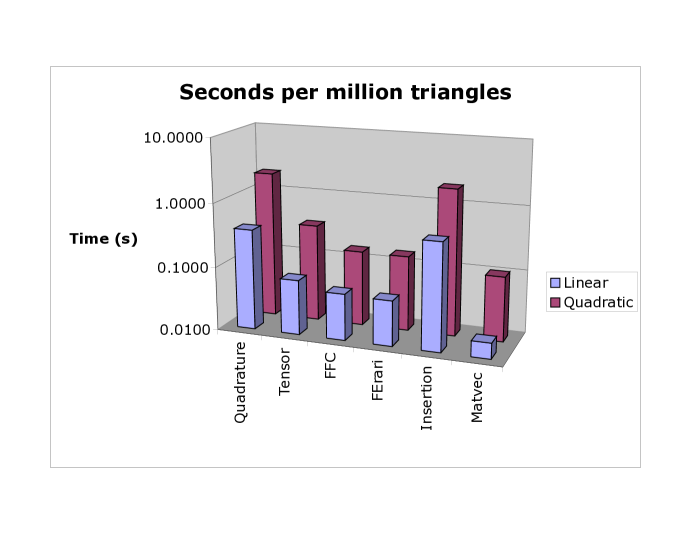
Fig. 2: Seconds to process one million triangles: local stiffness matrices, global matrix insertion, and matrix-vector product

We may draw several conclusions from this. First, precomputing the reference tensors leads to a large performance gain over numerical quadrature. Beyond this, additional benefits are included by omitting the zeros, and more still by doing the FErari optimizations. We seem to have optimized the local computation to the point where it is constrained by read-write to cache rather than by floating point optimization. Second, these optimizations reveal a new bottleneck: matrix insertion. This motivates studying whether we may improve the performance of insertion into the global sparse matrix or else implementing matrix-free methods.

While the FErari optimizations are highly successful for building the matrices, there is still quite a bit of solver overhead to contend with. We used GMRES (boundary conditions were imposed in a way that broke symmetry) preconditioned by the BoomerAMG method of HYPRE [9]. For both linear and quadratics, the Krylov solver converged with only three iterations. However, the cost of building and applying the AMG preconditioner is very large. Using numerical quadrature, building local stiffness matrices accounted for between five and nine percent of the total run time (building the local to global mapping, computing geometry tensors, computing local stiffness matrices, sorting and inserting local matrices into the global matrix, creating and applying the AMG preconditioner, and the rest of the Krylov solver). Keeping everything else constant and switching to the FErari optimized code, building local stiffness matrices took less than one percent of total time. Geometric multigrid algorithms tend to be much more efficient, and we conjecture that the cost of building local matrices would be even more important in this case.

8 Conclusions

The determination of local element matrices involves a novel problem in computational complexity. There is a mapping from (small) geometry matrices to “difference stencils” that must be computed. We have demonstrated the potential speed-up available with simple low-order methods. We have suggested by examples that it may be possible to automate this to some degree by solving abstract graph optimization problems.

9 Acknowledgements

We thank the FEniCS team, and Todd Dupont, Johan Hoffman, and Claes Johnson in particular, for substantial suggestions regarding this paper.

References

- [1] A. A. Albrecht, P. Gottschling, and U. Naumann, Markowitz-type heuristics for computing jacobian matrices efficiently, in International Conference on Computational Science, 2003, pp. 575–584.
- [2] D. N. Arnold, D. Boffi, and R. S. Falk, Quadrilateral h(div) finite elements, SIAM Journal on Numerical Analysis, to appear (2004), pp. 1–2.
- [3] S. Balay, K. Buschelman, V. Eijkhout, W. D. Gropp, D. Kaushik, M. G. Knepley, L. C. McInnes, B. F. Smith, and H. Zhang, PETSc users manual, Tech. Report ANL-95/11 - Revision 2.1.5, Argonne National Laboratory, 2004.
- [4] S. C. Brenner and L. R. Scott, The Mathematical Theory of Finite Element Methods, 2nd Edition, Springer-Verlag, 2002.
- [5] K. A. Cliffe and S. J. Tavener, Implementation of extended systems using symbolic algebra, in Continuation Methods in Fluid Dynamics, D. Henry and A. Bergeon, eds., Notes on Numerical Fluid Mechanics 74, Vieweg, 2000, pp. 81–92.
- [6] M. Crouzeix and P.-A. Raviart, Conforming and nonconforming finite element methods for solving the stationary Stokes equations. I, Rev. Française Automat. Informat. Recherche Opérationnelle Sér. Rouge, 7 (1973), pp. 33–75.
- [7] J. A. Gunnels, F. G. Gustavson, G. M. Henry, and R. A. van de Geijn, FLAME: Formal linear algebra methods environment, Trans. on Math. Software, 27 (2001), pp. 422–455.
- [8] P. Hansbo and A. Szepessy, A velocity-pressure streamline diffusion finite element method for the incompressible Navier-Stokes equations, Comput. Methods Appl. Mech. Engrg., 84 (1990), pp. 175–192.
- [9] V. Henson and U. Yang, BoomerAMG: a Parallel Algebraic Multigrid Solver and Preconditioner, Applied Numerical Mathematics, 41 (2002), pp. 155–177.
- [10] J. Hoffman and A. Logg, DOLFIN: Dynamic Object oriented Library for FINite element computation, Tech. Report 2002–06, Chalmers Finite Element Center Preprint Series, 2002. http://www.fenics.org/dolfin.
- [11] T. J. R. Hughes, L. P. Franca, and M. Balestra, A new finite element formulation for computational fluid dynamics. V. Circumventing the Babuška-Brezzi condition: a stable Petrov-Galerkin formulation of the Stokes problem accommodating equal-order interpolations, Comput. Methods Appl. Mech. Engrg., 59 (1986), pp. 85–99.
- [12] E.-J. Im and K. A. Yelick, Optimizing sparse matrix computations for register reuse in SPARSITY, in Proceedings of the International Conference on Computational Science, vol. 2073 of LNCS, San Francisco, CA, May 2001, Springer, pp. 127–136.
- [13] E.-J. Im, K. A. Yelick, and R. Vuduc, SPARSITY: Framework for optimizing sparse matrix-vector multiply, International Journal of High Performance Computing Applications, 18 (2004). (to appear).
- [14] H. Juarez, L. R. Scott, R. Metcalfe, and B. Bagheri, Direct simulation of freely rotating cylinders in viscous flows by high–order finite element methods, Computers & Fluids, 29 (2000), pp. 547–582.
- [15] R. C. Kirby, Algorithm 839:FIAT, a new paradigm for computing finite element basis functions, ACM Trans. Math. Software, 30 (2004), pp. 502–516.
- [16] R. C. Kirby, M. Knepley, and L. Scott, Evaluation of the action of finite element operators. submitted to BIT.
- [17] D. E. Knuth, The Art of Computer Programming, Volume 2: Seminumerical Algorithms, Third Edition, Reading, Massachusetts: Addison-Wesley, 1997.
- [18] A. N. Laboratory, Petsc 3 web page. http://www-unix.mcs.anl.gov/petsc/petsc-3/.
- [19] A. Logg, FFC: the FEniCS Form Compiler. http://www.fenics.org/ffc.
- [20] K. Long, Sundance, a rapid prototyping tool for parallel PDE-constrained optimization, in Large-Scale PDE-Constrained Optimization, Lecture notes in computational science and engineering, Springer-Verlag, 2003.
- [21] , Sundance home page. http://csmr.ca.sandia.gov/~krlong/sundance.html, 2003.
- [22] R. Vuduc, J. Demmel, and J. Bilmes, Statistical models for automatic performance tuning, International Journal of High Performance Computing Applications, 18 (2004). (to appear).
- [23] R. Vuduc, J. W. Demmel, K. A. Yelick, S. Kamil, R. Nishtala, and B. Lee, Performance optimizations and bounds for sparse matrix-vector multiply, in Proceedings of Supercomputing, Baltimore, MD, USA, November 2002.
- [24] R. Vuduc, A. Gyulassy, J. W. Demmel, and K. A. Yelick, Memory hierarchy optimizations and bounds for sparse , in Proceedings of the ICCS Workshop on Parallel Linear Algebra, P. M. A. Sloot, D. Abramson, A. V. Bogdanov, J. J. Dongarra, A. Y. Zomaya, and Y. E. Gorbachev, eds., vol. LNCS 2660, Melbourne, Australia, June 2003, Springer, pp. 705–714.
- [25] R. Vuduc, S. Kamil, J. Hsu, R. Nishtala, J. W. Demmel, and K. A. Yelick, Automatic performance tuning and analysis of sparse triangular solve, in ICS 2002: Workshop on Performance Optimization via High-Level Languages and Libraries, New York, USA, June 2002.
- [26] R. C. Whaley, A. Petitet, and J. J. Dongarra, Automated empirical optimization of software and the ATLAS project, Parallel Computing, 27 (2001), pp. 3–35. Also available as University of Tennessee LAPACK Working Note #147, UT-CS-00-448, 2000 (www.netlib.org/lapack/lawns/lawn147.ps).