Faraday rotation in bilayer and trilayer graphene in the quantum Hall regime

Abstract

Optical Hall conductivity, as directly related to Faraday rotation, is theoretically studied for bilayer and trilayer graphene. In bilayer graphene, the trigonal warping of the band dispersion greatly affects the resonance structures in Faraday rotation not only in the low-energy region where small Dirac cones emerge, but also in the higher-energy parabolic bands as a sequence of satellite resonances. In ABA-stacked trilayer, the resonance spectrum is a superposition of effective monolayer and bilayer contributions with band gaps, while ABC trilayer exhibits a distinct spectrum peculiar to the cubic-dispersed bands with a strong trigonal warping, where the signals associated with low-energy Dirac cones should be directly observable owing to a large Lifshitz transition energy ($\sim 10\mbox{ meV}$).

I Introduction

The observation of the anomalous quantization of $\sigma_{xy}=\frac{4e^{2}}{h}(n+\frac{1}{2})$ in graphene quantum Hall system has established the existence of massless Dirac-quasiparticle in grapheneNovoselov et al. (2005); Zhang et al. (2005), and kicked off an increasing fascination with the massless Dirac physics of graphene. Optical properties have also been studied, where a point of interest is an unusual optical selection rule. Specifically, the optical Hall conductivity $\sigma_{xy}(\omega)$ is an interesting quantity to look at, since it is an ac-extension of the Hall conductivity which has a topological nature.

The optical Hall conductivity has been theoretically studied for graphene Gusynin et al. (2007); Morimoto et al. (2009); Fialkovsky and Vassilevich (2009), graphite Falkovsky (2011) and topological insulatorsTse and MacDonald (2010). Experimentally, the optical Hall conductivity is measurable through Faraday rotation, since the Faraday rotation angle $\Theta_{H}$ is proportional to $\sigma_{xy}(\omega)$ in quantum Hall regime [where $(n_{0}+n_{s})\gg|\sigma_{xx}(\omega)\pm\sigma_{xy}(\omega)|/(c\epsilon_{0})$] as

$$\Theta_{H}\simeq\frac{1}{(n_{0}+n_{s})c\varepsilon_{0}}\mbox{Re}\,\sigma_{xy}(\omega),$$ (1)

where $n_{0}(n_{s})$ is the refractive index of the air (substrate)O’Connell and Wallace (1982), $c$ the velocity of light, and $\varepsilon_{0}$ the dielectric constant of vacuum. Faraday rotation experimentally starts to be measured both for 2DEG Ikebe et al. (2010) and for graphene Crassee et al. (2011) in the quantum Hall regime. Due to the Dirac nature of quasiparticles in graphene, the optical Hall conductivity in graphene reflects the Dirac Landau level (LL) structure ($\varepsilon_{n}={\rm sgn}(n)\sqrt{n}\hbar\omega_{c}$) and an unusual selection rule ($|n|\leftrightarrow|n|+1$), with Landau index $n$.

Studies so far have focused on the optical Hall conductivity in monolayer graphene quantum Hall system. In the physics of graphene, there are growing interests in bilayer and trilayer graphene systems, since their electronic structures are distinct from that of monolayer graphene. For bilayer graphene the interlayer coupling between the two graphene sheets ($\gamma_{1}$ in Fig.1) changes the monolayer’s Dirac cone into two parabolic bands touching at the K+ and K- points in the Brillouin zone. Novoselov et al. (2006); McCann and Fal fko (2006) To be more precise, if we take account of the second-neighbor interlayer hopping ($\gamma_{3}$ in Fig.1) a trigonal warping is induced on the band dispersion (Fig.1(b)). There, the parabolic bands touching at the Dirac points are reformed into four Dirac cones in the low-energy region. These are connected to the parabolic bands at a higher energy, at which a Lifshitz transition in the topology of Fermi surface takes place.

It is then an interesting question to ask how these will affect optical responses. While the optical longitudinal conductivity $\sigma_{xx}(\omega)$ is discussed in Abergel and Fal’ko (2007); Nicol and Carbotte (2008), and experimentally utilized for determining the band structure Zhang et al. (2008); Li et al. (2009), we propose here that the optical Hall conductivity $\sigma_{xy}(\omega)$ should be a good probe for multi-layer graphene in the quantum Hall regime. Trilayer graphene, the next in the series of multilayer graphene, harbors another interest, since it comes with two different stacking orders, ABA and ABC. The low-energy dispersion of ABA trilayer consists of a monolayer-like Dirac cone and a bilayer-like parabolic bands, which are gapped due to the absence of inversion symmetry in the lattice structure. Guinea et al. (2006); Latil and Henrard (2006); Partoens and Peeters (2006); Lu et al. (2006a); Aoki and Amawashi (2007); Koshino and Ando (2007, 2008); Koshino and McCann (2009a); Koshino and Ando (2009); Koshino and McCann (2011); Sena et al. (2011); Taychatanapat et al. (2011) On the other hand, ABC trilayer has a pair of cubic-dispersed bands with a larger trigonal warping effect than in bilayer graphene, Guinea et al. (2006); Latil and Henrard (2006); Lu et al. (2006b); Aoki and Amawashi (2007); Koshino and McCann (2009b); Zhang et al. (2010) for which LL splitting due to Lifshitz transition is reported Bao et al. (2011). Thus the interest for trilayer is how the stacking dependence appears in the optical Hall conductivity.

These have motivated us to study in this paper the optical (Hall as well as longitudinal) conductivities in bilayer and trilayer graphene systems. We shall show for bilayer graphene that the Lifshitz transition accompanied by the trigonal warping greatly affects the resonance structures in Faraday rotation not only on low-energy scale where Dirac cones emerges but also in the higher-energy range with parabolic bands as a sequence of satellite resonances, whose weight can become large in the vicinity of the Lifshitz transition, hence should be experimentally measurable. Thus, while it would be difficult to directly observe the Lifshitz transition and low-energy Dirac cones due to the tiny energy scale of the trigonal warping ($\sim 1\mbox{ meV}$) , the optical conductivities should provide an experimentally accessible way to detect the trigonal warping as additional resonance structure.

For trilayer graphene, on the other hand, we shall show that the optical conductivities are significantly affected by the difference in the stacking order. In ABA trilayer, the resonance spectrum is a superposition of effective monolayer and bilayer contributions with band gap, while ABC trilayer exhibits a distinct spectrum peculiar to the cubic-dispersed bands. In the latter, the trigonal warping effect is strong with a larger Lifshitz transition energy ($\sim 10\mbox{ meV}$), so that we predict here the signals associated with low-energy Dirac cones should be directly observable.

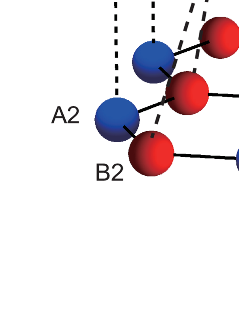
Figure 1: (a) Lattice structure of bilayer graphene with A/B sublattice carbons indicated in blue/red. The unit cell consists of $A_{1}$ and $B_{1}$ carbon atoms in the top layer and $A_{2}$ and $B_{2}$ carbon atoms in the bottom. $\gamma_{0}$: the nearest-neighbor ($A_{1}\leftrightarrow B_{1},A_{2}\leftrightarrow B_{2}$) hopping within each layer, $\gamma_{1}$: the vertical ($B_{1}\leftrightarrow A_{2}$) interlayer hopping, and $\gamma_{3}$: an oblique ($A_{1}\leftrightarrow B_{2}$) interlayer hopping. Two layers are separated by $d=0.334$ nm. (b) Low-energy band dispersion of bilayer graphene with the trigonal warping effect with a Lifshitz transition where the topology of Fermi surface changes from four Dirac cones to one, trigonally warped parabolic dispersion.

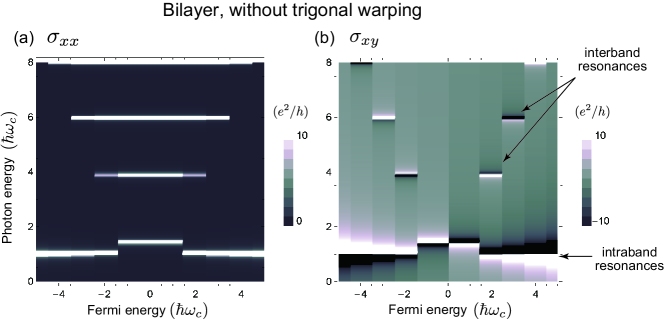
Figure 2: For bilayer graphene QHE system without the trigonal warping effect ($v_{3}=0$), we show (a) the optical longitudinal conductivity $\sigma_{xx}(\epsilon_{F},\omega)$, and (b) optical Hall conductivity $\sigma_{xy}(\epsilon_{F},\omega)$, grey-scale plotted against the Fermi energy $\epsilon_{F}$ and the frequency $\omega$.

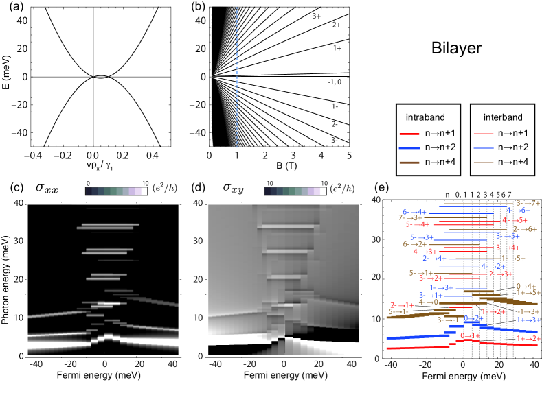
Figure 3: (a) Low-energy band structure, and (b) Landau levels against magnetic field for bilayer graphene with the trigonal warping included. (c) The longitudinal $\sigma_{xx}(\epsilon_{F},\omega)$ and (d) Hall $\sigma_{xy}(\epsilon_{F},\omega)$ gre-scale plotted against the Fermi energy $\epsilon_{F}$ and the frequency $\omega$ for a magnetic field $B=1T$ (a vertical dashed line in (b)). (e) A diagram indicating allowed resonances in $\sigma_{xy}$. Vertical dotted lines indicate the Landau levels. Note that ”-1” (n=-1) and ”1-” (n=1, s=-1)” are different.

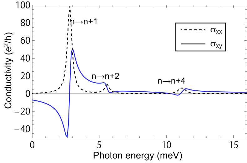
Figure 4: Optical longitudinal ($\sigma_{xx}$; dashed line) and Hall ($\sigma_{xy}$; solid line) conductivities plotted against the frequency $\omega$ for a magnetic field $B=1T$ and the Fermi energy $\epsilon_{F}=-20$ meV.

II Bilayer graphene and trigonal warping

II.1 Effective Hamiltonian

AB-stacked bilayer graphene comprises two graphene sheets coupled by interlayer hoppings as shown in Fig.1, where B sublattice in the top sheet is located just above A sublattice of the bottom sheet (Bernal stacking). A unit cell thus contains four carbon atoms, i.e., A1 and B1 in the top layer and A2 and B2 in the bottom. Hoppings are the nearest-neighbor hopping within each layer ($\gamma_{0}$), the vertical interlayer hopping between B1 and A2 ($\gamma_{1}$). An oblique interlayer hopping between A1 and B2 ($\gamma_{3}$) causes the trigonal warping of the band dispersion. The magnitudes of these are estimated in Ref.Charlier et al. (1991); Dresselhaus and Dresselhaus (2002) as $\gamma_{0}=3.2$ eV, $\gamma_{1}=0.39$ eV, $\gamma_{3}=0.32$ eV. We shall adopt these values hereafter. There is another interlayer hopping parameters, $\gamma_{4}=0.044$ eV, connecting A1 (B1) and A2 (B2), which introduces a small electron-hole asymmetry to the band structure. McClure (1957, 1960)

In a basis with components, $\psi_{A1},\psi_{B1},\psi_{A2},\psi_{B2}$, on the four sites, the Hamiltonian for the bilayer graphene is given as McCann and Fal fko (2006); Guinea et al. (2006); Koshino and Ando (2006)

$$H_{\rm AB}=\begin{pmatrix}0&v\pi^{\dagger}&-v_{4}\pi^{\dagger}&v_{3}\pi\\ v\pi&0&\gamma_{1}&-v_{4}\pi^{\dagger}\\ -v_{4}\pi&\gamma_{1}&0&v\pi^{\dagger}\\ v_{3}\pi^{\dagger}&-v_{4}\pi&v\pi&0\\ \end{pmatrix},$$ (2)

where $\pi=\xi\pi_{x}+i\pi_{y}$, $\pi^{\dagger}=\xi\pi_{x}-i\pi_{y}$, $\mbox{\boldmath$\pi$}=\mbox{\boldmath$p$}+e\mbox{\boldmath$A$}$, with $A$ being the vector potential arising from the applied magnetic field, and the valley index $\xi=\pm 1$ for $K_{\pm}$ points. Here $v=\sqrt{3}a\gamma_{0}/(2\hbar)$ is the band velocity for monolayer graphene, $a\approx 0.246$ nm the distance between the nearest $A$ sites, and $v_{3}=\sqrt{3}a\gamma_{3}/(2\hbar)$, $v_{4}=\sqrt{3}a\gamma_{4}/(2\hbar)$ velocities related to $\gamma_{3}$, $\gamma_{4}$.

The low-energy physics of bilayer graphene for a region where the eigenenergy $\varepsilon$ is much smaller than the interlayer hopping $\gamma_{1}$, is captured by a 2 $\times$ 2 Hamiltonian in a basis of A1/B2 carbon sites, with a perturbation with respect to $\varepsilon/\gamma_{1}$, which is valid for energy scale $|\varepsilon|\ll\gamma_{1}=0.39eV$, as McCann and Fal fko (2006); Koshino and Ando (2006); Koshino and McCann (2011)

$$H^{\rm(eff)}_{\rm AB}=\frac{1}{2m}\begin{pmatrix}0&(\pi^{\dagger})^{2}\\ \pi^{2}&0\end{pmatrix}+v_{3}\begin{pmatrix}0&\pi\\ \pi^{\dagger}&0\end{pmatrix}+\frac{2vv_{4}}{\gamma_{1}}\begin{pmatrix}\pi^{\dagger}\pi&0\\ 0&\pi\pi^{\dagger}\end{pmatrix},$$ (3)

with an effective mass $m=\gamma_{1}/(2v^{2})$. In the absence of magnetic fields, the first term on the right-hand side gives a pair of parabolic bands $E=\pm p^{2}/(2m)$, while the second term coming from $\gamma_{3}$ causes the trigonal warping in the band dispersion, and the third term from $v_{4}$ produces a weak electron-hole asymmetry by adding the band energy $2vv_{4}p^{2}/\gamma_{1}$ in both conduction and valence bands. In the low-energy region, two touching parabolae are reformed into four Dirac cones as shown in Fig.1(b), where the Lifshitz transition (separation of the Fermi surface) occurs at

$$E_{\rm{Lifshitz}}=\frac{1}{2}mv_{3}^{2}\sim 1\,\mbox{meV}.$$ (4)

The Landau level spectrum in a uniform magnetic field $\mbox{\boldmath$B$}={\rm rot}\mbox{\boldmath$A$}$ may be found with the relation $(\pi,\pi^{\dagger})=(\sqrt{2}\hbar/\ell)(a^{\dagger},a)$ for $K_{+}$, or $(\pi,\pi^{\dagger})=(\sqrt{2}\hbar/\ell)(a,a^{\dagger})$ for $K_{-}$. Here $a^{\dagger}$ and $a$ are raising and lowering operators, respectively, which operate on the Landau-level wave function $\phi_{n}$ as $a\phi_{n}=\sqrt{n}\phi_{n-1},a^{\dagger}\phi_{n}=\sqrt{n+1}\phi_{n+1}$, while $\ell=\sqrt{\hbar/(eB)}$ is the magnetic length. If we neglect the $v_{3}$ and $v_{4}$ terms in Eqn.3, the eigenenergies are given byMcCann and Fal fko (2006)

$$\varepsilon_{n,s}=s\hbar\omega_{c}\sqrt{n(n+1)},$$ (5)

where states are labeled by the Landau index $n=-1,0,1,\cdots$, and the band index $s=\pm$ (defined for $n\geq 1$) labeling the conduction ($s=+$) and valence ($s=-$) bands. The cyclotron frequency $\omega_{c}$ is the same as defined for a two-dimensional electron gas (2DEG),

$$\hbar\omega_{c} = \frac{\hbar eB}{m}\simeq 3.5\left(\frac{B}{1T}\right)\mbox{ meV}.$$ (6)

Two zero-energy Landau levels (LLs) appear ($n=0,-1$) at each valley, while for large values of $n$ the LLs tend to be proportional to $n$ as in a 2DEG. The associated eigenstates for $K_{+}$ point are

$$\psi_{n,s}=C_{n}\begin{pmatrix}\phi_{n-1}\\ s\phi_{n+1}\\ \end{pmatrix},$$

$$C_{n}=\left\{\begin{array}[]{cc}1&(n\leq 0)\\ 1/\sqrt{2}&(n\geq 1)\end{array}\right.,$$ (9)

where we defined $\phi_{n}=0$ for $n<0$. The wavefunction at $K_{-}$ is obtained by interchanging the first and second components in Eqn.9.

The $v_{3}$ term in Eqn. 3 causes a hybridization between Landau states $\psi_{n,s}$ and $\psi_{n+3m,s^{\prime}}$, while $v_{4}$ contributes to the energy shift of the Landau levels. The energies and eigenfunctions for high-energy Landau levels with $|E|\gg E_{\rm Lifshitz}$ in $\hbar\omega_{c}\gg\hbar v_{3}/\ell$ ($B>1$T), are expressed in a lowest-order perturbation in $v_{3}$ and $v_{4}$ as

$$\tilde{\varepsilon}_{n,s}\simeq\varepsilon_{n,s}+\frac{2vv_{4}}{\gamma_{1}}\left(n+\frac{1}{2}\right),$$ (10)

$$\tilde{\psi}_{n,s}\simeq\psi_{n,s}+\sum_{s^{\prime}=\pm}\frac{\hbar v_{3}}{\sqrt{2}\ell}\left(\frac{s^{\prime}\sqrt{n-1}\psi_{n-3,s^{\prime}}}{\varepsilon_{n,s}-\varepsilon_{n-3,s^{\prime}}}+\right.$$

$$\qquad\qquad\qquad\qquad\left.\frac{s\sqrt{n+2}\psi_{n+3,s^{\prime}}}{\varepsilon_{n,s}-\varepsilon_{n+3,s^{\prime}}}\right).$$ (11)

In the low-energy region, $|E|<E_{\rm Lifshitz}$, on the other hand, the spectrum is reconstructed into monolayer-like Landau levels as $\varepsilon_{N}={\rm sgn}(N)\sqrt{3N}\hbar\omega_{\rm{trig}}$ for the center cone and $\varepsilon_{N}={\rm sgn}(N)\sqrt{N}\hbar\omega_{\rm{trig}}$ for three off-center cones McCann and Fal fko (2006), where

$$\hbar\omega_{\rm{trig}}=v_{3}\sqrt{2\hbar eB}\simeq 3.7\sqrt{\frac{B}{1{\rm T}}}\mbox{ meV}.$$ (12)

The first excited level $N=1$ in this series appears in small enough magnetic fields such that $\hbar\omega_{\rm trig}<E_{\rm Lifshitz}$, which amounts to $B<0.08$T.

II.2 Optical selection rules

The optical longitudinal ($\sigma_{xx}(\omega)$) and Hall ($\sigma_{xy}(\omega)$) conductivities are evaluated from the Kubo formula as

$$\sigma_{\alpha\beta}(\omega)=\frac{\hbar}{iL^{2}}\sum_{ab}j_{\alpha}^{ab}j_{\beta}^{ba}\frac{f(\epsilon_{b})-f(\epsilon_{a})}{\epsilon_{b}-\epsilon_{a}}\frac{1}{\epsilon_{b}-\epsilon_{a}-\hbar\omega-i\eta},$$ (13)

where $f(\varepsilon)$ is the Fermi distribution, $\epsilon_{a}$ the energy of the eigenstate $|a\rangle$, $j_{\alpha}^{ab}=\langle a|j_{\alpha}|b\rangle$ the matrix element of the current operator $\mbox{\boldmath$j$}=\partial H/\partial\mbox{\boldmath$A$}$, and $\eta$ a small energy cutoff for a stability of the calculation which we set to 0.1 meV.

In multilayer graphene the optical selection rule is of crucial interest, which just reflects the current matrices, $j_{x}^{ab}j_{y}^{ba}$, appearing in the Kubo formula. Let us consider in the effective $2\times 2$ Hamiltonian Eqn.3, for which the current matrices read

$$j_{x} = \frac{\xi}{m}\begin{pmatrix}0&\pi^{\dagger}\\ \pi&0\end{pmatrix}+\xi v_{3}\begin{pmatrix}0&1\\ 1&0\end{pmatrix}+\frac{2vv_{4}}{\gamma_{1}}\begin{pmatrix}2\pi_{x}&0\\ 0&2\pi_{x}\end{pmatrix},$$

$$j_{y} = \frac{1}{m}\begin{pmatrix}0&-i\pi^{\dagger}\\ i\pi&0\end{pmatrix}+v_{3}\begin{pmatrix}0&i\\ -i&0\end{pmatrix}+\frac{2vv_{4}}{\gamma_{1}}\begin{pmatrix}2\pi_{y}&0\\ 0&2\pi_{y}\end{pmatrix}.$$

The first term on the right-hand side of each equation is responsible for $n\leftrightarrow n\pm 1$ transitions. When we express $a=(n,s)$ and $b=(n+1,s^{\prime})$ in the Kubo formula (Eqn.13), the corresponding contribution is

$$j_{x}^{n,n+1}j_{y}^{n+1,n}=-i(C_{n}C_{n+1})^{2}\frac{2\hbar^{2}}{m^{2}\ell^{2}}(n+1),$$ (15)

where we have dropped the band indeces $s,s^{\prime}$, since it is independent of their combination.

In addition, the second term in the current operators in Eqn. LABEL:eq_current_operators, and also the hybridization between $n$ and $n+3m$ in the eigenstates Abergel and Fal’ko (2007), give rise to additional transition series,

$$n\leftrightarrow n+1+3m,$$ (16)

$$n\leftrightarrow n+2+3m,$$ (17)

with all the combinations of $s$ and $s^{\prime}$. A similar selection rule was previously found for graphite Falkovsky (2011); Orlita et al. (2012). In contrast, the third term including $v_{4}$ in Eqn. LABEL:eq_current_operators contributes to the $n\leftrightarrow n\pm 1$ transistions as the first term, so that it does not cause any additional transitions but adds a small correction to Eqn. 15.

For the high-energy Landau levels with $|E|\gg E_{\rm Lifshitz}$, the contribution to $\sigma_{xy}(\omega)$ in the resonances of Eqns. (16) and (17) becomes of the order of $v_{3}^{2m}$ and $v_{3}^{2(m+1)}$, respectively. In the lowest-order perturbation in $v_{3}$, the transitions are respectively allowed for $n\leftrightarrow n+4$ and $n\leftrightarrow n+2$, where the current matrices are respectively given by

$$j_{x}^{n,n+4}j_{y}^{n+4,n}\approx-i\left(\frac{v_{3}}{6}\right)^{2},$$

$$j_{x}^{n,n+2}j_{y}^{n+2,n}\approx i\left(\frac{v_{3}}{6}\right)^{2}.$$ (18)

Since the weights of these additional resonances have no dependence on the Landau index $n$ while the $n\leftrightarrow n+1$ resonance depends linearly on $n$, the resonances arising from the trigonal warping should be relatively prominent in a low Fermi energy ($\epsilon_{F}$) region. We also note that the factor $j_{x}^{ab}j_{y}^{ba}$ may have positive or negative sign depending on the transition sequence. This property is specific to $\sigma_{xy}$, since the corresponding factors in $\sigma_{xx}$ is $|j_{x}^{ab}|^{2}$, which naturally have no information about the sign of the resonances.

II.3 Numerical results

We start with calculating the optical Hall conductivity using Kubo formula Eqn.13 for the bilayer system using the effective Hamiltonian (Eqn.3) without the trigonal warping term. The result for the optical longitudinal and Hall conductivities in Fig.2(a,b) shows that an intra-band transition $(n,s)\leftrightarrow(n+1,s)$ occurs around

$$\hbar\omega_{\rm intra}\sim\hbar\omega_{c}.$$ (19)

This is natural, since LLs are almost equally spaced, unlike in the monolayer case where LL energy $\propto\sqrt{n}$ is not equally separated. On top of this, there are inter-band transitions across the band-touching point, with a selection rule $(n,\pm)\leftrightarrow(n+1,\mp)$. Thus the inter-band transition energy is

$$\hbar\omega_{\rm inter}\simeq 2|\epsilon_{F}|$$ (20)

for large enough $n$.

As stressed above, an important difference between $\sigma_{xx}$ and $\sigma_{xy}$ is that resonance factor $j_{\alpha}^{ab}j_{\beta}^{ba}$ is always positive for $\sigma_{xx}$, while it may have both signs for $\sigma_{xy}$. This puts a clear distinction for inter-band resonances of optical longitudinal and Hall conductivities. For $\sigma_{xx}$, resonances $(n+1,-)\to(n,+)$ and $(n,-)\to(n+1,+)$ add up, and inter-band resonances occur over an entire region of Fermi energy between negative $(n+1,-)$ and positive $(n+1,+)$ LL energies. By contrast, for $\sigma_{xy}$, resonances, $(n+1,-)\to(n,+)$ and $(n,-)\to(n+1,+)$ have opposites signs in the resonance factor, so that they cancel with each other for a region of Fermi energy between $(n,-)$ and $(n,+)$ LLs. So the inter-band resonance for $\sigma_{xy}$ is peaked at $\epsilon_{n+1,-}<\epsilon_{F}<\epsilon_{n,-}$ and $\epsilon_{n,+}<\epsilon_{F}<\epsilon_{n+1,+}$ with opposite signs.

Now we examine the effect of the trigonal warping on the optical responses. We go back to the original $4\times 4$ Hamiltonian (Eqn.2) including all the hopping terms in order to get quantitatively accurate results for all the energy regions. We have diagonalized the Hamiltonian with a basis set spanned by a finite number of Landau functions $\phi_{n}$ ($0\leq n<100$) to calculate the dynamical conductivities with the formula Eqn.13. In Fig.3 we show a result for bilayer graphene in a magnetic field $B=1$T. A behavior of LLs with magnetic fields (Landau fan diagram ) is indicated in Fig.3(b). At $B=1$T, the monolayer-like LLs in low-energy Dirac cones are not seen as the LL spacing already exceeds $E_{\rm Lifshitz}$.

Figures 3(c,d) are $\sigma_{xx}(\epsilon_{F},\omega)$ and $\sigma_{xy}(\epsilon_{F},\omega)$, respectively, plotted against the Fermi energy $\epsilon_{F}$ and the frequency $\omega$. While the result becomes complicated, we can make an identification of the resonance structure in Fig. 3(e), where we have extracted, from the Landau level spectrum (Fig.3(b)) at 1T, the expected positions of allowed resonances, as argued above. There we can actually observe the satellite resonances of $n\leftrightarrow n+2$ and $n\leftrightarrow n+4$, which are absent in purely parabolic bilayer. It should be noted that, even though it is hard to directly observe the Landau levels below the Lifshitz transition due to the tiny $E_{\rm{Lifshitz}}$, the satellite transitions in a region outside of $E_{\rm{Lifshitz}}$ should be observable as a manifestation of the trigonal warping effect.

For $\sigma_{xy}(\omega)$, the weight of the satellite peaks is constant as expected from the current matrices of Eqn. 18, while that for the original peak ($n\leftrightarrow n+1$) depends on the Fermi energy through index $n$, as $j_{x}^{n,n+1}j_{y}^{n+1,n}\simeq-in\hbar^{2}/(2\ell^{2}m^{2})\simeq-i\epsilon_{F}/(2m)$. So the relative weight of satellite to original peak is larger for smaller Landau index $n$ or smaller Fermi energy.

To make the signs of the resonances clearer, Figure 4 plots the optical Hall conductivity $\sigma_{xy}$ against the frequency $\omega$ at a fixed Fermi energy $\epsilon_{F}=20$ meV. We can see that, in addition to a large resonance $n\to n+1$ around $\hbar\omega_{c}=3$ meV, satellite resonances $n\to n+2$ and $n\to n+4$ are seen. In the case of the longitudinal conductivity $\sigma_{xx}$ the resonance appears as a symmetrical peak, while a resonance in $\sigma_{xy}$ has an odd structure around a resonance frequency $\omega_{c}$. Thus the sign in the resonance weight for $\sigma_{xy}$ determines the resonance shape, i.e., in accordance with the sign of $j_{x}^{ab}j_{y}^{ba}/i$ in Eqs. 15 and 18, the resonance asymmetry of $n\to n+2$ is opposite to those of $n\to n+1$ and $n\to n+4$. These features can be utilized for an experimental identification of resonances in the Faraday rotation, which is directly proportional to $\sigma_{xy}(\omega)$ with Eqn.1, where the unit $e^{2}/h$ in $\sigma_{xy}(\omega)$ is related to $2\alpha/(n_{0}+n_{s})$ rad in Faraday rotation with the fine structure constant $\alpha\simeq 1/137$.

The resonance frequency for intra-band transition within the conduction band is larger than those within the valence band, which is a consequence of an electron-hole asymmetry due to $\gamma_{4}$ term. A deviation in the cyclotron mass for electron and hole bands prevents a complete cancellation between $(n,-)\to(n+1,+)$ and $(n+1,-)\to(n,+)$ transitions, which result in small interband transitions in a wide region of Fermi energy.

III Trilayer graphene

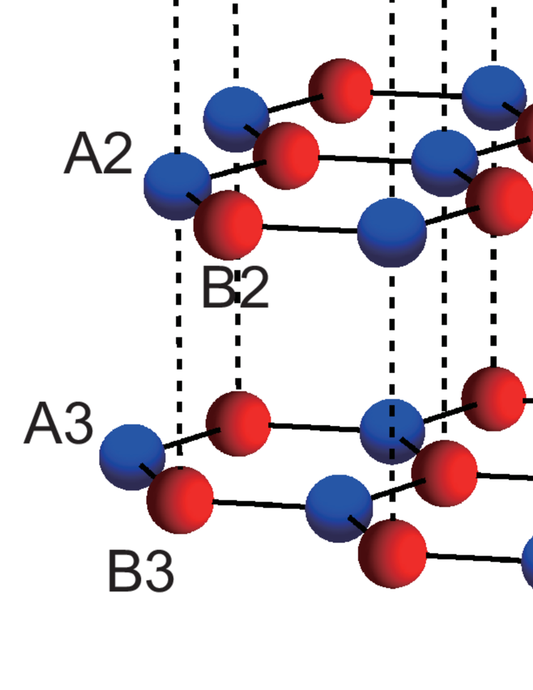
Figure 5: Lattice structure of trilayer graphene with (a) ABA stacking and (b) ABC stacking.

Now let us move on to optical responses of trilayer graphene QHE systems. Trilayer graphene occurs in two different stacking orders, i.e., ABA and ABC stacking orders as shown in Fig.5. In both ABA and ABC trilayers, the spatial arrangement of the two successive layers is the similar to bilayer graphene, while the relation between the first and third layers is different between two. The variation in the stacking order results in totally different electronic structures, and here we show that this can be dramatically reflected in optical responses.

III.1 ABA-stacked trilayer

For ABA stacked trilayer, the effective Hamiltonian around $K_{+}$/$K_{-}$ points is given by a $6\times 6$ matrix (the dimension being 2 sublattices $\times$ 3 layers) as Guinea et al. (2006); Partoens and Peeters (2006); Lu et al. (2006a); Koshino and Ando (2007)

$$H_{\rm ABA}=\begin{pmatrix}0&v\pi^{\dagger}&-v_{4}\pi^{\dagger}&v_{3}\pi&\gamma_{2}/2&0\\ v\pi&\Delta^{\prime}&\gamma_{1}&-v_{4}\pi^{\dagger}&0&\gamma_{5}/2\\ -v_{4}\pi&\gamma_{1}&\Delta^{\prime}&v\pi^{\dagger}&-v_{4}\pi&\gamma_{1}\\ v_{3}\pi^{\dagger}&-v_{4}\pi&v\pi&0&v_{3}\pi^{\dagger}&-v_{4}\pi\\ \gamma_{2}/2&0&-v_{4}\pi^{\dagger}&v_{3}\pi&0&v\pi^{\dagger}\\ 0&\gamma_{5}/2&\gamma_{1}&-v_{4}\pi^{\dagger}&v\pi&\Delta^{\prime}\end{pmatrix},$$ (21)

where $\gamma_{0}$, $\gamma_{1}$ and $\gamma_{3}$ are the same hopping parameters as in bilayer, $\Delta^{\prime}$ the on-site energy difference between the atoms with and without vertical bond $\gamma_{1}$, and $\gamma_{2}(\gamma_{5})$ the next-nearest interlayer hoppings between $A1$ and $A3$ ($B1$ and $B3$). We adopt the values for bulk graphite, $\gamma_{2}$=-0.020eV, $\gamma_{5}$=0.038eV, $\Delta^{\prime}$=0.050eV. Charlier et al. (1991); Dresselhaus and Dresselhaus (2002)

With a unitary transformation Koshino and Ando (2007, 2008); Koshino and McCann (2009a); Koshino and Ando (2009); Koshino and McCann (2011), this Hamiltonian is decomposed into two blocks as

$$\tilde{H}_{\rm ABA}=\begin{pmatrix}H_{m}&0\\ 0&H_{b}\\ \end{pmatrix}.$$ (22)

The first 2 by 2 block,

$$H_{m}=\begin{pmatrix}-\gamma_{2}/2&v\pi^{\dagger}\\ v\pi&-\gamma_{5}/2+\Delta^{\prime}\\ \end{pmatrix},$$ (23)

corresponds to a massive Dirac Hamiltonian with a shift in Fermi energy, while the other 4 by 4 block,

$$H_{b}=\begin{pmatrix}\gamma_{2}/2&v\pi^{\dagger}&-\sqrt{2}v_{4}\pi^{\dagger}&\sqrt{2}v_{3}\pi\\ v\pi&\gamma_{5}/2+\Delta^{\prime}&\sqrt{2}\gamma_{1}&-\sqrt{2}v_{4}\pi^{\dagger}\\ -\sqrt{2}v_{4}\pi&\sqrt{2}\gamma_{1}&\Delta^{\prime}&v\pi^{\dagger}\\ \sqrt{2}v_{3}\pi^{\dagger}&-\sqrt{2}v_{4}\pi&v\pi&0\\ \end{pmatrix},$$ (24)

corresponds to a gapped bilayer Hamiltonian with another shift in energy. So the low-energy physics of ABA stacked trilayer graphene is effectively described as a superposition of gapped monolayer and gapped bilayer band contributions as seen in the low-energy band structure in Fig.6(a).

In Fig.6(b), LLs are plotted with magnetic field B, which are labeled with M (B) for monolayer (bilayer) blocks, Landau index $n$, and band index $\pm$ (for $n\geq 1$). For moderate magnetic fields $B\sim 1$ T, the Landau level spacing $\propto\sqrt{B}$ for monolayer is much larger than that for bilayer $\propto B$. Since bands are gapped, zero-energy LLs of monolayer and bilayer appear at the bottom (top) of the conduction (valence) bands for $K_{+}$ ($K_{-}$) valley.

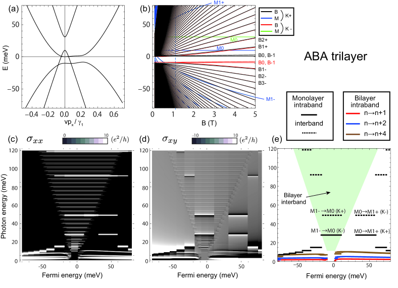
Figure 6: (a) Low-energy band structure, and (b) Landau levels against magnetic field for ABA-stacked trilayer graphene. (c) Longitudinal $\sigma_{xx}(\epsilon_{F},\omega)$ and (d) Hall $\sigma_{xy}(\epsilon_{F},\omega)$ plotted against the Fermi energy $\epsilon_{F}$ and the frequency $\omega$ for a magnetic field $B=1T$ (a dashed line in (b)). (e) A diagram indicating allowed resonances in $\sigma_{xy}$.

We now look at the result for the optical longitudinal $\sigma_{xx}(\epsilon_{F},\omega)$ and Hall conductivity $\sigma_{xy}(\epsilon_{F},\omega)$ plotted against the Fermi energy $\epsilon_{F}$ and frequency $\omega$ for ABA stacked trilayer graphene QHE system in Figs.6(c,d). We can discern contributions from monolayer-like Dirac LLs and from bilayer LLs, both of which exhibit intra-band and inter-band transitions. Since Dirac cone is massive and M0 LL is situated at the bottom of conduction band for $K_{+}$ valley and the top of valence band for $K_{-}$, so that $M0\to M1+$ resonance occurs at a lower energy than $M1-\to M0$ for $K_{+}$, and vice versa for $K_{-}$ valley. A cancellation of resonances in $\sigma_{xy}$, due to opposite signs in current matrices, occurs between $M1-\to M0$ for $K_{+}$ and $M0\to M1+$ for $K_{-}$ for a region of Fermi energy between $M0(K_{+})$ and $M0(K_{-})$, while this is not the case with $\sigma_{xx}$. For bilayer contributions satellites appear due to the trigonal warping effect as $(n,s)\leftrightarrow(n+1+3m,s^{\prime})$ and $(n,s)\leftrightarrow(n+2+3m,s^{\prime})$ as in optical responses for bilayer graphene (Fig.3).

So the message here is the ac optical responses in the ABA-stacked trilayer graphene accommodates a curious mixture of contributions from an effective massive monolayer and from an effective gapped bilayer with the trigonal warping effect.

III.2 ABC-stacked trilayer

If we turn to ABC stacked bilayer graphene, the effective Hamiltonian around $K$ point is a $6\times 6$ matrix as Guinea et al. (2006); Lu et al. (2006b); Koshino and McCann (2009b)

$$H_{\rm ABC}=\begin{pmatrix}0&v\pi^{\dagger}&-v_{4}\pi^{\dagger}&v_{3}\pi&0&\gamma_{2}/2\\ v\pi&0&\gamma_{1}&-v_{4}\pi^{\dagger}&0&0\\ -v_{4}\pi&\gamma_{1}&0&v\pi^{\dagger}&-v_{4}\pi^{\dagger}&v_{3}\pi\\ v_{3}\pi^{\dagger}&-v_{4}\pi&v\pi&0&\gamma_{1}&-v_{4}\pi^{\dagger}\\ 0&0&-v_{4}\pi&\gamma_{1}&0&v\pi^{\dagger}\\ \gamma_{2}/2&0&v_{3}\pi^{\dagger}&-v_{4}\pi&v\pi&0\end{pmatrix}.$$ (25)

We can derive a low-energy effective Hamiltonian as a $2\times 2$ matrix with basis for A1 and B3, where we eliminate the states coupled by $\gamma_{1}$. As in the case of bilayer, a perturbation in $\varepsilon/\gamma_{1}$ gives the effective Hamiltonian for ABC trilayer graphene as Koshino and McCann (2009b),

$$H^{\rm(eff)}_{\rm ABC}=\frac{v^{3}}{\gamma_{1}^{2}}\begin{pmatrix}0&(\pi^{\dagger})^{3}\\ \pi^{3}&0\end{pmatrix}+\left(\frac{\gamma_{2}}{2}-\frac{2vv_{3}\mbox{\boldmath$\pi$}^{2}}{\gamma_{1}}\right)\begin{pmatrix}0&1\\ 1&0\end{pmatrix},$$ (26)

where $\mbox{\boldmath$\pi$}^{2}=(\pi^{\dagger}\pi+\pi\pi^{\dagger})/2$, and we neglected $v_{4}$ term which gives the electron-hole asymmetry in a similar manner to bilayer graphene. In the absence of magnetic fields, the first term gives a pair of cubic-dispersed bands touching at zero energy, while the second term involving $\gamma_{2}$ and $v_{3}$ causes a trigonal warping in the band dispersion. In a low-energy region, the cubic bands are reformed into three Dirac cones at off center momenta located in $120^{\circ}$ symmetry around $K_{\pm}$ point. The Lifshitz transition occurs at

$$E_{\rm{Lifshitz}}\approx\frac{\gamma_{2}}{2}\sim 10\,\mbox{meV},$$ (27)

which is an order of magnitude greater than in bilayer’s.

If we first neglect $\gamma_{2}$ and $v_{3}$ and consider the cubic part alone in Eqn. 26, LLs areGuinea et al. (2006); Koshino and McCann (2009b)

$$\varepsilon_{n,s}=s\hbar\omega_{\rm{ABC}}\sqrt{n(n+1)(n+2)},$$ (28)

where $n\geq-2$ is the Landau index, $s=\pm$ (only for $n\geq 1$) the band index, and

$$\hbar\omega_{\rm{ABC}}=\frac{v^{3}}{\gamma_{1}^{2}}\left(\frac{\sqrt{2}\hbar}{\ell}\right)^{3}=\frac{v^{3}}{\gamma_{1}^{2}}(2\hbar eB)^{\frac{3}{2}}.$$ (29)

A peculiar magnetic field dependence of cyclotron energy $\propto B^{\frac{3}{2}}$ for ABC trilayer graphene implies a smaller LL spacing compared to the monolayer’s LL $\propto B^{\frac{1}{2}}$ and bilayer’s LL $\propto B$ for weak magnetic fields. The associated wavefunction at $K_{+}$ point is

$$\psi_{n,s}=C_{n}\begin{pmatrix}\phi_{n-1}\\ s\phi_{n+2}\end{pmatrix},$$ (30)

where $C_{n}$ is defined in Eqn. 9. The wavefunction at $K_{-}$ is obtained by interchanging the first and second components in Eqn. 30.

Similar to bilayer, the trigonal warping effect due to $\gamma_{2}$ and $v_{3}$ hybridizes $\psi_{n,s}$ with $\psi_{n+3m,s^{\prime}}$. In the low-energy region $|E|<E_{\rm Lifshitz}$, the spectrum is reconstructed into the monolayer-like Landau levels from small Dirac cones as a series $\varepsilon_{N}={\rm sgn}(N)\sqrt{N}\hbar\omega_{\rm{trig}}$, where

$$\hbar\omega_{\rm{trig}} = 3\left|\frac{\gamma_{2}}{2\gamma_{1}}\right|^{2/3}\left[1+\frac{4v_{3}}{3v}\left(\frac{2\gamma_{1}}{\gamma_{2}}\right)^{1/3}\right]^{1/2}v\sqrt{2\hbar eB}$$ (31)

$$\simeq 10\sqrt{\frac{B}{1{\rm T}}}\mbox{ meV}.$$

Each monolayer-like level is three-fold degenerate reflecting the number of small Dirac cones. For larger magnetic fields the degeneracy of the $N$-th level is lifted when $\varepsilon_{N}$ exceeds $E_{\rm Lifshitz}$, and the three levels eventually connect to $n=3N,3N-1$ and $3N-2$ in the cubic band in Eqn. 28. The first excited level $N=1$ can appear when $\hbar\omega_{\rm trig}<E_{\rm Lifshitz}$ or $B<\sim 1$T, which is much larger than in bilayer graphene.

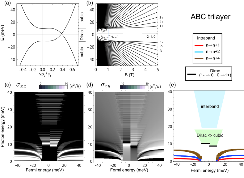
Figure 7: (a) Low-energy band structure, and (b) Landau levels against magnetic field for ABC-stacked trilayer graphene. (c) Longitudinal $\sigma_{xx}(\epsilon_{F},\omega)$ and (d) Hall $\sigma_{xy}(\epsilon_{F},\omega)$ plotted against the Fermi energy $\epsilon_{F}$ and the frequency $\omega$ for a magnetic field $B=1T$ (a dashed line in (b)). (e) A diagram indicating allowed resonances in $\sigma_{xy}$.

Now we go back to the original $6\times 6$ Hamiltonian including all the hopping terms (Eqn.25) to discuss optical conductivities calculated with diagonalization and Kubo formula. In a low-energy region ($\sim$ 10 meV), Dirac cones appear due to trigonal warping effects as seen in the band dispersion (Fig.7(a)). In the LL spectrum in Fig.7(b), a Lifshitz transition is clearly identified at $E_{\rm Lifshitz}=10$meV, which separates Dirac LLs and ABC cubic LLs.

Figures 7(c,d) show the optical longitudinal $\sigma_{xx}(\epsilon_{F},\omega)$ and Hall conductivities $\sigma_{xy}(\epsilon_{F},\omega)$ plotted against the Fermi energy $\epsilon_{F}$ and frequency $\omega$ for ABC stacked trilayer graphene QHE system with $B=1$T. At this particular magnetic field, there are three Landau levels $N=-1,0,1$ inside each Dirac cone, where the $N=\pm 1$ levels are close to the Lifshitz transision. The higher levels are outside of the Dirac cones, and can be regarded to belong to the the cubic dispersion. Accordingly we see cyclotron resonances between $1-\to 0$ and $0\to 1+$ in $E_{F}<E_{\rm Lifshitz}$, while outside we see transitions between cubic LLs $\propto B^{\frac{3}{2}}$ with much smaller level spacings than for Dirac LLs $\propto\sqrt{B}$. In addition to resonances $n\leftrightarrow n+1$, the trigonal warping again gives rise to satellite transitions $n\leftrightarrow n+4$ and $n\leftrightarrow n+2$ with opposite resonance weights. There also emerge small resonances between Dirac $n=0$ LL and cubic LLs across the Lifshitz transition energy. Due to the ABC trilayer LLs arising from the cubic dispersion (Eqn.28) the intra-band transition energies show behaviors $\propto n^{1/2}$ with Landau index $n$, which is different from monolayer ($\propto n^{-1/2}$) or bilayer (constant), while the inter-band transition energies are qualitatively similar to $\sim 2\epsilon_{F}$.

Thus an message in the case of ABC trilayer graphene is that the trigonal warping effect is an order of magnitude enhanced than in bilayer graphene, so it will be experimentally more feasible to access the effects induced by the trigonal warping.

IV Summary

We have studied the optical Hall conductivity for bilayer and trilayer graphene. In bilayer graphene the trigonal warping effect causes a Lifshitz transition with an emergence of four Dirac cones in a small energy scale $\sim 1\mbox{ meV}$. The trigonal warping is shown here to affect optical transitions as additional transitions arising from mixing of LLs whose Landau indices differ by 3 and the opposite sign of resonance weights for transitions $n\leftrightarrow n+2$. For trilayer graphene, which comes with two stacking orders, we have shown that the optical conductivity of ABA in low-energy region comprises contributionf from of monolayer-like massive Dirac and gapped bilayer with an electron-hole asymmetry, while ABC stacking has an order of magnitude larger trigonal warping effect, exhibiting resonances of Dirac LLs inside the Lifshitz transition ($\sim 10$ meV), and a sequence of resonances for the cubic bands with cyclotron energy $\propto B^{\frac{3}{2}}$. This is predicted to be observable.

There are several reports that the electron-electron interaction opens an band gap of a few meV at charge neutrality point in bilayer and trilayer graphene Velasco Jr et al. (2012); Bao et al. (2011). If we consider the effect of the many-body induced gap in the effective models phenomenologically, this would cause a valley splitting of $n=0$ LL and energy shift of resonances associated with low-lying levels, while the transitions associated to high LLs away from the Dirac points, including those of satellite transitions, should not be much affected. We leave the calculation including those effects for future works.

There are various other problems. One is effects of disorder, which in this paper is treated as a phenomenological broadening of the energies, assumed to be small. However, the localization physics is important for understanding the quantum Hall physics, so that it should be interesting to treat disorder more accurately with methods such as diagonalization technique as done in Ref.Morimoto et al. (2010); Morimoto and Aoki (2012), and consider the localization effects on multilayer graphene in the quantum Hall regime. It would be another interesting problem to ask how various types of disorder, chiral-symmetry preserving and non-preserving, affect the optical responses in the multilayer graphene, since it is known that the presence or absence of chiral symmetry greatly affects the behavior of zero energy LLs for the bilayer graphene Kawarabayashi et al. (2012).

References

- Novoselov et al. (2005) K. Novoselov, A. Geim, S. Morozov, D. Jiang, M. Katsnelson, I. Grigorieva, S. Dubonos, and A. Firsov, Nature 438, 197 (2005).
- Zhang et al. (2005) Y. Zhang, Y. W. Tan, H. L. Stormer, and P. Kim, Nature 438, 201 (2005).
- Gusynin et al. (2007) V. P. Gusynin, S. G. Sharapov, and J. P. Carbotte, J. Phys.: Condens. Matter 19, 026222 (2007).
- Morimoto et al. (2009) T. Morimoto, Y. Hatsugai, and H. Aoki, Phys. Rev. Lett. 103, 116803 (2009).
- Fialkovsky and Vassilevich (2009) I. V. Fialkovsky and D. V. Vassilevich, J. Phys. A: Math. Theor. 42, 442001 (2009).
- Falkovsky (2011) L. A. Falkovsky, Phys. Rev. B 84, 115414 (2011).
- Tse and MacDonald (2010) W.-K. Tse and A. H. MacDonald, Phys. Rev. B 82, 161104 (2010).
- O’Connell and Wallace (1982) R. F. O’Connell and G. Wallace, Phys. Rev. B 26, 2231 (1982).
- Ikebe et al. (2010) Y. Ikebe, T. Morimoto, R. Masutomi, T. Okamoto, H. Aoki, and R. Shimano, Phys. Rev. Lett. 104, 256802 (2010).
- Crassee et al. (2011) I. Crassee, J. Levallois, A. Walter, M. Ostler, A. Bostwick, E. Rotenberg, T. Seyller, D. Van Der Marel, and A. Kuzmenko, Nature Physics 7, 48 (2011).
- Novoselov et al. (2006) K. Novoselov, E. McCann, S. Morozov, V. Fal fko, M. Katsnelson, U. Zeitler, D. Jiang, F. Schedin, and A. Geim, Nature Phys. 2, 177 (2006).
- McCann and Fal fko (2006) E. McCann and V. Fal fko, Phys. Rev. Lett. 96, 86805 (2006).
- Abergel and Fal’ko (2007) D. S. L. Abergel and V. I. Fal’ko, Phys. Rev. B 75, 155430 (2007).
- Nicol and Carbotte (2008) E. J. Nicol and J. P. Carbotte, Phys. Rev. B 77, 155409 (2008).
- Zhang et al. (2008) L. M. Zhang, Z. Q. Li, D. N. Basov, M. M. Fogler, Z. Hao, and M. C. Martin, Phys. Rev. B 78, 235408 (2008).
- Li et al. (2009) Z. Q. Li, E. A. Henriksen, Z. Jiang, Z. Hao, M. C. Martin, P. Kim, H. L. Stormer, and D. N. Basov, Phys. Rev. Lett. 102, 037403 (2009).
- Guinea et al. (2006) F. Guinea, A. H. Castro Neto, and N. M. R. Peres, Phys. Rev. B 73, 245426 (2006).
- Latil and Henrard (2006) S. Latil and L. Henrard, Phys. Rev. Lett. 97, 036803 (2006).
- Partoens and Peeters (2006) B. Partoens and F. Peeters, Physical Review B 74, 075404 (2006).
- Lu et al. (2006a) C. Lu, C. Chang, Y. Huang, R. Chen, and M. Lin, Physical Review B 73, 144427 (2006a).
- Aoki and Amawashi (2007) M. Aoki and H. Amawashi, Solid State Commun. 142, 123 (2007).
- Koshino and Ando (2007) M. Koshino and T. Ando, Phys. Rev. B 76, 085425 (2007).
- Koshino and Ando (2008) M. Koshino and T. Ando, Phys. Rev. B 77, 115313 (2008).
- Koshino and McCann (2009a) M. Koshino and E. McCann, Phys. Rev. B 79, 125443 (2009a).
- Koshino and Ando (2009) M. Koshino and T. Ando, Solid State Communications 149, 1123 (2009).
- Koshino and McCann (2011) M. Koshino and E. McCann, Phys. Rev. B 83, 165443 (2011).
- Sena et al. (2011) S. H. R. Sena, J. M. Pereira, F. M. Peeters, and G. A. Farias, Phys. Rev. B 84, 205448 (2011).
- Taychatanapat et al. (2011) T. Taychatanapat, K. Watanabe, T. Taniguchi, and P. Jarillo-Herrero, Nature Phys. 7, 621 (2011).
- Lu et al. (2006b) C. L. Lu, H. C. Lin, C. C. Hwang, J. Wang, M. F. Lin, and C. P. Chang, Appl. Phys. Lett. 89, 221910 (2006b).
- Koshino and McCann (2009b) M. Koshino and E. McCann, Phys. Rev. B 80, 165409 (2009b).
- Zhang et al. (2010) F. Zhang, B. Sahu, H. Min, and A. H. MacDonald, Phys. Rev. B 82, 035409 (2010).
- Bao et al. (2011) W. Bao, L. Jing, J. Velasco Jr, Y. Lee, G. Liu, D. Tran, B. Standley, M. Aykol, S. Cronin, D. Smirnov, et al., Nature Physics 7, 948 (2011).
- Charlier et al. (1991) J. Charlier, X. Gonze, and J. Michenaud, Phys. Rev. B 43, 4579 (1991).
- Dresselhaus and Dresselhaus (2002) M. Dresselhaus and G. Dresselhaus, Advances in Physics 51, 1 (2002).
- McClure (1957) J. W. McClure, Phys. Rev. 108, 612 (1957).
- McClure (1960) J. W. McClure, Phys. Rev. 119, 606 (1960).
- Koshino and Ando (2006) M. Koshino and T. Ando, Physical Review B 73, 245403 (2006).
- Orlita et al. (2012) M. Orlita, P. Neugebauer, C. Faugeras, A.-L. Barra, M. Potemski, F. M. D. Pellegrino, and D. M. Basko, Phys. Rev. Lett. 108, 017602 (2012).
- Velasco Jr et al. (2012) J. Velasco Jr, L. Jing, W. Bao, Y. Lee, P. Kratz, V. Aji, M. Bockrath, C. Lau, C. Varma, R. Stillwell, et al., Nature Nanotechnology 7, 156 (2012).
- Morimoto et al. (2010) T. Morimoto, Y. Avishai, and H. Aoki, Phys. Rev. B 82, 081404 (2010).
- Morimoto and Aoki (2012) T. Morimoto and H. Aoki, Phys. Rev. B 85, 165445 (2012).
- Kawarabayashi et al. (2012) T. Kawarabayashi, Y. Hatsugai, and H. Aoki, Phys. Rev. B 85, 165410 (2012).