Weak-Lensing Mass Measurements of Five Galaxy Clusters
in the South Pole Telescope Survey Using Magellan/Megacam

Abstract

We use weak gravitational lensing to measure the masses of five galaxy clusters selected from the South Pole Telescope (SPT) survey, with the primary goal of comparing these with the SPT Sunyaev–Zel’dovich (SZ) and X-ray based mass estimates. The clusters span redshifts $0.28<z<0.43$ and have masses $M_{500}>2\times 10^{14}h^{-1}M_{\odot}$, and three of the five clusters were discovered by the SPT survey. We observed the clusters in the $g^{\prime}r^{\prime}i^{\prime}$ passbands with the Megacam imager on the Magellan Clay 6.5m telescope. We measure a mean ratio of weak lensing (WL) aperture masses to inferred aperture masses from the SZ data, both within an aperture of $R_{500,\mathrm{SZ}}$ derived from the SZ mass, of $1.04\pm 0.18$. We measure a mean ratio of spherical WL masses evaluated at $R_{500,\mathrm{SZ}}$ to spherical SZ masses of $1.07\pm 0.18$, and a mean ratio of spherical WL masses evaluated at $R_{500,\mathrm{WL}}$ to spherical SZ masses of $1.10\pm 0.24$. We explore potential sources of systematic error in the mass comparisons and conclude that all are subdominant to the statistical uncertainty, with dominant terms being cluster concentration uncertainty and $N$-body simulation calibration bias. Expanding the sample of SPT clusters with WL observations has the potential to significantly improve the SPT cluster mass calibration and the resulting cosmological constraints from the SPT cluster survey. These are the first WL detections using Megacam on the Magellan Clay telescope.

1. Introduction

The abundance of galaxy clusters as a function of mass and redshift is sensitive to dark energy and other cosmological parameters through the growth function of large-scale structure (LSS) and the cosmological volume element (e.g., Wang & Steinhardt, 1998; Haiman et al., 2001; Holder et al., 2001; Weller & Battye, 2003). As emphasized by the Dark Energy Task Force (Albrecht et al., 2006), the abundance of clusters provides constraints on dark energy that are complementary to those of distance-redshift relations, such as standard candles and rulers including Type Ia supernovae (SNe) and baryon acoustic oscillations (BAO). Recent results using this method have shown that cluster surveys can significantly improve the best current constraints on cosmological parameters, particularly the dark energy equation of state (Vikhlinin et al., 2009b; Mantz et al., 2010b; Rozo et al., 2010; Benson et al., 2011; Reichardt et al., 2012).

The Sunyaev–Zel’dovich (SZ) effect offers a novel way to search for high-redshift, massive clusters, which are particularly useful for constraining cosmology (e.g., Carlstrom et al., 2002). The SZ effect is the inverse Compton scattering of cosmic microwave background (CMB) photons by the hot electrons in the intracluster medium. SZ observables are nearly redshift independent, and moreover, are expected from simulations and observations to trace total cluster mass with low intrinsic scatter (e.g., Kravtsov et al., 2006; Benson et al., 2011). To extract constraints on cosmological parameters, the cluster redshifts must be measured with optical and infrared follow-up observations and the cluster masses must be estimated using accurately calibrated proxies.

The South Pole Telescope (SPT; Carlstrom et al., 2011) is a millimeter-wavelength telescope that recently completed a 2500 deg² SZ cluster survey. A catalog from the first $720\deg^{2}$ of the survey has been released that includes 224 cluster candidates, 158 of which have confirmed optical or infrared galaxy cluster counterparts with redshifts as high as $z=1.37$, a median redshift of $0.55$, and a median mass of $M_{500}\approx 2.3\times 10^{14}h^{-1}\mbox{$M_{\odot}$}$ (Reichardt et al., 2012, hereafter R12). Using the 100 cluster candidates at $z>0.3$ above the SPT $95\%$-purity threshold, the SPT cluster data have been combined with CMB+BAO+$H_{0}$+SNe data to provide constraints on the dark energy equation of state of $w=-1.010\pm 0.058$, a factor of 1.3 improvement over the constraints without the cluster abundance data. However, this improvement was limited by the $\sim 10\%$ uncertainty in the SPT cluster mass calibration.

The method to determine the masses of clusters in the SPT survey is described in detail by Benson et al. (2011, hereafter B11). In brief, the mass estimates are computed from the SPT SZ data, and are calibrated to scale with total mass using a combination of X-ray observations and cluster simulations. For a subset of the SPT survey cluster sample, X-ray observations have been obtained to measure $Y_{X}$, the product of the X-ray derived gas mass and core-excised temperature. This is used in combination with a $Y_{X}$-mass relation that is calibrated at low-redshift ($z<0.3$) using X-ray derived hydrostatic mass estimates of relaxed clusters (Vikhlinin et al., 2009a). The calibration of the $Y_{X}$–mass relation is expected to be accurate to $10$% based on simulations (Nagai et al., 2007), and has been empirically verified to have this level of accuracy using weak lensing (WL) observations of the same clusters (Hoekstra, 2007).

WL here refers to the subtle tangential shearing of extended sources behind cluster halos, at projected distances well outside the Einstein radius (for a review, see Bartelmann & Schneider, 2001). Gravitational lensing is sensitive to total projected mass and has the benefit of being insensitive to the dynamical state of the lens: the observables are independent of whether the cluster gas or galaxies are in hydrostatic equilibrium. WL mass estimates have been used to test the accuracy of X-ray mass estimates (e.g., Hoekstra, 2007; Mahdavi et al., 2008; Zhang et al., 2008); however, these works have not explicitly cross-checked the $Y_{X}$-mass calibration of Vikhlinin et al. (2009a), and have used clusters predominantly at low redshift ($z<0.3$) that are outside the SPT survey region.

As the first steps toward a WL-based calibration of the SPT cluster sample, we have observed five clusters from the SPT survey with the Magellan Clay-Megacam CCD imager. The five clusters span redshifts $0.28<z<0.43$ and were selected from the SPT catalog of R12 from a subset of clusters with existing or scheduled observations by either the Chandra or XMM-Newton X-ray space-telescopes. From this SZ–plus–¯X-ray sample, we randomly selected five clusters that were observable during awarded telescope time and which were at $0.3\lesssim z\lesssim 0.5$. The X-ray analyses for these clusters are in progress. We have also obtained multi-object spectroscopy of cluster members for precise redshift measurements of four of the clusters.

The primary goal of this paper is to provide the first direct comparison of the SZ and X-ray derived mass estimates of R12 to WL mass measurements. We employ aperture masses, which are largely insensitive to the properties of cluster cores, and have been shown in previous works to scale well with other, low-scatter mass observables (e.g., Hoekstra, 2007; Mahdavi et al., 2008). We also use spherical masses by fitting the WL shear data to analytic profiles.

Magnitudes are in the Sloan Digital Sky Survey (SDSS) AB system unless otherwise noted. We adopt a flat $\Lambda$CDM cosmology with $\Omega_{\mathrm{M}}=0.27$ and $H_{0}=70\,\mathrm{km}\,\mathrm{s}^{-1}\,\mathrm{Mpc}^{-1}$ (Komatsu et al., 2011). Masses $M_{\Delta}$ are defined at radius $R_{\Delta}$, where the mean interior density is $\Delta$ times the critical density of the universe at the cluster’s epoch, $\mbox{$\rho_{\mathrm{crit}}$}(z)=3H^{2}(z)/8\pi G$, and $H(z)$ is the Hubble parameter.

2. The Cluster Sample

In this section, we provide an overview of the larger sample of clusters from which we selected targets for WL follow-up. We briefly discuss SZ detection with SPT, the SZ cluster center determination, and SZ mass estimation. We then discuss the cluster spectroscopic redshift measurements of four of the five systems selected for WL observations. Table 1 summarizes these basic cluster data.

Table 1The cluster sample

Cluster Name	$z_{l}$	$N$	$\xi$	SZ R.A.	SZ Decl.
¯				(deg J2000)	(deg J2000)
SPT-CL J0516-5430	0.294(1)	48	9.42	79.1480	$-54.5062$
SPT-CL J2022-6323	0.383(1)	37	6.58	305.5235	$-63.3973$
SPT-CL J2030-5638	0.40(4)	$\cdots$	5.47	307.7067	$-56.6352$
SPT-CL J2032-5627	0.284(1)	31	8.14	308.0800	$-56.4557$
SPT-CL J2135-5726	0.427(1)	33	10.43	323.9158	$-57.4415$

Note. — Basic data for the five clusters we have targeted for weak lensing analysis.

Column 1: R12 cluster designation.

Column 2: mean cluster redshift as measured from the ensemble of cluster members. The number in parentheses is the uncertainty in the last digit. All redshifts are spectroscopic except for SPT-CL J2030-5638, which was photometrically derived (R12; Song et al. 2012).

Column 3: number of cluster galaxies for which we successfully measured spectroscopic redshifts.

Column 4: peak signal-to-noise ratio of the SZ detection.

Column 5: right ascension of the SZ signal-to-noise ratio centroid.

Column 6: declination of the SZ signal-to-noise ratio centroid.

2.1. SZ Cluster Detection

The clusters were selected from the R12 SPT cluster survey catalog. That work contains details of the sample, the SPT data from which it was extracted, and the cluster extraction process. In summary, $\sim$720 deg² of sky were surveyed by the SPT in the 2008 and 2009 observing seasons to a depth such that the median mass of a cluster detected is $M_{500}\approx 2.3\times 10^{14}h^{-1}\mbox{$M_{\odot}$}$. Cluster candidates are extracted from the data using a multifrequency matched filter (Melin et al., 2006). Twelve different matched filters are used spanning a range of angular scales for the assumed cluster profile, and the cluster candidates are ranked by the maximum detection significance across all filter scales, defined as $\xi$. All candidates with $\xi\geq 4.5$ are included in the catalog, with $\xi$ also used as the primary observable to determine the cluster mass. SZ significance maps for the five clusters discussed in this work are shown in the Appendix.

We use the SZ detection positions as the cluster centers in the baseline WL analysis, although we explore the effect of using other positions as well. The statistical uncertainty in SZ-determined positions is a function of the cluster size, the SPT beam size ($\mathrm{FWHM}=1\farcm 6$ and $1\farcm 19$ at $95\mathrm{GHz}$ and $150\mathrm{GHz}$ respectively), and the significance of detection. In the limit that clusters are point sources in the SPT data, the rms positional uncertainty is $\sim\theta_{\mathrm{FWHM}}/\xi$, where $\theta_{\mathrm{FWHM}}$ is the beam width (Ivison et al., 2007). For resolved clusters, the uncertainty is $\sim\sqrt{\theta_{\mathrm{FWHM}}^{2}+(k\theta_{c})^{2}}/\xi$, where $\theta_{c}$ is the cluster core size, and $k$ is a factor of order unity Story et al. (2011); Song et al. (2012). For clusters such as those described in this work (with $\xi\sim 8$ and $z\sim 0.4$), this uncertainty is estimated to be $10\arcsec$–$15\arcsec$.

2.2. SZ Mass Estimates

In this work, we use the mass estimates from R12. The SPT mass calibration and method to estimate cluster masses from the SZ and X-ray data is described in detail in B11 and R12. In summary, a probability density function of each cluster’s mass estimate was calculated at each point in a Markov Chain Monte Carlo (MCMC) that varied both the cluster scaling relations and cosmological parameters assuming a $\Lambda$CDM cosmology and using the CMB+BAO+SNe+SPT_CL data, where SPT_CL denotes the added cluster data set. In effect, this step is calculating the posterior probability given the measurement uncertainties and the expected distribution of galaxy cluster masses for that specific cosmology and scaling relation. The resulting masses are SZ plus X-ray posterior mass estimates where applicable; even for clusters without X-ray data, the mass normalization from clusters with X-ray data affects the SZ scaling relation parameters explored by the chain. The probability density functions for different points in the chain are combined to obtain a mass estimate that has been fully marginalized over all cosmological and scaling relation parameters. The final products are labeled $M_{500,\mathrm{SZ}}$ here.

The uncertainty on $M_{500,\mathrm{SZ}}$ is dominated by a $\sim 15\%$ intrinsic scatter in the SZ-mass scaling relation, a $\sim 10\%$ uncertainty due to the finite detection significance of the cluster in the SZ maps, and a $\sim 10\%$ systematic uncertainty associated with the normalization of the SZ–mass scaling relation. Together, these and other sources of uncertainty yield a $\sim 20\%$ uncertainty on $M_{500,\mathrm{SZ}}$ for each cluster.

2.3. Spectroscopic Redshifts

We have targeted four of the clusters for multi-object spectroscopy observations, the details of which will appear in J. Ruel et al. (in preparation). In summary, we used GISMO (Gladders Image Slicing Multi-slit Option) on IMACS (Inamori Magellan Areal Camera and Spectrograph; Dressler et al., 2003; Osip et al., 2008) at the Magellan Baade $6.5\,\mathrm{m}$ telescope in 2010 September and October. These observations used the $f/4$ camera, the $z1\,430-675$ filter, and the $300\,\mathrm{lines}\,\mathrm{mm}^{-1}$ grating. Conditions were photometric and the seeing varied between $0\farcs 5$ and $0\farcs 9$. Reduction of the raw spectra was done with the COSMOS package (Carnegie Observatories System for Multi-Object Spectroscopy); redshifts were measured by cross-correlation with the “fabtemp97” template in RVSAO (Radial Velocity Smithsonian Astrophysical Observatory package, Kurtz & Mink, 1998) and checked for agreement with visually-identified features. Outliers were rejected by iterative clipping at $3\sigma$. The redshift of each cluster was calculated using the robust biweight estimator (Beers et al., 1990) and the confidence interval by bootstrap resampling. These results are given in Table 1.

The redshift of SPT-CL J2030-5638 is photometrically derived from the red sequence of cluster galaxies, the details of which are described by Song et al. (2012) and R12.

3. Weak Lensing Data

In this section we describe the acquisition, reduction, and calibration of the images and photometry from which weak lensing masses are measured.

3.1. Observations

We imaged through $g^{\prime}$, $r^{\prime}$, and $i^{\prime}$ passbands using Megacam on the Magellan Clay $6.5\,\mathrm{m}$ telescope at Las Campanas Observatory, Chile (McLeod et al., 1998). Megacam was previously commissioned on the Multiple Mirror Telescope, where it was used to study weak lensing by galaxy clusters in the northern hemisphere (Israel et al., 2010, 2011). Megacam consists of a $9\times 4$ CCD array producing a $25\arcmin\times 25\arcmin$ field-of-view. We operated read-out in $2\times 2$ binning mode for an effective pixel scale of $0\farcs 16$. The $r^{\prime}$-band images are used for shape measurements (Section 4), and the added $g^{\prime}$ and $i^{\prime}$ bands are used in concert with deep photometric-redshift catalogs from external surveys to prune and characterize the source population using magnitude and color information (Section 4.2).

Observations of SPT-CL J0516-5430 occurred at the end of the nights of 2010 October 6 and 7. A total of $1760\,\mathrm{s}$ of exposure time was obtained in the $r^{\prime}$-band using a $2\times 2$ square dither pattern of $6\arcsec$ on a side, plus the same $2\times 2$ pattern executed about $25\arcsec$ north and $56\arcsec$ west, for a total of eight individual exposures of $220\,\mathrm{s}$ each. The two star guiders, situated on opposite sides of the Megacam focal plane, were simultaneously operational for every $r^{\prime}$-band exposure, which resulted in uniform and stable point-spread function (PSF) FWHM patterns across the entire field, as monitored upon readout during observation. Twelve hundred seconds of total exposure time was obtained in the $g^{\prime}$-band, and $3600\,\mathrm{s}$ in the $i^{\prime}$-band, each with dithers that covered the chip gaps. Conditions were clear and stable with good seeing.

The rest of the clusters were observed over 3 second-half nights on 2011 May 31–June 2. For each cluster, a total of $1800\,\mathrm{s}$ of exposure time was obtained in the $r^{\prime}$-band using a three-point diagonal linear dither pattern that covered the chip gaps. In the $g^{\prime}$ band, we obtained $1200\,\mathrm{s}$ of exposures with the same three-point dither pattern, and in $i^{\prime}$ we integrated for $2400\,\mathrm{s}$ using a five-point diagonal linear dither pattern. Conditions in this run were intermittently cloudy, resulting in approximately 50% unsuitable time. Seeing was sub-arcsecond in the $r^{\prime}$-band for these four clusters.

For all five clusters, special care was taken to observe in the $r^{\prime}$-band in stable, good seeing conditions under the clearest available skies. We executed the dither patterns in immediate succession and monitored the seeing. The result was $\lesssim 15\%$ variation in $r^{\prime}$-band seeing in all dithers for any given cluster. Because of this and the uniform PSF pattern afforded by Clay and Megacam (Section 4), we coadd images without homogenizing to a common PSF in any way.

3.2. Image Reductions

The images are reduced at the Smithsonian Astrophysical Observatory (SAO) Telescope Data Center using the SAO Megacam reduction pipeline. The pipeline uses publicly available utilities from IRAF, SExtractor (Bertin & Arnouts, 1996), and Swarp programs (Bertin et al., 2002), as well as in-house routines.

Basic CCD processing includes overscan correction, trimming, and bad pixel removal. Cosmic rays are removed using L.A.Cosmic (van Dokkum, 2001). Flat-field images for each filter were generated from sets of twilight sky observations, taken during clear dawn or dusk twilight, and then applied to the data.

To correct for any scattered light remaining after flat-fielding, an illumination correction is also performed. The illumination correction image for a given filter is made by using 12 exposures from a dithered pattern designed to expose the same stars over the full span of the focal plane. Where these data are not photometric, i.e., there is too much scatter in the residuals of the dithered exposures, we instead use just one exposure of the SDSS Stripe 82 field and match to the catalog of Ivezić et al. (2007).

A fringe correction is performed for the $i^{\prime}$ filter. We make fringe-frames by combining large numbers of $i^{\prime}$ science-field exposures.

In the final step, two passes are made of the world coordinate system (WCS). The first pass fits star positions to a reference catalog, the Two-Micron All Sky Survey (2MASS, Skrutskie et al., 2006) catalog. Once that is successfully done, the second pass computes the WCS relative to a source catalog made from a target exposure. All exposures of the same target are fit relative to the same reference, regardless of the filter used. Generally for this study, the stars used in the final WCS solutions number in the two- to three-thousands, which provides astrometry accurate typically to $0\farcs 02$ rms.

The final product of the SAO Megacam reduction pipeline is the multi-extension file for each exposure. We run Swarp to mosaic and coadd exposures for each target and filter, weighting by the relative zeropoints of each frame.

3.3. Photometry

SExtractor is used to find sources in the images and perform photometry. We operate SExtractor in dual-image mode, with the $r^{\prime}$-band image serving as the detection image. In this mode, objects are detected in the $r^{\prime}$-band image while photometry is done in the $g^{\prime}$, $r^{\prime}$, or $i^{\prime}$-band image, and these final catalogs are joined to produce a catalog of colors and magnitudes in the instrumental system. We use MAG_AUTO photometry. The colors of stars and galaxies are then calibrated using Stellar Locus Regression (SLR, High et al., 2009). SLR calibrates colors by fitting the instrumental stellar locus to that of $\sim 10^{5}$ stars in the SDSS. Cross matching with the 2MASS allows us to solve for the zeropoints of individual bands as well to produce calibrated magnitudes. The resulting photometry is effectively dereddened, as this is an inherent feature of the method, so we do not apply any additional Galactic extinction corrections.

Transforming Clay-Megacam photometry to the SDSS system with SLR requires estimating color terms. We use $gri$-band photometry of SPT-CL J0516-5430 on the SDSS photometric system, acquired with IMACS on Magellan Baade, operated in $f/2$ imaging mode. These IMACS data are used in the analysis of High et al. (2010), and are described in detail in that work. We cross-match point sources with the IMACS catalogs, obtaining the color transformations

$$g_{\mathrm{CMC}}-g_{\mathrm{SDSS}} =C_{g}+0.100(g-i)_{\mathrm{SDSS}}$$ (1)

$$r_{\mathrm{CMC}}-r_{\mathrm{SDSS}} =C_{r}-0.022(g-i)_{\mathrm{SDSS}}$$ (2)

$$i_{\mathrm{CMC}}-i_{\mathrm{SDSS}} =C_{i}-0.025(g-i)_{\mathrm{SDSS}},$$ (3)

where zeropoints $C$ are nuisance parameters left free in the fit in addition to the slopes, and CMC denotes Clay-Megacam. These measurements are illustrated in Figure 1. We chose the multiplier $g-i$ because it gives maximal leverage on the color-term measurement over the full range of stellar temperatures, and thus over the catalog’s color space.

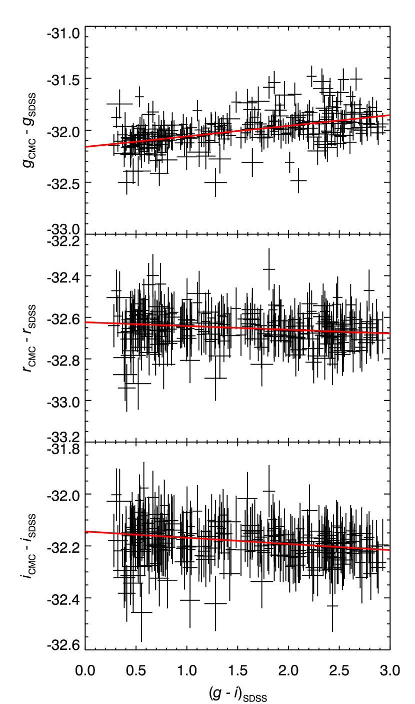
Figure 1.— Clay-Megacam color-term measurement. Data points are the photometry of point sources that have been matched between the Clay-Megacam and IMACS catalogs, the latter of which has already been transformed to the SDSS system. The best-fit lines, whose slopes are equal to the color-term coefficients, are also shown.

The systematic uncertainty of the color calibration is estimated at $0.01\,\mathrm{mag}$ to $0.03\,\mathrm{mag}$ in $g-r$ and $r-i$, likely dominated by the non-uniformity of Galactic extinction, flat-fielding, and details of the photometry (see High et al., 2009). Magnitude calibrations are uncertain at $\sim 0.05\,\mathrm{mag}$ in all bands, dominated by the overall accuracy of the 2MASS point-source catalog. These levels of uncertainty are sufficient for our purposes.

Table 2 lists the basic imaging information for the five clusters. Depths are estimated from the median magnitude of sources whose signal-to-noise ratio is 5. Seeing is estimated in the WL band, $r^{\prime}$.

Table 2Imaging data

Cluster Name	Magnitude of $5\sigma$ Point Source			$r$ Seeing
	$g$	$r$	$i$
SPT-CL J0516-5430	27.1	26.7	26.0	$0\farcs 67$
SPT-CL J2022-6323	26.3	26.2	25.3	$0\farcs 88$
SPT-CL J2030-5638	26.4	26.2	25.4	$0\farcs 80$
SPT-CL J2032-5627	25.9	25.8	24.4	$0\farcs 82$
SPT-CL J2135-5726	26.6	26.1	25.4	$0\farcs 89$

Note. — Basic properties of the imaging of the five clusters.

Column 1: R12 cluster designation.

Columns 2–4: the median magnitude of sources whose signal-to-noise ratio is 5.

Column 5: the median of the stellar FWHM across the entire coadded image.

We test the effect of photometric zeropoint errors on the final WL-SZ mass ratios. Systematic errors in photometry enter into the mass analysis through the estimation of the critical surface density for each cluster (Section 4.2). We estimate this quantity using publicly available photometric redshift catalogs of external fields, to which we apply the same photometric cuts as are applied to the Megacam catalogs. If there is an offset in the Megacam $i^{\prime}$-band zeropoint relative to that of the standard catalog, then we effectively probe a population that is different than that from which we infer the source redshift distribution. We test the effect of photometric error, $\delta_{i}$, by cutting the standard photo-$z$ catalogs at $i_{\mathrm{CFHT}}>24-\delta_{i}$ and repeating the full analysis. The level of photometric accuracy estimated here (5%) causes changes in the WL-SZ mass ratios at the sub-percent level, which is significantly subdominant to the statistical uncertainty and the largest systematic uncertainties.

4. Creating Shear Catalogs

In this section, we summarize the standard theoretical framework on which WL mass measurements rest, including the two primary quantities that must be estimated from data: the critical surface density and the reduced shear.

4.1. Tangential Shear

Weak gravitational lensing of extended sources by spherically symmetric mass overdensities induces a mean shear in a direction oriented tangentially to the center of mass. Tangential shear, $\gamma_{+}$, is calculated from the Cartesian components of shear, $(\gamma_{1},\gamma_{2})$, as

$$\gamma_{+}=-\gamma_{1}\cos(2\phi)-\gamma_{2}\sin(2\phi)$$ (4)

(see for example Mellier, 1999, Section 2, for an overview of WL shear). Indices $i\in\{1,2\}$ correspond to horizontal and vertical image coordinates. Here, $\gamma_{1}$ is the component along the horizontal axis (position angle $\phi=0^{\circ}$) and $\gamma_{2}$ is the shear at position angle $\phi=45^{\circ}$. Cross shear is calculated as

$$\gamma_{\times}=-\gamma_{1}\sin(2\phi)+\gamma_{2}\cos(2\phi);$$ (5)

this is the shear component oriented at $45^{\circ}$ with respect to $\gamma_{+}$. The azimuthally averaged cross shear $\langle\gamma_{\times}\rangle$ as a function of radius provides a diagnostic for residual systematics, because no astrophysical effects, including lensing, produce such a signal. As a consequence, a non-zero $\langle\gamma_{\times}\rangle$ indicates the presence of some types of residual systematic error, though we note that this is not an exhaustive test.

The mean tangential shear as a function of radial distance in the plane of the sky at the cluster redshift, $R$, depends on the projected surface density, $\Sigma(R)$, as

$$\langle\gamma_{+}\rangle(R)=\frac{\langle{\Sigma}\rangle({<R})-\Sigma(R)}{\Sigma_{\mathrm{crit}}}$$ (6)

(Miralda-Escude, 1995). This depends on the critical surface density,

$$\Sigma_{\mathrm{crit}}=\frac{c^{2}}{4\pi G}\frac{1}{D_{\mathrm{l}}\beta},$$ (7)

where $c$ is the speed of light, $G$ is the gravitational constant, and $\beta\equiv D_{ls}/D_{s}$ is the lensing efficiency. Quantities $D$ are angular-diameter distances, and $l$ indicates the lens (the cluster) while $s$ indicates sources.

The observable quantity is not the shear but the reduced shear, $g$, which relates to the shear as

$$\gamma=(1-\kappa)g$$ (8)

via the convergence, $\kappa=\Sigma/\Sigma_{\mathrm{crit}}$. Estimating true shear therefore requires estimating convergence, which we perform in radial bins, as discussed in Section 5.1.

The two key quantities in measuring mass from WL data are thus the critical surface density and the reduced shear. We describe these two steps in the following sections.

4.2. Cluster-galaxy Decontamination and Critical Surface Density Estimation

Calculating WL masses requires estimating the critical surface density (Equation (7)), which is a geometric quantity containing ratios of angular diameter distances between the observer, the lens, and sources. This requires redshift information for the lens and sources. Three bands are not sufficient for estimating source redshifts in the Clay-Megacam data themselves, so we rely on photometric redshift catalogs of other, non-overlapping surveys that have integrated to equal or greater depths, under the assumption that the mean underlying galaxy population is the same everywhere in the sky. The Canada-France-Hawaii Telescope Legacy Survey (CFHTLS) Deep field catalogs are sufficient for this purpose (Coupon et al., 2009). For the $\Sigma_{\mathrm{crit}}$ estimate from the photo-$z$ catalog to accurately reflect the population in the Clay-Megacam images on average, cluster galaxies must be removed from the Clay-Megacam catalogs.

We remove cluster galaxies from the shear catalogs using the same CFHTLS catalogs as a guide. We first plot the density of galaxies at $19<i_{\mathrm{CFHT}}<25$ in the CFHTLS-Deep catalogs in $(g-r,r-i)$ color–color space. Galaxies with photometric redshifts of $|z_{\mathrm{phot}}-z_{l}|<0.05$, i.e., near the cluster redshift, are considered contaminants or “non-sources”, and all other galaxies are considered “sources”. The densities of these two populations are shown in Figure 2. We then define a simple polygon that encloses the majority of the non-source galaxies.

Because the clusters are at different redshifts, the location and shape of this polygon is a function of $z_{l}$ in general. Rather than defining five different polygons, we only define two: one that excises cluster galaxies for $0.28<z_{l}<0.35$ (two clusters), and one for $0.35<z_{l}<0.43$ (three clusters). Figure 3 shows the photometric redshift distribution after removing galaxies within the high-$z_{l}$ polygon. We test the contamination after cuts by using these polygons to remove galaxies from the CFHTLS-Deep catalogs, and measuring the fraction of galaxies with photometric redshifts satisfying $|z_{\mathrm{phot}}-z_{l}|<0.05$. Under this test, the fraction of contaminants is $<0.1\%$ for all cluster redshifts considered here.

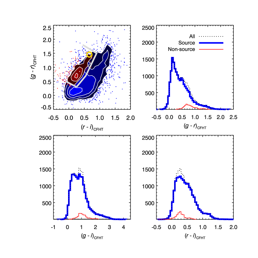
Figure 2.— Color–color distribution of $19<i_{\mathrm{CFHT}}<25$ galaxies in the CFHTLS-Deep photometric redshift catalog. Upper left: the blue region denotes the distribution of source galaxies ($|z_{\mathrm{phot}}-z_{\mathrm{l}}|>0.05$), and red denotes non-source galaxies ($|z_{\mathrm{phot}}-z_{\mathrm{l}}|<0.05$), both for an example cluster in the high redshift bin, SPT-CL J2022-6323 at $z_{l}=0.383$. Contours delineate isodensities in color–color bins of size $0.1\,\mathrm{mag}\times 0.1\,\mathrm{mag}$, and are logarithmically spaced by factors of $10^{0.5}$ starting at 10. The gray polygon delineates source/non-source regions. The yellow circle shows the typical color of a luminous red galaxy at the cluster redshift (Lopes, 2007). The remaining panels show one-dimensional histograms of projections of these colors. These panels illustrate that one-dimensional color cuts are a less efficient way of removing contaminant galaxies.

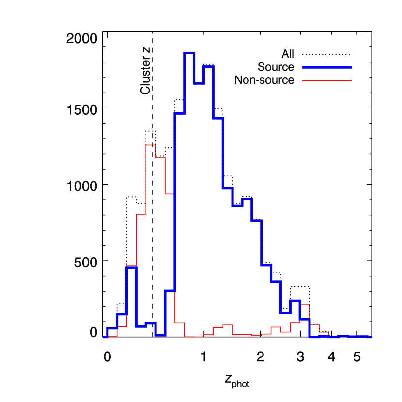
Figure 3.— CFHTLS Deep field 3 photo-$z$ distribution of $19<i_{\mathrm{CFHT}}<25$ galaxies after we have identified sources and non-sources using the color cuts illustrated in Figure 2. A redshift of $0.383$, corresponding to SPT-CL J2022-6323, is shown.

After transforming the Clay-Megacam catalogs to the CFHT-Megacam photometric system using color terms (Regnault et al., 2009), we apply the same magnitude and color cuts to the Clay-Megacam catalogs. The radial distribution of catalog galaxies before and after the color cuts is shown in Figure 4 for a representative cluster. This procedure removes most of the radially decreasing trend of galaxy densities such that the final galaxy surface density is uncorrelated with radius. This constitutes some empirical evidence that the procedure is removing cluster galaxies. Some residual surface density trend with radius may be expected due to WL magnification (e.g. Bartelmann & Schneider, 2001). We measure the slope of $\mathrm{d}\log{N}/\mathrm{d}m$ of selected sources to be $\sim 0.4$ in our data, so the effect would be small.

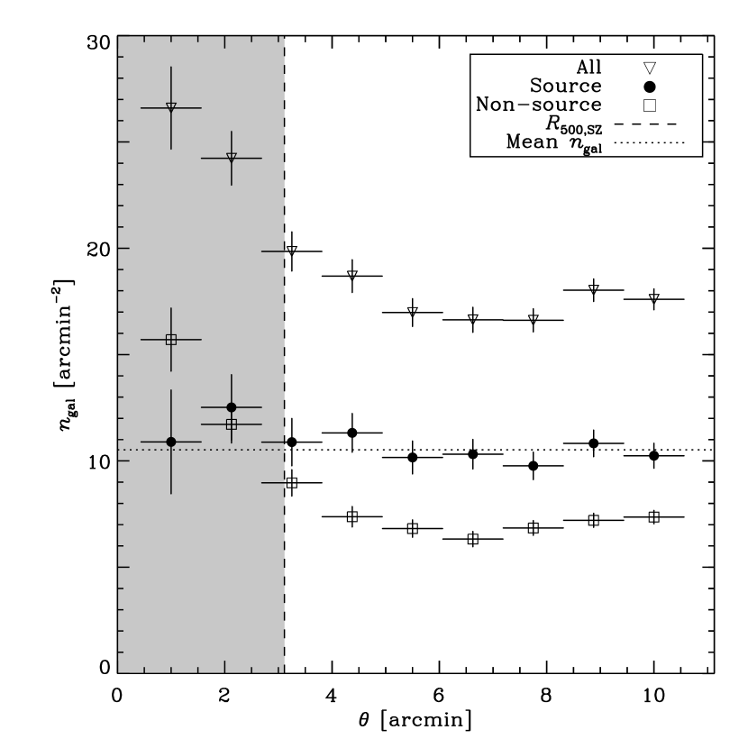
Figure 4.— Radial distribution of galaxies in the Clay-Megacam catalog of cluster SPT-CL J2022-6323, before and after making the color cuts described in Section 4.2. These data are representative of all clusters. The color cuts reduce the clustering signal such that the final catalog used in the weak lensing analysis is roughly flat. WL masses are computed outside the shaded region, from $\theta_{1}$ (vertical dashed line) to $\theta_{2}=12\arcmin$.

We estimate $\langle\beta\rangle$ and $\langle\beta^{2}\rangle$ from the photo-$z$ distribution in the CFHTLS-Deep catalogs after these selections are made (Figure 3). The $\beta$ distribution is expected to vary between fields, both in the CFHTLS Deep fields and the SPT cluster fields, due to finite galaxy counts and cosmic variance. We estimate the uncertainty this induces in the mean mass ratio results by repeating the entire analysis using each CFHTLS Deep field individually, and averaging the results. The uncertainties on resulting WL to SZ mass ratios are $<2\%$, a level that is subdominant to the overall statistical uncertainties and other systematics. We adopt the mean values of $\langle\beta\rangle$ and $\langle\beta^{2}\rangle$ over the four CFHTLS Deep fields in the baseline analysis. These are reported in Table 3.

Table 3Source galaxy properties.

Cluster Name	$z_{l}$	$\langle\beta\rangle$	$\langle\beta^{2}\rangle$	$n_{\mathrm{gal}}$
				(arcmin-2)
SPT-CL J0516-5430	0.294(1)	0.64	0.43	14.8
SPT-CL J2022-6323	0.383(1)	0.54	0.32	10.6
SPT-CL J2030-5638	0.40(4)	0.53	0.31	13.3
SPT-CL J2032-5627	0.284(1)	0.65	0.44	19.0
SPT-CL J2135-5726	0.427(1)	0.50	0.29	12.2

Note. — This table summarizes the basic properties of the sources used in the weak-lensing mass measurement after making the catalog selections described in Section 4.2.

Column 1: R12 cluster designation.

Column 2: cluster redshift. The number in parentheses is the uncertainty in the last digit.

Column 3: the mean of $\beta=D_{ls}/D_{s}$ after cuts.

Column 4: the variance of $\beta$ after cuts.

Column 5: the source number density after cuts.

We perform consistency checks on the WL mass analysis by modifying this photometric selection procedure in two ways. First, we test defining color–color polygons that remove the vast majority of objects at $z_{\mathrm{phot}}<z_{l}+0.1$, i.e., both near and in front of the cluster. This significantly widens the area covered by the polygon, and the effect is that a large number of galaxies that are in fact behind the cluster are eliminated as well. This roughly halves $n_{\mathrm{gal}}$ and does not change $\langle\beta\rangle$ estimates significantly. The WL-SZ ratios are consistent with unity and with the baseline result under this test.

Second, we test using limits of $i_{\mathrm{CFHT}}=24.5$ and $24$, which are brighter than our baseline limit of $i_{\mathrm{CFHT}}=25$. The effect is to probe a brighter mean population of galaxies in the catalogs, which causes $\langle\beta\rangle$ and $n_{\mathrm{gal}}$ to both take smaller values. This increases the statistical uncertainty of the WL masses, but restricts the catalogs to magnitude regimes in which the CFHTLS-Deep photometric redshift catalogs have been explicitly tested and verified (Coupon et al., 2009). The resulting WL-SZ aperture mass ratios in both cases are statistically consistent with the baseline result, and with unity.

4.3. Shear Measurement Method

The second key ingredient in estimating cluster masses in WL analyses is reduced shear. To estimate reduced shear in the $r^{\prime}$-band images we employ the method of Kaiser, Squires, & Broadhurst (1995, hereafter KSB) and Luppino & Kaiser (1997), with the modifications of Hoekstra et al. (1998). This method bases shear measurements on Gaussian-weighted second-order image moments,

$$I_{ij}=\int d^{2}\vec{x}x_{i}x_{j}W(\vec{x})f(\vec{x}),$$ (9)

where $W$ is the Gaussian function, $f$ is the object image, and the origin of the coordinate system has been iteratively determined from the first-order moment using the same weight. Variables $x_{i}$ ($i\in\{1,2\}$) indicate vertical and horizontal image coordinates. The polarization is a spin 2 pseudo-vector $e_{\alpha}$ ($\alpha\in\{1,2\}$), where

$$e_{1}=\frac{I_{11}-I_{22}}{I_{11}+I_{22}}\quad\mathrm{and}\quad e_{2}=\frac{2I_{12}}{I_{11}+I_{22}}.$$ (10)

The magnitude of the polarization is $e=(e_{1}^{2}+e_{2}^{2})^{1/2}$.

The resulting polarizations must be corrected for the effects of the anisotropic smearing by the PSF. To this end, we fit fourth order polynomials to the stellar $P^{\mathrm{sh}}_{ii}$ and $P^{\mathrm{sm}}_{ii}$ (the diagonal entries of the shear- and smear-polarizability tensors, see KSB) and remove outliers. To the surviving objects we fit a fourth order polynomial to both $e_{1}$ and $e_{2}$. We do this for a range of weight functions, which is necessary for computing the pre-seeing shear polarizability $P^{\gamma}$ (see Hoekstra et al., 1998). The rms of the residuals for each polarization component after the fourth order fit are $<0.005$ for all clusters. These are small compared to the magnitude of signals we are seeking, which are about $0.01$ to $0.1$. While residuals of this size can in principle lead to large shear bias for any given faint galaxy locally, we expect this effect to be zero on average in the radial bins because the spatial residual pattern is consistent with noise. A representative example PSF polarization plot is shown in Figure 5. This model is used to correct for PSF anisotropy using the procedure described in the original works (KSB; Hoekstra et al., 1998).

Figure 5.— PSF polarization plot of the coadded $r$-band image of SPT-CL J2022-6323, which is representative of the sample. Left: polarization magnitude and direction, as measured from the Gaussian-weighted image moments of point sources. Right: same as the left panel, after a fourth order polynomial in the two spatial dimensions is fit to each component of polarization. Residuals between the data and the model are $<0.005$ rms for all clusters.

The next step is to account for the seeing, which lowers the observed shear signal. This is done by rescaling the polarizations to their “true” values by $P^{\gamma}$ (Luppino & Kaiser, 1997; Hoekstra et al., 1998). The measurements of $P^{\gamma}$ for individual galaxies are too noisy, and instead we bin the measurements in galaxy size and use this to compute the value as a function of size. The reduced shear $g$ is then estimated as

$$g_{i}=e_{i}/P^{\gamma}.$$ (11)

This implementation of the KSB shear analysis pipeline is described in more detail in previous works (Hoekstra et al., 1998, 2000). It was subject to blind tests by the Shear Testing Program (Heymans et al., 2006; Massey et al., 2007), wherein it achieved accuracy at the $0.02\gamma$ level under low PSF anisotropies, such as Clay-Megacam exhibits. This level of bias induces mass errors that are subdominant to the statistical and systematic uncertainties.

5. Weak-lensing Mass Measurement

In this section we discuss how we estimate mass from the shear catalogs. We employ two types of WL mass estimators, both of which make use of the same, azimuthally averaged shear profiles. We test the accuracy of our algorithms using ray-traced $N$-body simulations, and we also describe the WL convergence field reconstruction procedure.

5.1. Shear Profiles and Corrections

We compute binned shear profiles using a weighted average in each radial bin. The weight for each galaxy is

$$w=\frac{1}{\sigma^{2}_{g}}=\frac{P^{\gamma\,2}}{\sigma_{\gamma}^{2}P^{\gamma\,2}+\langle\Delta e^{2}\rangle},$$ (12)

where $\sigma_{\gamma}$ is the scatter in shear due to the intrinsic ellipticity of the galaxies (set to 0.3; see for example Leauthaud et al., 2007) and $\langle\Delta e^{2}\rangle$ is the error estimate for the polarization (Hoekstra et al., 2000). The weighted mean for $i\in\{+,\times\}$ is then

$$\langle\gamma_{i}\rangle=\frac{\sum_{n}w_{n}\gamma_{i,n}}{\sum_{n}w_{n}},$$ (13)

and errors on the mean, $\sigma_{\langle\gamma_{i}\rangle}$, are computed via

$$\frac{1}{\sigma_{\langle\gamma_{i}\rangle}^{2}}=\sum_{n}w_{n}.$$ (14)

Two corrections are applied to the binned shear data. The first correction accounts for a known error in the binned shear data due to the averaging operation. Seitz & Schneider (1997) show that estimating the critical surface density of each cluster using the mean of the $\beta$ distribution in redshift catalogs induces an error in the observed reduced-shear, which can be corrected to first order using

$$\frac{\langle g_{\mathrm{obs}}\rangle}{\langle g_{\mathrm{true}}\rangle}=1+\left(\frac{\langle\beta^{2}\rangle}{\langle\beta\rangle^{2}}-1\right)\kappa.$$ (15)

We adopt the model for $\kappa$ described below to make this correction.

The second correction is to transform the reduced shear $g$ to shear $\gamma$ by estimating the $\kappa$ in each bin. We accomplish this by jointly fitting for the shear and the convergence profiles to those predicted by Navarro, Frenk, & White (1997, hereafter NFW) density profiles assuming Duffy et al. (2008, hereafter D08) concentration–mass–redshift scaling, wherein the SZ-derived mass is used as the input. The NFW family of density profiles take the form

$$\rho(r)=\frac{\delta_{c}\mbox{$\rho_{\mathrm{crit}}$}}{(rc/r_{200})(1+rc/r_{200})^{2}},$$ (16)

where $r$ is the three-dimensional radial distance, $r_{200}$ is the radius at which the mean NFW overdensity is 200 times $\rho_{\mathrm{crit}}$ at the cluster redshift, $c$ is concentration, and

$$\delta_{c}=\frac{200}{3}\frac{c^{2}}{\ln(1+c)-c/(1+c)}.$$ (17)

This fitting procedure results in estimates of the $\gamma$ profile under the assumption of D08 concentrations, and it also yields the convergence profile used to perform the redshift distribution correction in Equation 15 as well as total spherical masses in our main results.

Observed shear profiles, after all of these corrections are applied, are presented in the Appendix. The cross shear is consistent with zero, as expected for a signal that is not appreciably contaminated by systematics.

5.2. Aperture Masses

One of the advantages of the tangential shear is that it can be used to directly constrain the projected mass within an aperture. Aperture masses are integrals over the shear data multiplied by a filter (see Fahlman et al., 1994; Schneider, 1996). These aperture masses are parameter-free in the sense that the observable quantity gives cylindrical mass constraints without reference to analytic density profiles. If the filter is compensated, they are also insensitive to the mass-sheet degeneracy. The classical $\zeta$-statistic for circular apertures, which uses a particular choice of filter, is

$$\begin{split}\zeta(\theta_{1})&=\langle\kappa\rangle_{<\theta_{1}}-\langle\kappa\rangle_{\theta_{1}<\theta<\theta_{2}}\\ &=\frac{2}{1-\theta_{1}^{2}/\theta_{2}^{2}}\int_{\theta_{1}}^{\theta_{2}}\mathrm{d}\theta\,\frac{\langle\gamma_{+}\rangle(\theta)}{\theta}\end{split}$$ (18)

(Fahlman et al., 1994; Kaiser, 1995). The aperture mass is then

$$M_{\mathrm{ap}}(\theta_{1})=\pi(\theta_{1}D_{l})^{2}\Sigma_{\mathrm{crit}}\zeta(\theta_{1}).$$ (19)

The square of the measurement uncertainty of the aperture mass statistic takes an analytic form,

$$\sigma^{2}_{\mathrm{stat}}(\theta_{1})=\left(\frac{2}{1-\theta_{1}^{2}/\theta_{2}^{2}}\right)^{2}\int_{\theta_{1}}^{\theta_{2}}\mathrm{d}\theta\,\frac{\sigma_{\langle\gamma_{+}\rangle}^{2}}{\theta^{2}},$$ (20)

where $\sigma_{\langle\gamma_{+}\rangle}$ is given in Equation (14). In addition to the measurement uncertainty, LSS along the line of sight contributes a random uncertainty to the WL aperture masses, which we add to the formal statistical WL mass uncertainties in quadrature using the prescription of Hoekstra et al. (2011). LSS uncertainties are 15% to 20% for these clusters.

We fix $\theta_{2}$ to $12\arcmin$ for all analyses, which is roughly the maximum radius of the Megacam imaging. We set $\theta_{1}$ to $R_{\mathrm{500,SZ}}/D_{l}$.

Aperture masses provide lower limits on total cylindrical masses within $\theta_{1}$. In the limit of $\theta_{2}\to\infty$, the aperture mass converges to true integrated cylindrical mass within $\theta_{1}$, but real data extend to finite radius, so $\theta_{2}$ must be finite. Direct comparisons of the observed aperture mass to other spherical or cylindrical mass-observables therefore requires care.

5.3. Spherical- to Aperture-mass Transformations

Some extra computation makes direct comparisons between aperture masses and spherical masses possible. This is accomplished by assuming an analytic three-dimensional profile consistent with a given spherical mass estimate, projecting it to two dimensions, calculating the shear assuming some $\Sigma_{\mathrm{crit}}$, and then computing the aperture mass statistic given this predicted shear.

To illustrate this procedure concretely, say we are given some spherical mass estimate, $M_{\Delta,\mathrm{obs}}$, derived from another observable such as the SZ effect. We wish to compare this to the WL aperture mass at the same radius, $M_{\mathrm{ap,WL}}(R_{\Delta,\mathrm{obs}})$, where $R_{\Delta,\mathrm{obs}}=[3M_{\Delta,\mathrm{obs}}/(\Delta 4\pi\rho_{\mathrm{crit}}(z_{l}))]^{1/3}$. We first assume a three-dimensional NFW profile, with total spherical mass within $R_{\Delta,\mathrm{obs}}$ equal to $M_{\Delta,\mathrm{obs}}$, and concentration $c$ taken from the mean of clusters of these masses and redshifts according to the D08 $c$–$M$–$z$ scaling relation. The corresponding two-dimensional projection of this profile and predicted shear take an analytic form (Wright & Brainerd, 2000). We use the same $\Sigma_{\mathrm{crit}}$ as used in the WL analysis. Then, from this shear we compute $\zeta$, again using the same filter as used on the WL data. Specifically, the outer radius, $\theta_{2}=12\arcmin$, has been set by the size of the Megacam imaging footprint, and the inner radius is $\theta_{1}=R_{\Delta,\mathrm{obs}}/D_{l}$. The result, $M_{\mathrm{ap,obs}}(R_{\Delta,\mathrm{obs}})$, is the aperture-equivalent mass of $M_{\Delta,\mathrm{obs}}$, which was determined by some other method or observable. It is the direct analog of the WL aperture mass measured at the same radius, $M_{\mathrm{ap,WL}}(R_{\Delta,\mathrm{obs}})$, such that the ratio of the WL to this aperture-equivalent quantity is unity in the absence of other systematic errors. We perform this transformation on SZ mass estimates to test for statistical consistency with the WL aperture masses.

We propagate spherical mass uncertainties to aperture mass equivalent by computing the aperture mass of $M_{\Delta,\mathrm{obs}}\pm\sigma_{M}$ numerically using the same procedure. As illustration, aperture mass uncertainties are $\sim(0.54,0.67,0.81)$ times the values of their spherical NFW counterparts for $c=(1,3,10)$ at these clusters’ typical $R_{500}$ radii.

5.4. Calibration Tests with Mock Catalogs

A number of recent works have shown using $N$-body simulations that WL derived mass estimates are biased at roughly the $-5\%$ to $-10\%$ level (Becker & Kravtsov, 2011; Bahé et al., 2012; Rasia et al., 2012). We perform similar calibration tests of the WL mass statistics presented in our work using mock shear catalogs of $220\deg^{2}$ of sky. The catalogs are drawn from an $N$-body dark matter simulation of a standard $\Lambda$CDM universe. The dark matter halos are populated with galaxies using ADDGALS such that they reproduce known luminosity, color, and clustering relations (Wechsler, 2004, R. H. Wechsler et al., in preparation). Shears are assigned to each galaxy by raytracing through the $N$-body simulation.

We compute the masses of $280$ $N$-body halos at redshifts $0.25<z<0.45$ with masses $M_{200}\geq 10^{14}h_{70}^{-1}\mbox{$M_{\odot}$}$. To reflect the choices we have made in analyzing the Clay-Megacam data, we only use shear profiles between $R_{500}$ and $12\arcmin$, where $R_{500}$ is extrapolated using the D08 concentration–mass–redshift scaling relation with $M_{200}$ determined from the $N$-body halo finder as the input. In order to minimize statistical uncertainty in these tests, we use perfect knowledge of the shear field at the galaxy locations (i.e., we do not include intrinsic shape noise) as well as perfect source redshifts, and we select source galaxies as those at $|z-z_{\mathrm{l}}|>0.05$. The resulting bias between measured masses and appropriately transformed $N$-body masses, averaged over the sample, ranges from $-6\%$ to $-13\%$, consistent in magnitude and sign with the previous works. These tests carry a statistical uncertainty of about $2\%$. The precise bias values are reported in Section 6.2. We do not apply these bias corrections to any mass estimates presented in this work.

5.5. Convergence Field Reconstruction

We reconstruct the convergence field in two dimensions using the method of Kaiser & Squires (1993). The purpose is to test the impact of using the peak of the reconstructed $\kappa$ field as the cluster center when computing shear profiles. The convergence is estimated up to a constant as a sum over galaxies $n$,

$$\kappa(\vec{x}_{0})=-\frac{1}{n_{\mathrm{gal}}\pi}\sum_{n}\chi_{\alpha}(\vec{x}_{n}-\vec{x}_{0})2e_{\alpha}/P^{\gamma},$$ (21)

where $n_{\mathrm{gal}}$ is the mean surface density of source galaxies and $\chi_{\alpha}=\{x^{2}-y^{2},2xy\}/\theta^{4}$ and $\theta=(x^{2}+y^{2})^{1/2}$. The constant is set such that the mean convergence across the full field is zero. The wide field-of-view of the observations allows us to avoid artifacts from this method which have caused problems in the past.

We pixelate the convergence maps at $0\farcm 4\,\mathrm{pixel}^{-1}$. The errors per pixel are independent, and are computed as $\sigma_{\mathrm{pix}}\approx\sigma_{\kappa}/\sqrt{n_{\mathrm{gal}}0\farcm 4^{2}}$, where $\sigma_{\kappa}\sim\sigma_{\gamma}\sim 0.3$ and $n_{\mathrm{gal}}$ is measured from the data and assigned units of $\mathrm{arcmin}^{-2}$. We then smooth the map with a Gaussian of size $\sigma_{\mathrm{smooth}}=3\arcmin$. The peak in the smoothed convergence field, $\max(\kappa)$, is identified as the maximum value across the entire smoothed map. The signal-to-noise ratio in the smoothed peak value is $\mathrm{S}/\mathrm{N}=\max(\kappa)/(\sigma_{\mathrm{pix}}/\sqrt{2\pi\sigma_{\mathrm{smooth}}/0\farcm 4})$. The uncertainty on the peak position is then $\mathrm{FWHM}_{\mathrm{smooth}}/(S/N)$, where $\mathrm{FWHM}_{\mathrm{smooth}}=\sqrt{8\ln{2}}\,\sigma_{\mathrm{smooth}}$. This is equal to $\sim 45\arcsec$ for all five clusters. Using the convergence field peaks as the cluster centers gives a mean ratio of WL-SZ masses that is consistent with unity and with the baseline result to within the statistical uncertainty.

6. Results

We report WL-derived masses, then test the overall accuracy of the SZ mass determination of R12 by measuring the mean ratio of equivalent WL and SZ mass estimators. In the baseline analysis we

• select source galaxies at $19<i_{\mathrm{CFHT}}<25$ with colors exterior to the polygon shown in Section 4.2,

• use concentrations of D08, and

• use SZ centroid as the cluster centers.

We then alter various steps in the analysis in order to test the robustness of the result, as well as to estimate the magnitude of various potential sources of error. Shear profiles and aperture mass profiles are presented in the Appendix, in addition to optical, SZ, and convergence maps.

6.1. Masses and Mass Ratios

In this section we use three different methods for estimating mass from these data. In all cases, we only use shear data at $R_{500,\mathrm{SZ}}/D_{l}<\theta<12\arcmin$.

In the first method, we measure aperture masses with $\theta_{1}=R_{500,\mathrm{SZ}}/D_{l}$ and $\theta_{2}=12\arcmin$. Following the procedure outlined in Section 5.3, we derive the equivalent estimator from the SZ masses by assigning an NFW profile consistent with $M_{500,\mathrm{SZ}}$, computing the predicted shear for such a profile, and then calculating the aperture mass from the predicted profile over the same radii. These masses are inherently projected, two-dimensional quantities. We plot the results in the top panel of Figure 6.

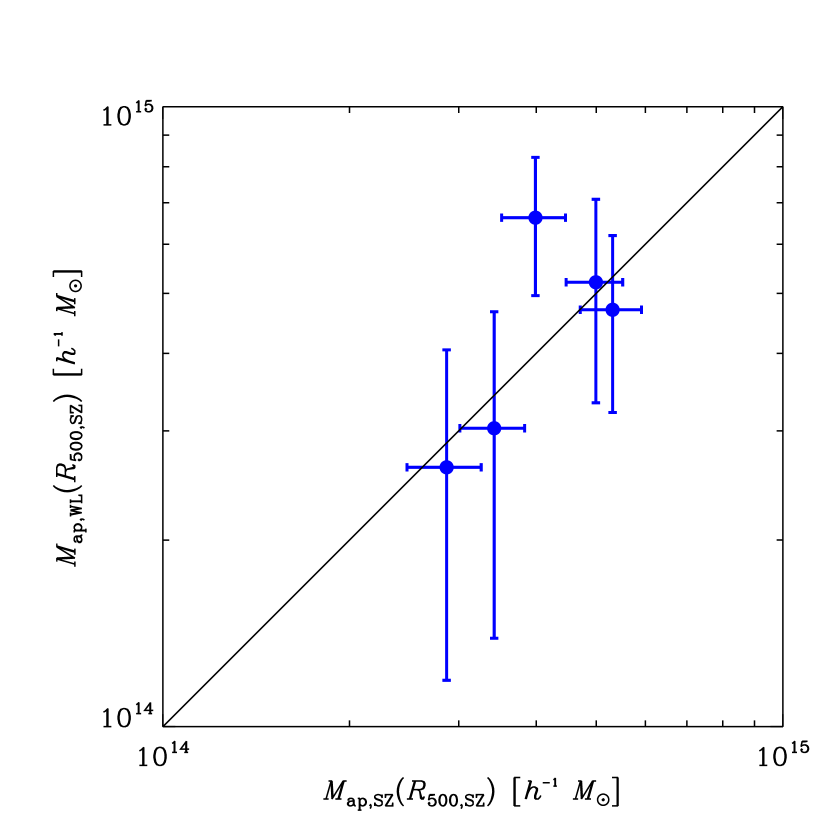
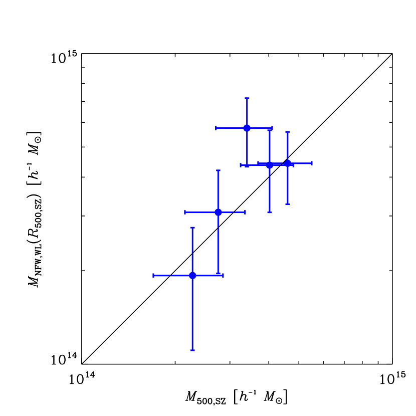
Figure 6.— Top: weak-lensing aperture masses vs. inferred aperture masses from Sunyaev–Zel’dovich effect data. The one-to-one line is also shown. Bottom: spherical WL masses vs spherical SZ masses. The WL masses are determined by fitting NFW profiles to weak lensing shear data at $R_{500,\mathrm{SZ}}/D_{l}<\theta<12\arcmin$ and evaluating the resulting NFW mass profile at $R_{500,\mathrm{SZ}}$.

In the second method, we estimate the spherical mass by fitting NFW profiles to binned shear data at $R_{500,\mathrm{SZ}}/D_{l}<\theta<12\arcmin$ and computing the total mass of the best fit profile at $R_{500,\mathrm{SZ}}$. We label this $M_{\mathrm{NFW,WL}}(R_{500,\mathrm{SZ}})$. The results are to be compared to $M_{500,\mathrm{SZ}}$ directly. Because of the use of a radius from an external source, the radius at which the mass is quoted is not the radius where $\Delta=500$ (the overdensity factor with respect to the cosmological critical density) in the best-fit NFW model. These masses are plotted in the bottom panel of Figure 6.

And in the third method, we use the same best-fit profiles above to estimate the spherical mass within the radius where $\Delta=500$ as determined from the best-fit model itself, i.e., $M_{500,\mathrm{WL}}$. This is also to be compared to $M_{500,\mathrm{SZ}}$ directly. These masses are plotted in Figure 7.

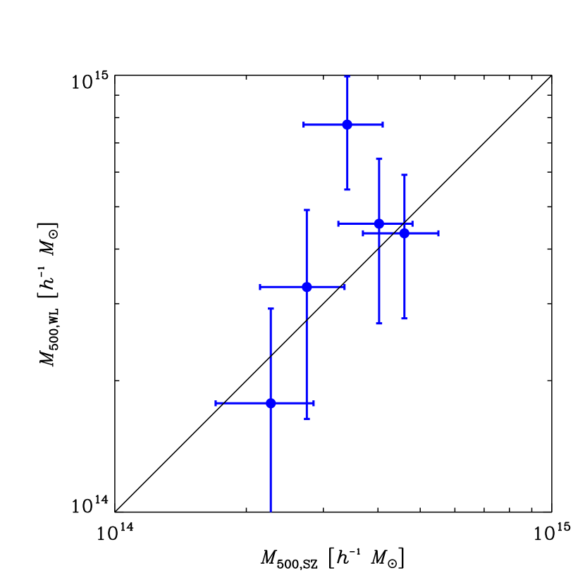
Figure 7.— Spherical WL masses vs spherical SZ masses. The WL masses are determined by fitting NFW profiles to weak lensing shear data at $R_{500,\mathrm{SZ}}/D_{l}<\theta<12\arcmin$ and evaluating the resulting NFW mass profile at $R_{500,\mathrm{WL}}$ as determined from the best-fit profile itself.

The expectation of the ratio of WL to SZ masses is unity for all of these methods in the absence of systematic errors from, for example, the concentration and cluster centering assumptions. We note that we use a concentration–mass–redshift scaling relation in all ratio tests: for the aperture mass comparison, it is only used to transform the SZ-derived mass to an aperture mass equivalent, whereas for both spherical mass comparisons it is only used in the WL shear profile fit.

The mass results and derived quantities are reported in Table 4.

Table 4Cluster mass results

Cluster Name	$R_{500,\mathrm{SZ}}$	$M_{\mathrm{ap,WL}}(R_{500,\mathrm{SZ}})$	$M_{\mathrm{ap,SZ}}(R_{500,\mathrm{SZ}})$	$M_{\mathrm{NFW,WL}}(R_{500,\mathrm{SZ}})$	$M_{500,\mathrm{WL}}$	$M_{500,\mathrm{SZ}}$
	($h^{-1}\mathrm{Mpc}$)	($10^{14}h^{-1}\mbox{$M_{\odot}$}$)	($10^{14}h^{-1}\mbox{$M_{\odot}$}$)	($10^{14}h^{-1}\mbox{$M_{\odot}$}$)	($10^{14}h^{-1}\mbox{$M_{\odot}$}$)	($10^{14}h^{-1}\mbox{$M_{\odot}$}$)
SPT-CL J0516-5430	0.84	$4.70\pm 1.49$	$5.31\pm 0.60$	$4.43\pm 1.16$	$4.35\pm 1.57$	$4.60\pm 0.90$
SPT-CL J2022-6323	0.69	$3.03\pm 1.64$	$3.42\pm 0.41$	$3.08\pm 1.12$	$3.27\pm 1.64$	$2.75\pm 0.60$
SPT-CL J2030-5638	0.64	$2.62\pm 1.43$	$2.87\pm 0.39$	$1.93\pm 0.82$	$1.77\pm 1.15$	$2.28\pm 0.57$
SPT-CL J2032-5627	0.77	$6.62\pm 1.66$	$3.99\pm 0.47$	$5.75\pm 1.43$	$7.71\pm 2.23$	$3.40\pm 0.70$
SPT-CL J2135-5726	0.77	$5.21\pm 1.88$	$4.99\pm 0.52$	$4.37\pm 1.29$	$4.57\pm 1.87$	$4.03\pm 0.78$

Note. — Results from the WL measurements, as well SZ data and derived quantities. We have divided two dimensional aperture masses from spherical masses.

Column 1: R12 cluster designation.

Column 2: cluster radius determined from the SPT SZ mass estimate in Column 7.

Column 3: WL aperture mass at $R_{500,\mathrm{SZ}}$.

Column 4: SZ aperture mass at $R_{500,\mathrm{SZ}}$.

Column 5: WL mass at $R_{500,\mathrm{SZ}}$ from NFW profile fitted to shear data at $R_{500,\mathrm{SZ}}/D_{l}<\theta<12\arcmin$.

Column 6: WL mass at $R_{500,\mathrm{WL}}$ from NFW profile fitted to shear data at $R_{500,\mathrm{SZ}}/D_{l}<\theta<12\arcmin$.

Column 7: SZ mass estimate from R12.

The mean ratios of the three WL to SZ mass statistics are summarized in Table 5. In all cases we report weighted mean values, where, for each cluster $n$, weights $1/\sigma_{n}^{2}$ are a combination of the WL aperture mass statistical uncertainty (including the estimated LSS contribution, which is between 15% and 20% for these clusters) and the total SZ mass uncertainties from R12 propagated to the derived quantity when necessary. The uncertainty on the mean is computed via $1/\sigma^{2}=\sum_{n}1/\sigma_{n}^{2}$.

Table 5Mass ratio results and consistency tests

Procedure	Aperture Masses		Spherical Masses at $R_{500,\mathrm{SZ}}$		Spherical Masses at $R_{500,\mathrm{WL}}$
	Mean Ratio	Total Scatter	Mean Ratio	Total Scatter	Mean Ratio	Total Scatter
		(%)		[%]		(%)
Baseline results	$1.04\pm 0.18$	33	$1.07\pm 0.18$	33	$1.10\pm 0.24$	58
$i_{\mathrm{CFHT}}<24.5$	$1.05\pm 0.20$	37	$1.05\pm 0.19$	37	$1.08\pm 0.25$	65
$i_{\mathrm{CFHT}}<24.0$	$1.07\pm 0.23$	34	$1.07\pm 0.21$	35	$1.12\pm 0.29$	60
Conservative color cuts	$1.07\pm 0.19$	35	$1.12\pm 0.18$	35	$1.16\pm 0.23$	58

Note. — WL-SZ mass ratio results. The baseline analysis employs a magnitude limit of $i_{\mathrm{CFHT}}=25$ and color cuts described in Section 4.2.

Column 1: procedure used to compute mean ratio.

Column 2: weighted mean of the ratio of WL to SZ aperture masses, $\langle M_{\mathrm{ap,WL}}(R_{500,\mathrm{SZ}})/M_{\mathrm{ap,SZ}}(R_{500,\mathrm{SZ}})\rangle$.

Column 3: the unweighted standard deviation of the WL to SZ aperture mass ratio.

Column 4: weighted mean of the ratio of WL spherical mass (evaluated at $R_{500,\mathrm{SZ}}$) to SZ spherical mass, $\langle M_{NFW,\mathrm{WL}}(R_{500,\mathrm{SZ}})/M_{500,\mathrm{SZ}}\rangle$.

Column 5: the unweighted standard deviation of the Column 4 ratio statistic.

Column 6: weighted mean of the ratio of WL spherical mass (evaluated at $R_{500,\mathrm{WL}}$) to SZ spherical mass, $\langle M_{500,\mathrm{WL}}/M_{500,\mathrm{SZ}}\rangle$.

Column 7: the unweighted standard deviation of the Column 6 ratio statistic.

We note that this method does not take into account any correlated uncertainty between clusters. The SZ mass estimates from R12 have been marginalized over cosmological and scaling relation parameters, and this results in a $\sim 10\%$ systematic uncertainty that is highly correlated between clusters. We have checked for the effect of these correlations. Briefly, we adopt a Gaussian likelihood for both the SZ and WL mass statistics and introduce nuisance parameters representing the true mass of each cluster. We introduce an additional free parameter representing an overall scaling of the SZ mass estimates. We then explore the resulting likelihood surface using an MCMC. If we use a diagonal covariance matrix with the uncertainties given in Table 4, we recover the nominal mean ratios of WL to SZ mass statistics of Table 5 at the maximum likelihood points in the chains. If we use the covariance matrix for the five clusters as estimated from the R12 cosmological chains, we find that the increase in the uncertainty on the mean ratios is small ($\sim 10\%$ of the baseline ratio uncertainty values) when compared to when we set these correlations to zero. As discussed in Section 6.2, WL systematic uncertainties are estimated to be significantly smaller than the statistical components, so we only use a diagonal WL covariance matrix. Thus, we ignore the correlated component to the SZ and WL cluster mass estimate uncertainties for the remainder of this work.

The total scatter reported in Table 5 is the unweighted standard deviation of the respective ratio data. We do not estimate intrinsic scatter because this requires an estimate of the level of correlation in intrinsic scatter between the WL and SZ mass-observables. Estimating these quantities is beyond the scope of this work (see Section 7.1 for further discussion).

We have performed additional consistency tests by using brighter $i_{\mathrm{CFHT}}$ magnitude limits, and by adopting more conservative color cuts. The brighter magnitude limits are meant to probe the CFHTLS-Deep catalogs at magnitudes where the photo-$z$ accuracy has been explicitly verified and stated (Coupon et al., 2009). Results of these tests are also reported in Table 5. For all tests we have performed, mean ratios are statistically consistent with unity and with the baseline result to within $1\sigma$.

6.2. Systematic Error Analysis

We have explored various potential sources of systematic error, as discussed throughout the text, and we report the effects on the mean WL-SZ mass ratios in Table 6 for the dominant or most interesting cases. Changes in mean ratios are quoted relative to the baseline results of the aperture mass and spherical mass comparisons (Table 5).

Table 6Possible sources of systematic error.

Perturbation	Change in Mean Ratio
	Aperture Masses	Spherical Masses at $R_{500,\mathrm{SZ}}$	Spherical Masses at $R_{500,\mathrm{WL}}$
Concentration assumption
Duffy et al. (2008) (baseline)	$+0.00$	$+0.00$	$+0.00$
Macciò et al. (2008)	$+0.03$	$+0.04$	$+0.06$
Neto et al. (2007)	$+0.02$	$+0.03$	$+0.04$
Prada et al. (2011) 50th percentile	$+0.04$	$+0.06$	$+0.08$
Prada et al. (2011) 90th percentile	$+0.06$	$+0.09$	$+0.11$
Cluster center assumption
Use BCG centers	$+0.00$	$-0.01$	$-0.02$
Use $\kappa$ map centers	$-0.14$	$-0.12$	$-0.17$
Other
Calibration to $N$-body simulation	$+0.06$	$+0.09$	$+0.13$

Note. — Exploration of possible sources of uncertainty in the WL-SZ mass ratios with respect to the baseline results shown in Table 5.

Column 1: brief description of the perturbation performed.

Column 2: change in weighted mean, $\langle M_{\mathrm{ap,WL}}(R_{500,\mathrm{SZ}})/M_{\mathrm{ap,SZ}}(R_{500,\mathrm{SZ}})\rangle$.

Column 3: change in weighted mean, $\langle M_{\mathrm{NFW,WL}}(R_{500,\mathrm{SZ}})/M_{500,\mathrm{SZ}}\rangle$.

Column 4: change in weighted mean, $\langle M_{500,\mathrm{WL}}/M_{500,\mathrm{SZ}}\rangle$.

Our first tests are to measure the effect that the assumed concentration scaling relation has on the mean ratios. Our baseline analysis uses that of D08, which gives $3.0\leq c\leq 3.2$ for these five clusters. The work of Macciò et al. (2008) give $4.2\leq c\leq 4.5$ and Neto et al. (2007) give $3.8\leq c\leq 4.1$. Prada et al. (2011) find concentration values higher than these other works, with 50th percentile values of $c\approx 5.0$ and 90th percentile values of $c\approx 7.1$. The latter represents the most extreme concentrations we might expect for this sample, while the D08 gives the lowest expected values. This range of concentrations change the aperture mass ratios by 2% to 6%. Spherical mass ratios using NFW fits to WL data evaluated at $R_{\mathrm{500,SZ}}$ change by 3% to 9%, and those evaluated at $R_{\mathrm{500,WL}}$ change by 4% to 11%. This level of uncertainty is less than our statistical uncertainty on the mass ratio for the five clusters, but it is the dominant source of systematic uncertainty in this work.

While we use the SZ positions as the cluster centers in the baseline analyses, we also test using two other definitions of the cluster center: (1) the BCG and (2) the peak in the WL-reconstructed $\kappa$ field. We use the BCGs selected of Song et al. (2012), which are typically $\lesssim 30\arcsec$ from the SZ centroid, with the exception of SPT-CL J2032-5627, which is nearly $2\arcmin$ away. Mean ratio results using the BCG as the cluster center are in near perfect agreement with those using the SZ positions. However, adoption of the $\kappa$ peak location as the cluster center reduces the mean ratios of aperture masses and spherical masses by significantly greater amounts. The $\kappa$ peak locations have statistical uncertainties of $\sim 30\arcsec$ to $60\arcsec$, which are the largest uncertainties of the three center choices we have considered. While the mean ratios using $\kappa$ peak locations are statistically consistent with unity and with the baseline results, this represents the largest deviation from the baseline. This is probably because of noise in centering due to the large statistical uncertainties in determining convergence field peak locations; indeed, the universal reduction in the ratio values using these centers provides some evidence that the convergence peaks are poorer estimators of cluster centers than the SZ and BCG positions given the data, as centering errors suppress shear profiles, particularly in the inner regions (George et al., 2012).

Tests using $N$-body simulations (Section 5.4) result in the calibration bias levels reported in Table 6. The statistical uncertainties of these calibration bias estimates are each $2\%$. We have not applied these bias corrections to any individual mass estimates nor to any mean mass ratio statistics presented in this work. We note that such bias corrections increase tension with the mean mass ratio expectation of unity by up to $1\sigma$ at most.

The effects of other known sources of systematic uncertainty are smaller than those of concentration. The shear measurement method is estimated to be accurate to $0.02\gamma$ in shear (Section 4), which translates to $\leq 2\%$ in the mean aperture mass ratio and $\leq 3\%$ in mean spherical mass ratios.

The source redshift distribution inferred from the four different CFHTLS Deep fields (Section 4.2) is expected to vary due to finite galaxy counts and cosmic variance. The source redshift distribution in the SPT cluster fields we have observed is also expected to vary across fields in the same way. We estimate the uncertainty this induces in the mean ratio results by repeating the entire analysis using each CFHTLS Deep field individually and averaging the results. Under the assumption of randomness, the mean aperture mass ratio carries an uncertainty from finite galaxy counts and cosmic variance of $\pm 1.1\%$, while the mean spherical mass ratios are affected at $\pm 1.0\%$ (using $R_{\mathrm{500,SZ}}$) and $\pm 1.6\%$ (using $R_{\mathrm{500,WL}}$). This uncertainty can in principle be reduced further by using standard photo-$z$ catalogs of additional, disparate fields, or by measuring photo-$z$’s directly in the SPT cluster fields, but this is not necessary given the data, as it is significantly subdominant to other uncertainties.

Bias and uncertainty from assumed cosmological parameters are also subdominant. We have assumed cosmological parameter values that are slightly different from the results of R12 (combining the 100 high purity SPT detected clusters with the CMB+BAO+$H_{0}$+SNe data). To estimate the bias and scatter this induces, we have tested marginalizing the WL to SZ mass ratios over the R12 $\Lambda$CDM chains that combine CMB+BAO+$H_{0}$+SNe+SPT_CL data. The results are that both the bias and statistical uncertainty due to cosmology are sub-percent in the mass ratio statistics, and are therefore significantly below those expected from other sources of potential error.

In summary, no potential sources of systematic error that we have explored contributes at or above the level of statistical accuracy for this sample of clusters, suggesting they are all subdominant. Uncertainty in the assumed NFW profile concentration and calibration biases from tests using $N$-body simulations are likely the dominant systematic uncertainties.

7. Discussion

In this section we discuss the level and possible origin of scatter in WL and SZ mass statistics, as well as individual cluster systems that exhibit interesting features in the data.

7.1. The Effects of Choice of Radius on Mass Ratios

We have tested three methods of comparing WL- and SZ-derived masses, and find that WL mass statistics evaluated at a fixed radius of $R_{\mathrm{500,SZ}}$ exhibit less total scatter than spherical WL masses evaluated at $R_{\mathrm{500,WL}}$ (Table 5). This is primarily because $R_{\mathrm{500,WL}}$, effectively determined from the best-fit profiles to the WL data, has a greater uncertainty than $R_{\mathrm{500,SZ}}$. Fixing the radius to some externally specified value that has greater precision has the benefit of reducing this source of uncertainty.

On the other hand, masses measured at externally specified radii that are themselves determined from a mass proxy (such as $R_{\mathrm{500,SZ}}$) must suffer from correlated scatter in addition to any that is intrinsic between the observables. For illustration, if the $M_{\mathrm{500,SZ}}$ estimate of R12 is 20% larger than the true $M_{\mathrm{500}}$, then the $R_{\mathrm{500,SZ}}$ estimate scatters up by $7\%$, and as a result, the WL aperture mass and NFW mass evaluated at $R_{\mathrm{500,SZ}}$ also scatter up by some amount, under the assumption of monotonically increasing mass profiles. This means that scatter in SZ-derived masses induces additional, positively correlated scatter between WL and SZ masses due to the use of $R_{\mathrm{500,SZ}}$, in addition to any intrinsic correlation.

This motivates fixing the radius to some value in arcminutes or in Mpc, or more generally to a value derived from any data that are minimally correlated with the mass-observables or have negligible uncertainty. We have tested measuring aperture masses setting $\theta_{1}=0.8h^{-1}\mathrm{Mpc}/D_{l}$ and $\theta_{2}=12\arcmin$ for all clusters, where the inner radius is roughly equal to the median $R_{\mathrm{500,SZ}}$ for the ensemble. The equivalent statistic for the SZ-derived mass is also computed. The weighted mean ratio result is $\langle M_{\mathrm{ap,WL}}(0.8h^{-1}\mathrm{Mpc})/M_{\mathrm{ap,SZ}}(0.8h^{-1}\mathrm{Mpc})\rangle=1.02\pm 0.18$, with total scatter of 35%. Compared to the baseline spherical mass ratio with 34% scatter in Table 5, this increased scatter could be consistent with a $\sim 10\%$ correlated scatter induced by estimating both the WL and SZ spherical masses at $R_{\mathrm{500,SZ}}$.

We have also tested fitting NFW profiles to shear data at $0.8h^{-1}\mathrm{Mpc}/D_{l}<\theta<12\arcmin$, and evaluating the total mass at $0.8h^{-1}\mathrm{Mpc}$. To compute the equivalent SZ mass statistic, we evaluate the NFW profile that is consistent with $M_{\mathrm{500,SZ}}$ also at $0.8h^{-1}\mathrm{Mpc}$. The weighted mean result is $\langle M_{\mathrm{NFW,WL}}(0.8h^{-1}\mathrm{Mpc})/M_{\mathrm{NFW,SZ}}(0.8h^{-1}\mathrm{Mpc})\rangle=1.12\pm 0.19$, with total scatter of 36%. The spherical mass ratio result at $R_{\mathrm{500,SZ}}$ in Table 5 exhibits 15% less total scatter (in quadrature), which again may be due in part to the added correlation induced by using $R_{\mathrm{500,SZ}}$.

This preliminary analysis is suggestive that minimum variance mass comparisons may be achievable by fixing the radius of analysis in Mpc, or some other quantity that has negligible uncertainty or is uncorrelated with mass. We note that these choice of radii would have non-trivial complications for cluster cosmological analyses, which usually compare the measured cluster abundance to predictions where cluster masses are typically defined as $M_{\Delta}$. However, a rigorous comparison of different mass measures and identification of minimum variance estimators requires quantifying correlations in scatter. We leave this to future work.

7.2. Disturbed Systems and Line-of-sight Structure

The primary goal of this work is to provide cosmologically unbiased tests of the scaling of the SZ observable with total mass. As described in Section 5.4, we have performed calibration tests on mock catalogs based on ray-traced $N$-body simulations for all halos above a given mass, as identified by the $N$-body cluster finder, without regard to whether the halos have undergone recent merger activity or contain significant structures along the line of sight. This approximately mimics the SZ selection, which is roughly uniform in mass at $z\gtrsim 0.3$. The verification exercise indicates no signs of bias to $\sim 2\%$ for both the aperture mass and spherical mass ratio tests, under the simple assumptions adopted in that verification study. Similarly, we must include any SPT-detected clusters that may exhibit merger activity or contain known structures in the line of sight, as cutting them out risks introducing additional bias in the mean mass ratio tests.

Nonetheless, identifying disturbed systems and significant line of sight structures is of some interest. For example, we note that the inner regions of the shear profiles ($<R_{500,\mathrm{SZ}}$) of SPT-CL J0516-5430 and SPT-CL J2032-5627 show disagreement with the NFW profiles fitted at $R_{500,\mathrm{SZ}}/D_{l}<\theta<12\arcmin$, and these two cluster systems also show the greatest disagreement between SZ significance centroid, BCG, and $\kappa$ peak locations. We explore possible explanations here; however, ultimately we conduct WL tests in this work in the same way we have tested our procedure in $N$-body simulations, and we therefore do not alter the WL-SZ mass comparison methodology based on the results of these explorations.

7.2.1 SPT-CL J0516-5430

Andersson et al. (2011) note that SPT-CL J0516-5430 exhibits north–south elongation in X-ray data obtained with Chandra. Zhang et al. (2008) also note ellipticity in XMM-Newton X-ray data for this cluster. Both the distribution of red cluster-galaxies and the convergence-map morphology show north–south elongation as well, in rough agreement with the X-ray emission structure and SPT SZ significance map. In addition, the convergence peak disagrees with the SZ significance centroid and the BCG locations at about $3\sigma$. This suggests that this cluster is unrelaxed. It has been shown that core-excised X-ray mass-observables are nearly universal for relaxed and unrelaxed clusters (e.g., Mantz et al., 2010a; Vikhlinin et al., 2009a). The SPT SZ observable is similarly insensitive to the details of the core gas activity, so the SZ-derived mass should not be greatly affected. We note that the WL- and SZ-derived masses are in excellent agreement, which may be due to our use of shear profile data only outside the cluster core.

McInnes et al. (2009) measured the WL mass of SPT-CL J0516-5430 using data from the Blanco Cosmology Survey. The measured masses agree at the $\sim 1\sigma$ level after analytically accounting for the different concentration values used, as well as for the different overdensity definitions.

7.2.2 SPT-CL J2032-5627

The data of the SPT-CL J2032-5627 field show a number of interesting features. First, the two brightest cluster galaxies (both with spectroscopic redshifts consistent with $0.28$) have relatively large offsets from the SZ centroid at $\sim 1\arcmin$ each, are of similar luminosity, and are also consistent with two peaks seen in the WL convergence map (see Appendix A), which suggests possible merging activity. Second, the shear profile is suppressed within $R_{500,\mathrm{SZ}}$, similar to SPT-CL J0516-5430. And third, there is evidence in the literature for a structure in the foreground of the higher redshift, spectroscopically confirmed SZ cluster. In this section we explore the possible implications of a foreground interloper and a plane-of-sky merger on the data.

The evidence for a foreground cluster or group is strong. As discussed in detail in Song et al. (2012), SPT-CL J2032-5627 is listed by R12 as having an SZ location that is consistent with the optically identified cluster A3685 (location $115\arcsec\pm 150\arcsec$ from the SPT SZ position) and the X-ray detected cluster RXC J2032.1-5627 (location $87\arcsec$ from the SPT SZ position). A3685 is assigned $z=0.062$ from just one galaxy (Fetisova, 1981; Struble & Rood, 1999), but it is more likely to be $z=0.14$ because five galaxies near its location are identified at this redshift in the spectroscopic galaxy catalog of Guzzo et al. (2009). While RXC J2032.1-5627 is identified at $z=0.14$ from the Guzzo et al. (2009) catalog, that catalog also contains six galaxies consistent with the redshift we identify for SPT-CL J2032-5627, which is derived from 31 galaxies from our own observations. Song et al. (2012) conclude that both the X-ray and the SZ signals are likely predominantly arising from a massive $z=0.28$ cluster, but there is also a cluster at $z=0.14$ (possibly the object identified originally as A3685) spatially consistent with the SZ detection.

We explore the possible effects of a foreground interloper and a plane-of-sky merger on the SZ data by simulating halos using analytic profiles of Arnaud et al. (2010), and on the WL data by simulating NFW halos. In our first set of simulations, we model an $M_{200}=10^{14}h^{-1}\mbox{$M_{\odot}$}$ ($M_{500}=0.75\times 10^{14}h^{-1}\mbox{$M_{\odot}$}$) cluster at $z=0.14$ and an $M_{500}=4.30\times 10^{14}h^{-1}\mbox{$M_{\odot}$}$ cluster at $z=0.28$. The chosen mass of the interloper is motivated by the designation of Richness Class 0 to A3685 by Abell et al. (1989), which indicates identification of 30–49 clustered galaxies and is the smallest possible richness on that scale. The velocity dispersion of the five galaxies at this redshift in the Guzzo et al. (2009) catalog ($470\pm 190\mathrm{km}\,\mathrm{s}^{-1}$) suggests a mass of $M_{200}=(0.8^{+1.4}_{-0.6})\times 10^{14}h^{-1}\mbox{$M_{\odot}$}$ using the scaling relation of Evrard et al. (2008), which is also consistent. To reflect the spatial offset of the convergence peaks seen in the data, we separate the cluster centers by $\sim 4\arcmin$ by centering the clusters at the two $\kappa$ peak locations. We confirm from these simulations that a foreground object would boost WL masses by roughly 50%, while the SZ observable would be boosted by only $\lesssim 2\%$. This configuration also reproduces the double peak in the convergence field and the suppression of the shear profiles within $R_{500}$. The SZ centroid in this case would be centered on the gas of the more massive system, which is inconsistent with our data. To reproduce the WL-SZ mass ratios we see in the data, the foreground cluster would have to be $M_{200}=3\times 10^{14}h^{-1}\mbox{$M_{\odot}$}$ ($M_{500}=2.2\times 10^{14}h^{-1}\mbox{$M_{\odot}$}$), which is different from the dynamical mass at $1.8\sigma$; however, taking the data together, this larger mass is no more or less favored than the central dynamical mass value, as the WL and dynamical masses and the convergence peak locations carry large uncertainties.

In our second set of simulations, we model a plane-of-sky merger by placing at $z=0.28$ two $M_{200}=3\times 10^{14}h^{-1}\mbox{$M_{\odot}$}$ ($M_{500}=2.2\times 10^{14}h^{-1}\mbox{$M_{\odot}$}$) clusters at the $\kappa$ peak locations, which roughly reproduces a single $M_{500}=4.30\times 10^{14}h^{-1}\mbox{$M_{\odot}$}$ cluster if naively summed. This configuration also reproduces the double peak in the convergence field and the suppression of the shear profiles within $R_{500}$. However, the mass estimates in this case agree well with the SZ derived mass, in contrast to the foreground contaminant simulation and the real data. We would expect the SZ centroid to fall in between the two merging clusters of similar mass, which is consistent with the data.

In summary, we cannot fully differentiate between the two scenarios of a foreground cluster or a merger, or quantify their exact effect on the WL and SZ mass estimates, though both scenarios could explain the suppressed shear profile within $R_{500,\mathrm{SZ}}$. The spectroscopic data show strong evidence for a lower mass interloping cluster at $z=0.14$, which could lead to large WL-SZ mass ratios as seen in the data; however, there is significant uncertainty on the interloper’s mass making this interpretation inconclusive. The merging scenario would be more consistent with the observed offset in the WL peaks from the SZ data and their coincidence with the BCGs at $z=0.28$, but a merger alone would not explain the large WL-SZ mass ratio. Therefore, the data may be pointing to a combination of a plane-of-sky merger and a foreground interloper. In this section we have quantified the impact of either scenario on the WL and SZ mass estimates. Regardless, either scenario does not impact the goal of this work, which is to provide an unbiased test of the accuracy of the masses of an ensemble of SZ-selected clusters. We therefore do not treat this cluster differently from the others in the mean ratio tests.

7.3. Other Works Comparing WL and SZ-derived Masses

AMI Consortium: Hurley-Walker et al. (2012) measured the mass of galaxy clusters with WL data from the CFHT and SZ data from the Arcminute Microkelvin Imager (AMI). The four clusters for which both WL and SZ masses were successfully estimated exhibited a weighted-mean ratio of WL-to-SZ masses of $0.86\pm 0.14$, with total scatter of $14\%$. While this agrees with unity and with our baseline results at $\lesssim 1\sigma$, such a direct comparison between their work and ours is not straightforward given the different overdensity used ($\Delta=200$), their use of a joint Bayesian analysis of the two data sets, and other differences in analysis techniques.

Planck Collaboration: Aghanim et al. (2012) showed that the amplitude of SZ signal derived from Planck data versus WL masses derived from Local Cluster Sub-structure Survey data obtained with the Subaru telescope disagrees at $>1\sigma$ with results calibrated to X-ray data assuming hydrostatic equilibrium, but in the opposite sense than that predicted by non-thermal pressure support. That work proposes that systematic errors in the WL analysis could give rise to the discrepancy seen, and that further, careful study of systematics is needed to determine whether the difference is astrophysical in origin. The discrepancy is also seen in the scaling relation result of Marrone et al. (2012), which used the same WL data but used SZ data from the SZ Array (SZA).

8. Conclusion

We have observed five galaxy clusters with the Megacam camera on the $6.5\mathrm{m}$ Magellan Clay telescope, with the goal of measuring total masses with weak gravitational lensing and empirically testing the accuracy of the SZ and X-ray–based mass estimates of Reichardt et al. (2012, R12). Shear is estimated in deep $r^{\prime}$-band data, and additional $g^{\prime}$- and $i^{\prime}$-band data are used to calibrate photometry using the stellar color–color locus, as well as to remove cluster galaxies using color cuts. The source redshift distribution is estimated from CFHTLS-Deep photometric redshift catalogs (which do not overlap our fields) under the same photometric selections.

We adopt three measures of total mass derivable from WL data: aperture masses, which are inherently two-dimensional quantities; spherical masses derived from NFW fits to shear data and evaluated at $R_{500,\mathrm{SZ}}$ determined from the SZ data; and the same NFW fits evaluated at $R_{500,\mathrm{WL}}$ as determined from the best-fit profiles themselves. In all cases, only shear profiles from $R_{\mathrm{500,SZ}}$ to $12\arcmin$ are used. To make one-to-one comparisons with the WL derived aperture masses, we compute the aperture mass equivalent statistic of $M_{\mathrm{500,SZ}}$, which requires the assignment of an NFW profile using concentration–mass–redshift scaling relations from the literature. For the spherical mass comparison, a $c$–$M$–$z$ relation is also adopted to fit models to the shear profiles, and the resulting WL mass is compared directly to $M_{\mathrm{500,SZ}}$. Calibration tests are performed on mock catalogs based on ray-traced $N$-body simulations. These show evidence for bias at levels consistent with a number of previous works, under the assumption of perfect knowledge of cluster centers, galaxy redshifts, and galaxy shears. Under all methods, the mean ratio of WL to SZ masses is consistent with expectation of unity to within the statistical uncertainty: the mean aperture mass ratio is $1.04\pm 0.18$, the mean spherical mass ratio using $R_{\mathrm{500,SZ}}$ is $1.07\pm 0.18$, and the mean spherical mass ratio using $R_{\mathrm{500,WL}}$ is $1.10\pm 0.24$. Consistency checks are performed, wherein we make more conservative selections on both the Clay-Megacam and CFHTLS-Deep photometric catalogs, and resulting mean ratios remain statistically consistent with unity and with the baseline results in all cases.

Possible sources of systematic error are explored. The dominant sources are most likely the assumption about concentration and calibration to $N$-body simulations. Different concentration scaling relations change mean aperture mass ratios by 2% to 6%, and a few percent more in the mean NFW mass ratios, depending on the relation adopted. Reducing this source of error will be key to unbiased and precise mass constraints, and this requires obtaining knowledge of the concentration of the cluster population that SPT detects. The bias levels with respect to $N$-body simulations is consistent with levels seen in other works, at $-6\%$ to $-13\%$.

The assumed cluster center is another potential source of uncertainty. We show that using the BCG position give nearly exact agreement with baseline results in which the SZ position is used. While using the reconstructed convergence field peak gives the greatest deviations from the baseline result, this is probably because of noise in centering due to the large statistical uncertainties in determining convergence field peak locations. Other sources of systematic error, including shear bias, assumed cosmological parameters, and statistical uncertainty on the source redshift distribution, are subdominant to these.

For two of the five cluster systems in this work, we identify signs of possible merging activity and structures in the line-of-sight. We discuss these systems and simulate the effects of the proposed contaminants. The simulations show that both plane-of-sky merging activity and line-of-sight structures can induce multiple peaks in the convergence field and suppress shear profiles within $R_{500,\mathrm{SZ}}$, but have different effects on the WL derived masses. The tests are not conclusive about the actual physical configuration of the clusters. The goal of this work is to provide as unbiased a test of the accuracy of the R12 mass estimates of SZ-selected clusters as possible, so we do not treat these clusters differently in our analysis.

In conclusion, we find statistical consistency between masses derived from WL data and those derived from SZ and X-ray data at the $\sim 20\%$ level. This represents first steps toward improved galaxy cluster mass estimates in the SPT survey. Improving the calibration of mass-observables is critical for exploiting the full statistical power of the SPT $2500\deg^{2}$ survey data set in cosmological cluster abundance studies.

Appendix A Additional Figures

The left panels of Figures 8, 10, 12, 14, and 16 show the SPT SZ detection significance maps. The SZ images subtend $20\arcmin$ on a side. The mapping between color and SZ significance $\xi$ spans the full range of SZ pixel values in the region of sky shown. The negative lobes are due to the filtering of the time-ordered data and the maps. Black contours correspond to the $\kappa$ reconstructed from the WL shear catalogs and denote values spaced by $\Delta\kappa=1/30$. The diamond symbols indicate the peak of the reconstructed $\kappa$ maps over the full field. Contours are dashed where values are negative, and solid where values are positive. The white X symbols indicate the centroid from the SZ significance map.

The right panels of these figures show the Clay-Megacam images. A false-color composite is presented, with $irg$ mapped to the RGB channels, respectively. The same $\kappa$ contours from the left panels are shown in cyan. White contours correspond to the SZ significance data from the left panels, spaced at significance values of $(-8,-4,-2,0,2,4,8)$. The horizontal white lines enclose the BCG of each cluster.

Shear and aperture mass profiles are shown in Figures 9, 11, 13, 15, and 17. The shaded region denotes radii interior to $R_{500,\mathrm{SZ}}$. The left panels show the binned shear data with best-fit NFW profiles assuming concentrations of D08. These models are fit at radii $\theta_{1}<\theta<\theta_{2}$, where $\theta_{1}$ corresponds to $R_{500,\mathrm{SZ}}$.The right panels show the aperture mass profiles within circular apertures of radius $\theta_{1}$. For all data, $\theta_{2}$ has been fixed to $12\arcmin$. The cyan shaded region denotes the $\pm 1\sigma_{\mathrm{stat}}$ excursion in the aperture mass at a given $\theta_{1}$. Cluster masses inferred from SZ data are shown as data points with error bars. These masses have been projected assuming spherically symmetric, three dimensional NFW profiles with D08 concentrations, and then filtered using the same kernel as the WL aperture mass statistic at the given $\theta_{1}$.

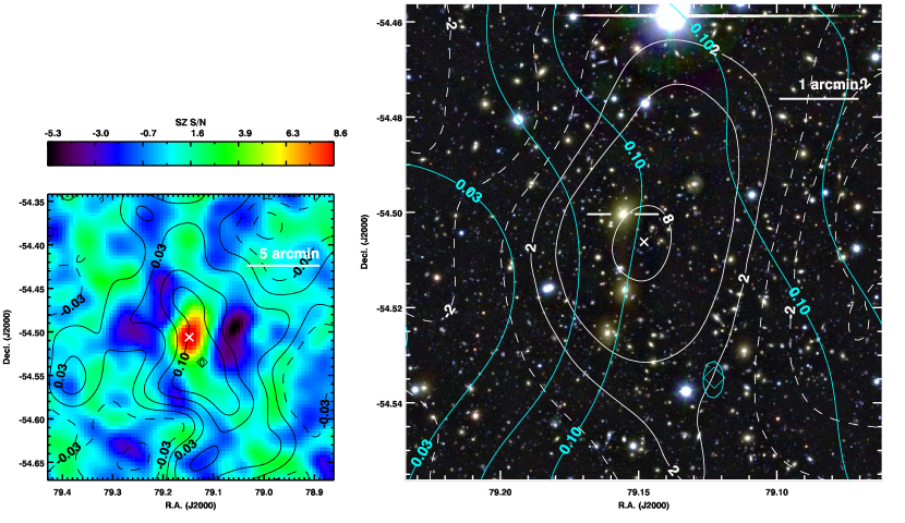
Figure 8.— SZ, optical, and $\kappa$ data for SPT-CL J0516-5430. See the Appendix for a description.

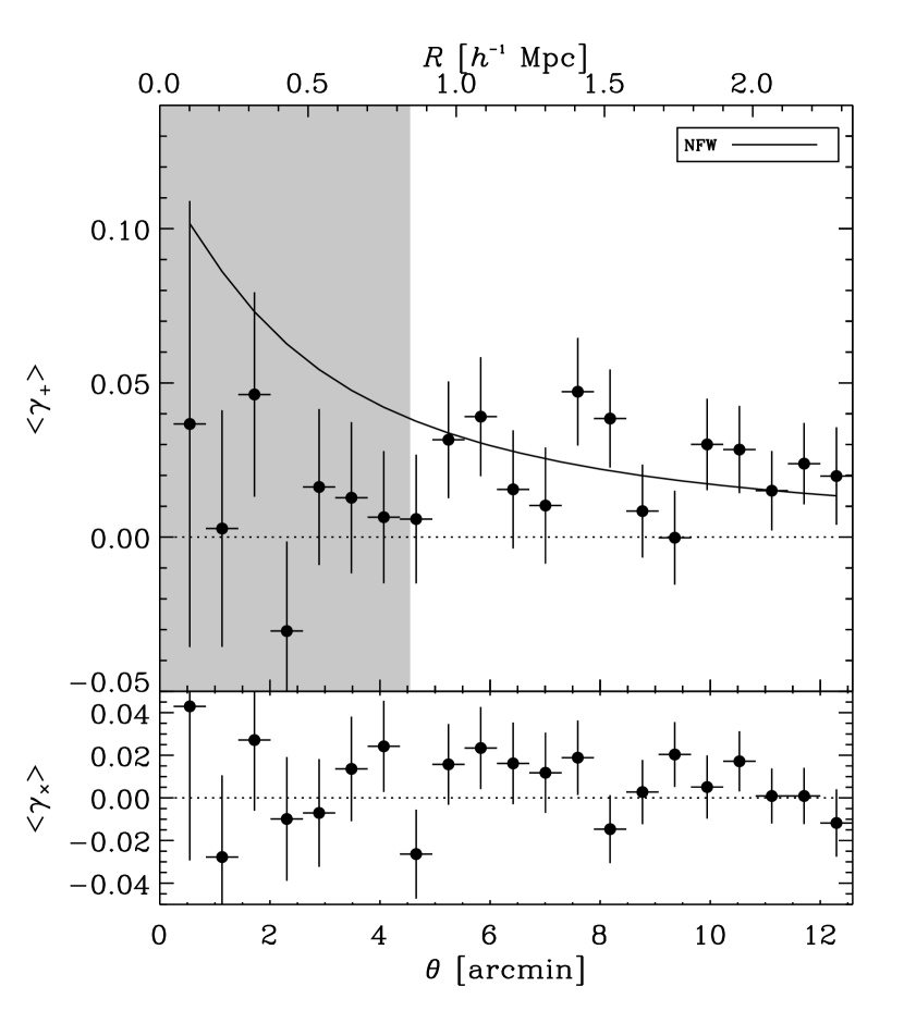
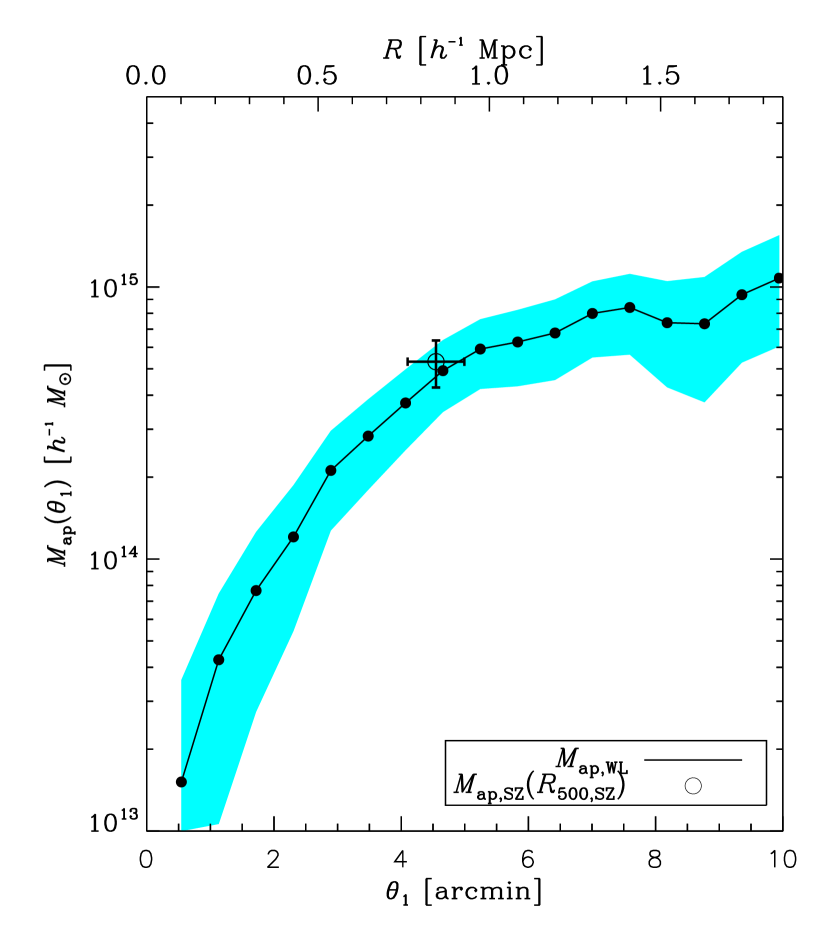
Figure 9.— Shear and aperture mass profiles of SPT-CL J0516-5430. See the Appendix for a description.

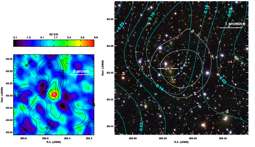
Figure 10.— SZ, optical, and $\kappa$ data for SPT-CL J2022-6323. See the Appendix for a description.

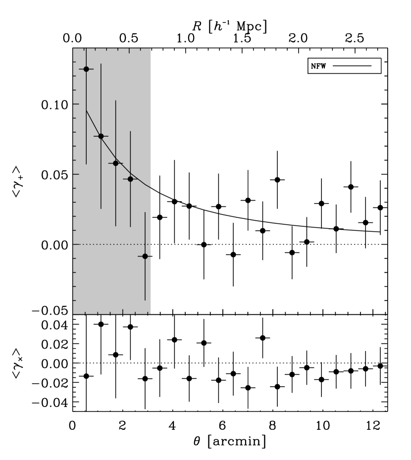
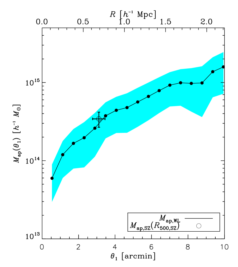
Figure 11.— Shear and aperture mass profiles of SPT-CL J2022-6323. See the Appendix for a description.

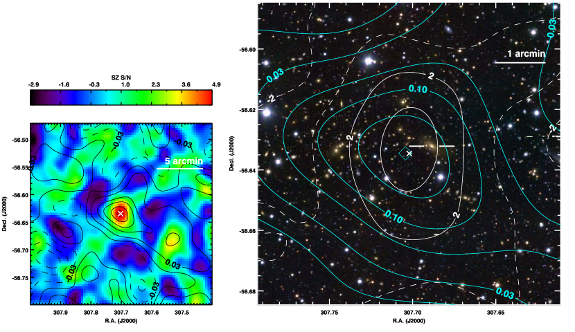
Figure 12.— SZ, optical, and $\kappa$ data for SPT-CL J2030-5638. See the Appendix for a description.

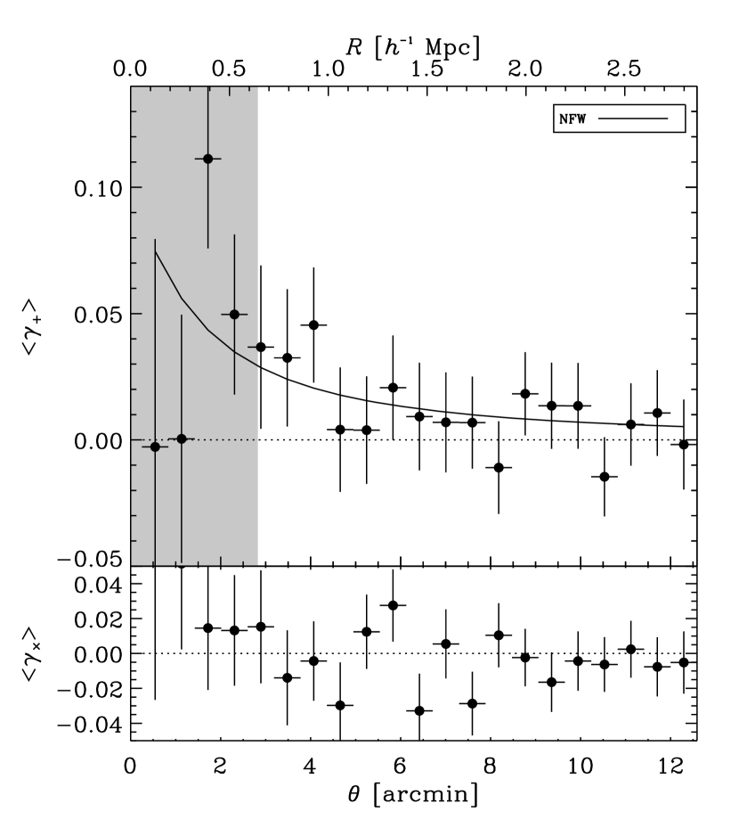
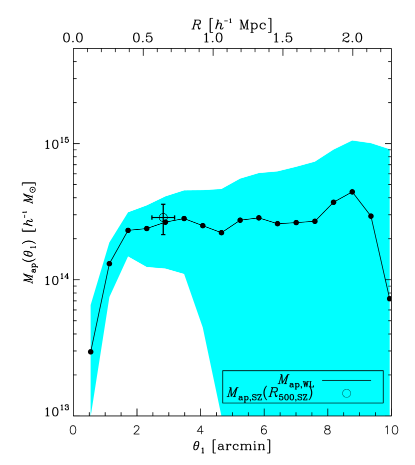
Figure 13.— Shear and aperture mass profiles of SPT-CL J2030-5638. See the Appendix for a description.

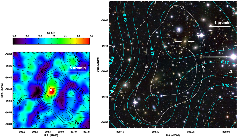
Figure 14.— SZ, optical, and $\kappa$ data for SPT-CL J2032-5627. See the Appendix for a description.

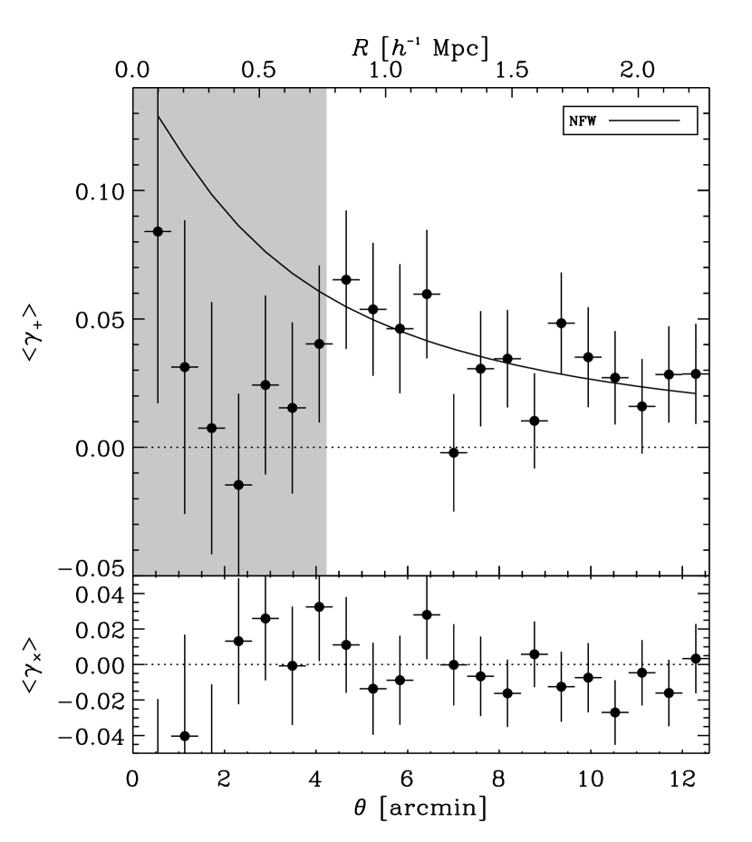
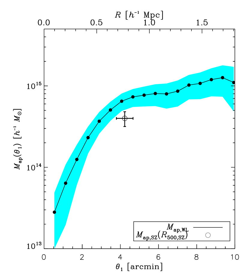
Figure 15.— Shear and aperture mass profiles of SPT-CL J2032-5627. See the Appendix for a description.

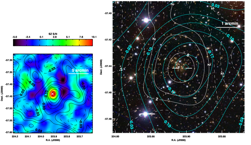
Figure 16.— SZ, optical, and $\kappa$ data for SPT-CL J2135-5726. See the Appendix for a description.

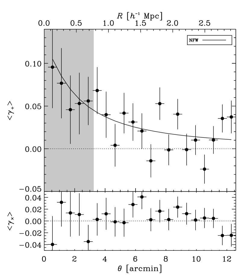
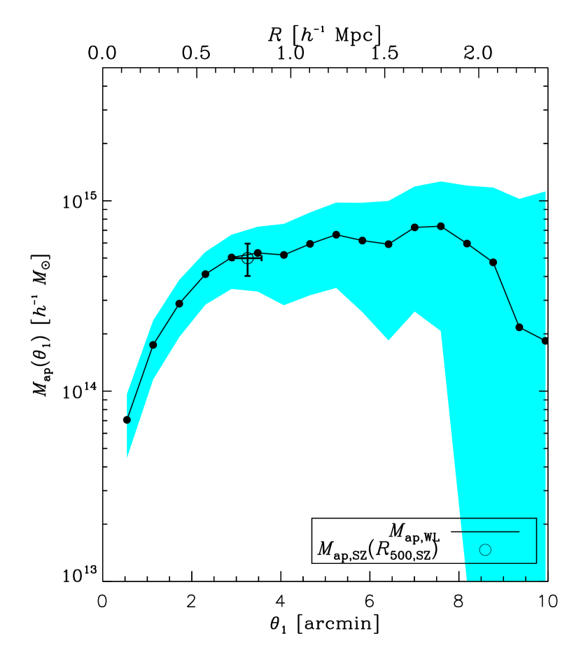
Figure 17.— Shear and aperture mass profiles of SPT-CL J2135-5726. See the Appendix for a description.

References

- Abell et al. (1989) Abell, G. O., Corwin, Jr., H. G., & Olowin, R. P. 1989, ApJS, 70, 1
- Albrecht et al. (2006) Albrecht, A., et al. 2006, ArXiv e-prints, astro-ph/0609591