Multimode circuit optomechanics near the quantum limit

The coupling of distinct systems underlies nearly all physical phenomena and their applications. A basic instance is that of interacting harmonic oscillators, which gives rise to, for example, the phonon eigenmodes in a crystal lattice. Particularly important are the interactions in hybrid quantum systems consisting of different kinds of degrees of freedom. These assemblies can combine the benefits of each in future quantum technologies. Here, we investigate a hybrid optomechanical system having three degrees of freedom, consisting of a microwave cavity and two micromechanical beams with closely spaced frequencies around 32 MHz and no direct interaction. We record the first evidence of tripartite optomechanical mixing, implying that the eigenmodes are combinations of one photonic and two phononic modes. We identify an asymmetric dark mode having a long lifetime. Simultaneously, we operate the nearly macroscopic mechanical modes close to the motional quantum ground state, down to 1.8 thermal quanta, achieved by back-action cooling. These results constitute an important advance towards engineering entangled motional states.

One of the present goals in physics is the explanation of macroscopic phenomena as emerging from the quantum-mechanical laws governing nature on a microscopic scale. This understanding is also important for future quantum information applications DeMille ; PainterRoute ; SembaQBspin ; KorppiPRL2011 , since many of the most promising platforms base on nearly macroscopic degrees of freedom. For macroscopic mechanical objects, their potential quantum behavior OConnell:2010br has been actively investigated with resonators interacting with an electromagnetic cavity mode KippenbergReview . In particular, freezing of the mechanical Brownian motion Metzger:2004ei ; Rocheleau:2010jd down to below one quantum of energy has recently been observed Teufel2011b ; AspelmeyerCool11 .

Another result of radiation-pressure interaction is the mixing of the normal modes of vibration into linear combinations of the uncoupled phonon and photon modes. This has been verified with optomechanical Fabry-Perot cavity Groeblacher:2009eh , and by its on-chip microwave analogy Teufel2011b using an aluminum membrane. All this work is paving the way towards engineering non-classical motional OConnell:2010br and hybrid quantum states DeMille ; LaHaye2009 ; SembaQBspin ; KorppiPRL2011 for basic tests of quantum theory Legget2002 ; MartinisBell , as well as applications in foreseeable future.

Corresponding phenomena in systems comprising of more than two active degrees of freedom KippenbergMulti ; MarquardtMulti have received less attention. In the optomechanical crystal setup, coupling of mechanical vibrations via radiation pressure interaction has been demonstrated with the zipper cavity PainterMix2010 , however, with some direct interaction between the beams. In the microwave regime, such measurements have remained outstanding. In this work, we take a step further, and examine a multimode system where two micromechanical beams, having resonant frequencies $\omega_{1}/(2\pi)=32.1$ MHz and $\omega_{2}/(2\pi)=32.5$ MHz, are each coupled to a microwave on-chip cavity. We obtain the first evidence of hybridization of all the three degrees of freedom. This was made possible by operating, as opposed to the optical setup, in the good-cavity limit, that is, both $\omega_{1}$ and $\omega_{2}$ were much larger than the cavity decay rate $\gamma_{c}$. Simultaneously, the mechanical modes are found at low occupation numbers $n_{m}$ near the quantum ground state, down to $n_{m}=1.8\pm 0.5$. These are the lowest occupation recorded with nanowire resonators to date, and they occur via the sideband cooling, starting from operation at dilution refrigerator temperatures at a few tens of mK.

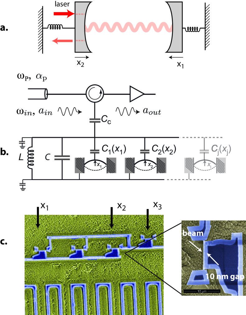
Figure 1: Cavity-controlled coupling of micromechanical resonators. a, Optomechanical system with both mirrors movable has three degrees of freedom. b, analogy of (a) with a microwave-regime cavity represented by the lumped element inductors and capacitors and arbitrary number $j=1...N$ of mechanical resonators. The experiments are performed by shining a strong pump microwave tone (frequency $\omega_{P}$), and possibly a weak probe tone (frequency $\omega_{\mathrm{in}}$) in a dilution refrigerator down to 25 mK temperature. c, images of the all-aluminum superconducting sample, showing four fabrication jigs for a beam. Total of three beams ($x_{1}...x_{3}$) were operating. Beams 1 and 2 had large electromechanical couplings $g_{1}/2\pi=1.8$ MHz/nm, $g_{2}/2\pi=2.0$ MHz/nm, whereas the third beam had an order of magnitude smaller coupling.

In the optical domain PainterMix2010 , a three-mode optomechanical system can be pictured as a Fabry-Perot cavity with both massive mirrors mounted via springs, see Fig. 1a. In the microwave version, (Fig. 1b), the mirrors are replaced by movable capacitors formed by the mechanical resonators. The electromechanical coupling arises when each mechanical resonator (labelled with $j$), expressed as time-varying capacitors $C_{j}$, independently modulates the total capacitance, and hence, the cavity frequency $\omega_{c}$. This is described by the coupling energies $g_{j}=(\omega_{c}/2C)\partial C_{j}/\partial x_{j}$.

In the actual device (see micrograph in Fig. 1c), the mechanical resonators are spatially separated by about 100 microns, and we hence expect the direct interaction between the beams via the substrate material to be negligible. We drive the cavity strongly by a microwave pump signal applied at the frequency $\omega_{P}$ near the cavity frequency. The pump induces a large cavity field with the number of pump photons $n_{P}\gg 1$. This allows for a linearized description of the electromechanical interaction and results in substantially enhanced effective couplings $G_{j}=g_{j}x_{0j}\sqrt{n_{P}}$.

Results

Cavity with several mechanical modes The general Hamiltonian for $N$ mechanical resonators with frequencies $\omega_{j}$, individually coupled to a common cavity mode, written in a frame rotating with the pump, becomes

$$H=-\hbar\Delta a^{\dagger}a+\hbar\sum_{j=1}^{N}\omega_{j}b_{j}^{\dagger}b_{j}-\hbar\left(a^{\dagger}+a\right)\sum_{j=1}^{N}G_{j}\left(b_{j}^{\dagger}+b_{j}\right)$$ (1)

Here, $a$ is the annihilation operator for the cavity mode, $b_{j}$ are those of the mechanical resonators, and $x_{0j}=\sqrt{\hbar/2m_{j}\omega_{j}}$ is the zero-point amplitude. If one assumes roughly similar mechanical resonators, viz.  $\omega_{j}\sim\omega_{m}$ and $G_{j}\sim G$, the cavity becomes nearly resonant to all of them at the red-sideband detuned pump condition $\Delta=-\omega_{m}$.

Coupling of the mechanical resonators via the cavity ”bus” can be anticipated to be significant if the mechanical spectra begin to overlap when their width increased by the radiation pressure, $\gamma_{\mathrm{eff}}=\gamma_{m}+\gamma_{\mathrm{opt}}$, grows comparable to the mechanical frequency spacing. Here, $\gamma_{\mathrm{opt}}=4G^{2}/\gamma_{c}$. The equations of motion following from Eq. (1) allow one to verify the above assumption. We will in the following focus on two resonators, $N=2$. The result of such calculation, which is detailed in the Supplementary Information, is that they experience an effective coupling with energy $G_{12}=G_{1}G_{2}/\gamma_{c}$.

In the limit of strong coupling, $\sqrt{(G_{1}^{2}+G_{2}^{2})/2}\gg\gamma_{c}/4$, the system is best described as a combination of two ”bright” modes with linewidths $\sim\gamma_{c}/2$, and of a ”dark” mode having a long lifetime $\sim\gamma_{m}$. In the latter, the two mechanical resonators oscillate out-of-phase and synchronize into a common frequency $(\omega_{1}+\omega_{2})/2$. In any case, the mode structure can be written with the normal coordinates for mode $n$, for position quadrature according to $X^{(n)}=D_{c}^{(n)}q_{c}+\sum_{j=1}^{N}D_{j}^{(n)}q_{j}$, and similarly for the momentum quadrature $P^{(n)}$.

In the experiment, we use doubly clamped flexural beams which are made by the use of ion beam milling of aluminum Sulkko:2010ih , having an ultranarrow $\sim 10$ nm vacuum slit to the opposite end of the cavity for maximizing the coupling. The cavity is $\lambda/2$ floating microstrip similar to Ref.  MechAmpPaper , resonating at $\omega_{c}/(2\pi)=6.98$ GHz. The total cavity linewidth $\gamma_{c}=\gamma_{E}+\gamma_{I}\simeq(2\pi)\times 6.2$ MHz is a sum of the internal damping $\gamma_{I}/(2\pi)=1.4$ MHz, and the external damping $\gamma_{E}/(2\pi)=4.8$ MHz. At at the highest powers discussed, however, we obtain a decreased $\gamma_{I}/(2\pi)=0.9$ MHz, typical of dielectric loss mechanism.

There are a total of three beams as shown in Fig. 1c. Two of the beams have a large zero-point coupling of $g_{1}x_{01}/2\pi=39$ Hz, and $g_{2}x_{02}/2\pi=44$ Hz. The frequencies of beams 1 and 2 were relatively close to each other, $\omega_{2}-\omega_{1}\sim(2\pi)\,450$ kHz, such that it is straightforward to obtain an effective coupling $G_{12}$ of the same order. The third beam had an order of magnitude smaller coupling, and hence we neglect it in the full calculation, setting $N=2$ in Eq. (1) in what follows.

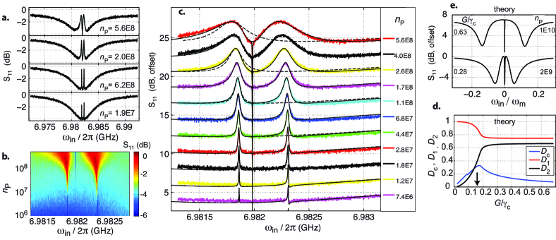
Figure 2: Hybridization of microwave photons and two radio-frequency phonons. a, Measured reflection coefficient of probe microwave while a strong pump is applied at the red sideband, $\Delta\simeq-\omega_{1}$, while increasing pump amplitude, from bottom to top. b, c, zoomed-in view of (a). An excellent agreement with the theory is obtained with reflection calculation using a complete model based on Eq. (1), for two beams 1 and 2 (solid lines). The dashed lines show a fit with an independent-resonator model for beam 1. The narrow feature at 6.982 GHz is due to beam 3. The curves are displaced vertically by 3 dB for clarity. d, normal modes of oscillations expressed as linear combinations of photon and two phonons for the dark mode. The parameters are as in c. The arrow denotes the highest experimental value. e, Theory plot for higher $n_{P}$; the dark mode is expected to become narrower and more and more phonon-like. Here, $\Delta=-(\omega_{1}+\omega_{2})/2$. For simplicity, we take $g^{(2)}_{j}=0$ in d and e.

The measurements are conducted in a cryogenic temperature below the superconducting transition temperature of the Al film ($\sim 1$ K) in order to reduce losses. We used a dilution refrigerator setup as in Ref. MechAmpPaper down to 25 mK, which allows for a low mechanical mode temperature in equilibrium. Apart from this, cryogenic temperatures or superconductivity are not necessary Weig2011 .

Experimental data The modes can be probed by adding to the experimental setup another, the probe, tone Groeblacher:2009eh ; Teufel:2011ha ; MechAmpPaper with frequency $\omega_{\mathrm{in}}$. The maximum pump power we can reach is $4\,\mu$W, inducing a coherent $n_{P}\sim 6\times 10^{8}$ photon occupancy in the cavity, and effective coupling $G_{12}=(2\pi)\times 150$ kHz (with $G_{1}=0.93$ MHz, $G_{2}=1.0$ MHz). In Fig. 2a, we display changes of the cavity absorption by increasing the pump power. The two peaks at the bottom of the cavity dip are due to the beams 1 and 2. They broaden with increasing $n_{P}$, finally leaving behind a narrow dip between them. The overall lineshape is clearly not a sum of two Lorentzian peaks.

In Fig. 2c we show a zoom-in view of the two peaks, together with theoretical predictions. One immediately sees that an attempt to simulate either peak by a single mechanical resonator coupled to cavity ($N=1$ in the analysis), thereby neglecting the cavity-mediated coupling, fails to explain the lineshape at large $n_{P}\gtrsim 10^{8}$. The full simulation with both beams 1 and 2 included, however, produces a remarkable agreement to the experiment. In order to create these curves, we further take into account a shift of the mechanical frequencies due to second-order interaction Rocheleau:2010jd , given as $-\frac{1}{2}g^{(2)}_{j}n_{P}$, where $g^{(2)}_{j}=x_{0j}^{2}\omega_{c}/2C\left(\partial^{2}C_{j}/\partial x^{2}_{j}\right)\sim(2\pi)\,3\times 10^{-4}$ Hz is the second-order coupling coefficient. The third beam, visible in Fig. 2c as a narrow feature just below 6.982 GHz, was later fitted by running a single-resonator calculation. This is justified because its mixing is negligible owing to weak coupling.

The narrow dip between the peaks manifests the onset of the dark mode, where the cavity participation approaches zero with growing $G_{j}$, as occurs also in other tripartite systems Tripartite . As usual for weakly decaying states, the dark modes can be useful for storage of quantum information EITrmp ; PainterMix2010 . The other two dips (best discerned in the theoretical plots at higher $G_{j}$, see Fig. 2e) are the bright modes, and they retain fully mixed character of all three degrees of freedom. In Fig. 2d we display the prediction for the mode expansion coefficients with respect to coupling. Asymmetry in the role of the mechanical modes is sensitive to parameters. With the maximum coupling in the experiment ($G_{j}/\gamma_{c}\simeq 0.15$), the normal modes are well mixed: the dark mode can be expressed as $\left[D_{c},D_{1},D_{2}\right]\sim\left[0.3,0.3,0.9\right]$.

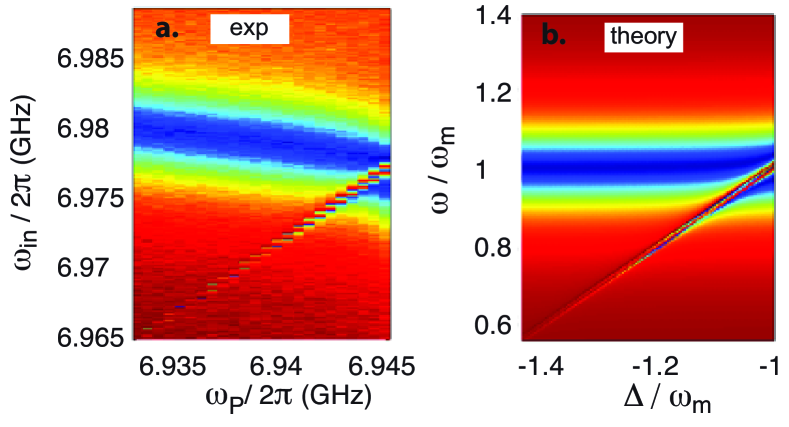
Figure 3: Pump detuning measurements. a, Measured spectrum of the tripartite cavity electromechanical system when pumped at a fixed input power such that at resonance, $\Delta\sim\left(-\omega_{1},-\omega_{2}\right)$, $n_{P}\simeq 5.6\times 10^{8}$. The pump frequency was slowly swept from left to right. b, theory prediction.

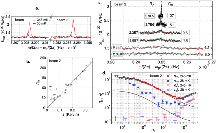
Figure 4: Sideband cooling of motion down to 1.8 thermal quanta. a, cavity output spectra representing the thermal motion peaks of beams 1 and 2 measured at 345 mK and 35 mK, with $n_{P}=4\times 10^{5}$. b, calibration of the detection according to temperature dependence of the mechanical energy $n_{m}\hbar\omega_{m}=k_{B}T$, given by the area of the peak (data for beam 2). c, output spectra of beam 2 at pump occupation $n_{P}$ increasing from top to bottom. The curves are shifted vertically by 0.3 y-axis units for clarity. The corresponding mechanical occupations are written on the right. d, progress of back-action cooling (beam 2) as a function of pump occupation. The mechanical mode temperature is given by circles, and the cavity temperature by squares. Red: high temperature, 245 mK; blue, base temperature (28 mK). The ideal theoretical behavior are plotted by the solid lines. Unless the data point for $n_{c}^{T}$, including its error bars, was of positive sign, only the absolute value of the error bar is plotted.

One can also vary the pump detuning, thereby effectively detuning the cavity and the mechanical resonators Groeblacher:2009eh ; Teufel:2011ha . An anticrossing of the cavity and mechanical modes is seen in Fig. 3a up to detuning $\Delta\sim-\omega_{m}$, above which the system exhibits parametric oscillations. The pertinent simulation, Fig. 3b, portrays the main features of the measurement, except bending of the cavity frequency towards lower value in an upward sweep of $\Delta$. We expect such possibly hysteretic behavior of the cavity frequency to be due to second-order effects beyond the present linear model.

Sideband cooling We now turn the discussion into showing how the tripartite system resides nearly in a pure quantum state during the mode mixing experiments. The mechanical resonators can be sideband-cooled with the radiation pressure back-action Regal:2008di ; Kippenberg2009 ; Hertzberg:2010 ; Rocheleau:2010jd under the effect of the pump which also creates the mode mixing. Although the ground state of one mode was recently achieved this way Teufel2011b ; AspelmeyerCool11 , cooling in multimode or nanowire systems is less advanced.

The incoherent output spectrum can be due to either a finite phonon number $n_{m}$, or non-equilibrium population number $n_{c}^{T}$ of the cavity. The former manifests as a Lorentzian centered at the upper sideband, as in Fig. 4a, with the linewidth $\gamma_{\mathrm{eff}}=\gamma_{m}+4G^{2}/\gamma_{c}$, whereas the latter gives a small emission at broader bandwidth. The analytical theory Rocheleau:2010jd and experimental details are discussed in Supplementary Information.

At low input power, when the cavity back-action damping is small and $n_{c}^{T}\sim 0$, phonon number is set by thermal equipartition $n_{mj}\hbar\omega_{j}=k_{B}T$. This is best observed by the area of the mechanical peak in the output spectrum, as in Fig. 4a, which should be linear in cryostat temperature. The linearity holds down to about 150 mK temperatures (Fig. 4b), below which we observe intermittent heating which is sensitive to parameters.

The resulting cooling of beam 2 is displayed in Fig. 4d. At a relatively high temperature of 245 mK, the data points follow theory well up to input powers corresponding to $n_{P}\sim 5\times 10^{7}$. At the minimum cryostat temperature of 28 mK, the mode is not thermalized in a manner which depends irregularly on power. We obtain a minimum phonon number $n_{m2}\sim 1.8$, where the mechanical mode spends one third of the time in the quantum ground state. The other mechanical mode, beam 1, cooled simultaneously down to 2.5 quanta, possibly compromised by the slightly smaller coupling. The cooling is quite clearly bottlenecked by heating, by the pump microwave, of the bath to which the mechanical mode is coupled. For the optimum data points, the starting temperature for cooling has raised to 150 mK, and above this it grows roughly quadratically with $n_{P}$.

Discussion

The coupling of micromechanical resonators mediated via microwave photons in an on-chip cavity is a basic demonstration of the control of a multimode mechanical system near the quantum limit. The setup provides a flexible platform for creation and studies of nonclassical motional states entangled over the chip OptoEntang , or over macroscopic distances AspelmeyerPRL07 ; ligo . The setup is easily extended to embody nearly arbitrarily many mechanical resonators, hence allowing for designing an electromechanical metamaterial with microwave-tunable properties. For future quantum technology applications even at elevated temperatures Weig2011 , data may be stored Painter2011 in weakly decaying dark states identified in the present work.

Methods

Device fabrication

The lithography to define the meandering cavity and jigs for the beams consisted of a single layer of electron-beam exposure, followed by evaporation of 150 nm of aluminum on a fused silica substrate. Since the cavity is of planar structure, it has no potentially problematic cross-overs which tend to have weak spots in superconducting properties and hence could heat up the cavity. We thus expect the cavity to portray a high critical current limited only by the intrinsic properties of the strip. With a 2 $\mu$m wide strip, we expect the critical current to be several mA. With the maximum circulating currents in cavity (Fig. 2), about 0.5 mA of peak value, there was no sign of nonlinearity in the cavity response.

The mechanical resonators were defined by Focused Ion Beam (FIB) cutting, as in Ref. Sulkko:2010ih . We used low gallium ion currents of 1.5 pA which gives the nominal beam width of about 7 nm. In order to maximize sputtering yield with minimal gallium contamination, we used a single cutting pass mode. Otherwise, the cut beams tend to collapse to the gate. With the current recipe, fabrication of down to 10 nm gap widths over 5-10 microns distance can be done with about 50 % yield.

Theory of cavity-coupled resonators

The Hamiltonian for $N$ mechanical resonators each coupled to one cavity mode via the radiation pressure interaction is

$$H=\hbar\omega_{c}a^{\dagger}a+\hbar\sum_{j=1}^{N}\omega_{j}b_{j}^{\dagger}b_{j}-\hbar a^{\dagger}a\sum_{j=1}^{N}g_{j}x_{0j}\left(b_{j}^{\dagger}+b_{j}\right)+H_{P}$$ (2)

The pump with the Hamiltonian $H_{P}=2\hbar\sqrt{\frac{P_{P}\gamma_{E}}{\hbar\omega_{c}}}\left(a^{\dagger}+a\right)\cos{\omega_{P}t}$ induces a large cavity field with the number of pump photons $n_{P}\gg 1$.

Under the strong driving, the cavity-mechanics interaction can be linearized individually for each beam, resulting in Eq. (1). Further details of the calculations are given in the Supplementary Information.

Sideband cooling

For one beam, the measured output spectrum divided by system gain, $S_{\mathrm{out}}(\omega)$, carries information on the phonon number according to Rocheleau:2010jd

$$S_{\mathrm{out}}=\frac{\gamma_{E}}{\gamma_{c}}n_{c}^{T}+\frac{\gamma_{E}}{\gamma_{c}}\gamma_{\mathrm{opt}}\frac{\gamma_{\mathrm{eff}}}{\left(\omega-\omega_{m}\right)^{2}+\gamma_{\mathrm{eff}}^{2}/4}\left(n_{m}-2n_{c}^{T}\right)$$ (3)

which is a Lorentzian centered at the cavity frequency. A non-zero base level is due to possible broadband emission from the cavity, due to a thermal state with occupation $n_{c}^{T}$. We suppose that at modest pump (cooling) powers of utmost interest, coupling of the mechanical resonators remains insignificant, and thus we can apply Eq. (3) separately for each resonator. Some deviations can, however, occur at the highest powers with $n_{P}\sim 3\times 10^{8}$.

In order to obtain the phonon number under strong back-action, we fit a Lorentzian to each peak as in Fig. 4c, obtaining independently the base level, amplitude and linewidth for every input power. These values are then compared to Eq. (3). This leaves, however, yet too many unknowns in order to obtain the occupations of the mechanics and cavity. This is basically because of uncertainties in the attenuations of both input and amplifier lines, which limit the accuracy of estimating $n_{P}$. We can obtain a calibration using the linear temperature dependence, and by fitting the dependence of $\gamma_{\mathrm{eff}}$ on input power.

As opposed to for instance to Ref. Rocheleau:2010jd , the bottleneck for cooling is not heating of the cavity by strong pump, as seen in Fig. 4d, where the cavity temperature is increasing only little up to the optimum cooling powers corresponding to about 0.15 mA of peak current values in cavity. This can be due to the simplistic structure of the cavity.

The above analysis supposes the presence of nearly no non-equilibrium photons in the cavity at zero or low input powers. This situation can be investigated by observing a possible emission from about cavity linewidth under these conditions. A complication arises because the cavity linewidth is so large such that a small change is easily overwhelmed by modest standing waves in cabling. We avoided this issue by using temperature dependence of the cavity frequency, due to the kinetic inductance in the long microstrip. Thereby, a broad emission peak moving according to the cavity frequency would be easily distinguishable. We observed no such signal down to the level of $n_{P}^{T}\lesssim 0.1$ which justifies the above analysis.

Acknowledgements We would like to thank S. Paraoanu and Lorenz Lechner for useful discussions. This work was supported by the Academy of Finland, by the European Research Council (grants No. 240362-Heattronics and 240387-NEMSQED), and by the Vaisala Foundation.

Multimode circuit optomechanics near the quantum limit: Supplementary information

Francesco Massel¹, Sung Un Cho¹, Juha-Matti Pirkkalainen¹, Pertti J. Hakonen¹, Tero T. Heikkilä¹, and Mika A. Sillanpää¹

¹Low Temperature Laboratory, Aalto University, P.O. Box 15100, FI-00076 AALTO, Finland

I Response of coupled resonators

We detail here the theory of the response of a driven cavity coupled to $N$ (with emphasis on the case $N=2$) mechanical resonators. In particular, we show how it is possible to describe the system from two complementary points of view. On one hand, the cavity-mechanics interaction provides a dressing of the dynamics of the resonators, leading to the definition of effective mechanical frequencies and dampings. On the other hand, for strong coupling, we find that on top of the normal mode splitting found for single resonators, the system exhibits a dark mode which gets asymptotically decoupled from the cavity, and whose linewidth tends to the bare linewidth of the mechanical resonances.

We define the following symbols: The mechanical resonators have frequencies $\omega_{j}$ and linewidths $\gamma_{j}$. Their annihilation operators are denoted by $b_{j}$ while $q_{j}=\frac{1}{\sqrt{2}}\left(b_{j}^{\dagger}+b_{j}\right)$ and $p_{j}=\frac{i}{\sqrt{2}}\left(b_{j}^{\dagger}-b_{j}\right)$ are the dimensionless amplitude and momentum of the mechanical oscillations. The mechanical zero-point amplitude is $x_{0j}=\sqrt{\hbar/2m_{j}\omega_{j}}$. Correspondingly, the cavity has the frequency $\omega_{c}$ and linewidth $\gamma_{c}=\gamma_{E}+\gamma_{I}$, consisting of the external and internal dissipation, respectively. $a$ is the annihilation operator for the cavity. The pump microwave (applied at the frequency $\omega_{P}$ near the cavity frequency) has the detuning from the cavity $\Delta=\omega_{P}-\omega_{c}$, and the power $P_{P}$.

The Hamiltonian for $N$ mechanical resonators each coupled to one cavity mode via the radiation pressure interaction is

$$H=\hbar\omega_{c}a^{\dagger}a+\hbar\sum_{j=1}^{N}\omega_{j}b_{j}^{\dagger}b_{j}-\hbar a^{\dagger}a\sum_{j=1}^{N}g_{j}x_{0j}\left(b_{j}^{\dagger}+b_{j}\right)+H_{P}$$ (4)

The pump with the Hamiltonian $H_{P}=2\hbar\sqrt{\frac{P_{P}\gamma_{E}}{\hbar\omega_{c}}}\left(a^{\dagger}+a\right)\cos{\omega_{P}t}$ induces a large cavity field with the number of pump photons $n_{P}\gg 1$. The number of quanta the in cavity due to pump is

$$n_{P}=\frac{P_{P}\gamma_{E}}{\hbar\omega_{c}}\frac{1}{\Delta^{2}+\left(\frac{\gamma}{2}\right)^{2}}$$ (5)

where angular frequency units are used.

The equations of motion following from the Hamiltonian, Eq. (1) in the main text, linearized about a steady-state, can be written as masselsuppl

$$\dot{a} =i\Delta a-\frac{\gamma_{c}}{2}a+i\sum_{j=1}^{N}G_{j}q_{j}+\sum_{i=I,E}\sqrt{\gamma_{i}}a^{i}_{\rm in}$$ (6)

$$\dot{q}_{j} =\omega_{j}p_{j}$$ (7)

$$\dot{p}_{j} =-\omega_{j}q_{j}-\gamma_{j}p_{j}+G_{j}\left(a^{\dagger}+a\right)+\xi_{j},$$ (8)

where $a_{\rm in}^{i}$ are input fields to the cavity ($I$ and $E$ denoting internal and external input fields, the previous describing internal dissipation and the latter the coupling to the measurement setup), and $\xi_{j}$ are fields driving the mechanical resonators. Moreover, $G_{j}=\sqrt{n_{P}}g_{j}$ describes the cavity driving (by photon number $n_{P}$) enhanced coupling between the cavity field and resonator $j$. Fourier transforming and, after some algebra, assuming a probe field $a_{\rm in}=a_{\rm in}^{E}$ and neglecting the noise terms $\xi_{j}$ yields

$$X\equiv a^{\dagger}+a=\tilde{\chi}\left(\omega\right)\sum_{j=1}^{N}G_{j}q_{j}-i\sqrt{\gamma_{E}}\left[\chi_{-\Delta}\left(\omega\right)a_{\rm in}+\chi_{\Delta}\left(\omega\right)a_{\rm in}^{\dagger}\right]$$ (9)

$$q_{j}=\chi_{j}(\omega)G_{j}X$$ (10)

where the response functions are

$$\chi_{\Delta}(\omega)=\frac{1}{\Delta-\omega-i\gamma_{c}/2},\quad\chi_{j}(\omega)=\frac{\omega_{j}}{\omega_{j}^{2}-\omega^{2}-i\gamma_{j}\omega}$$ (11)

and

$$\tilde{\chi}(\omega)=\chi_{-\Delta}(\omega)-\chi_{\Delta}(\omega)=\frac{2\Delta}{(\omega+i\gamma_{c}/2)^{2}-\Delta^{2}}.$$ (12)

Solving for $X$, we get

$$X=\sqrt{\gamma_{E}}M(\omega)\left[\chi_{-\Delta}a_{\rm in}+\chi_{\Delta}a_{\rm in}^{\dagger}\right]$$ (13)

with

$$M(\omega)=\frac{1}{1-\tilde{\chi}(\omega)\sum_{j=1}^{N}G_{j}^{2}\chi_{j}(\omega)}.$$ (14)

This field is coupled to the cavity output field by

$$a_{\rm out}^{(\dagger)}=\sqrt{\gamma_{E}}a^{(\dagger)}-a_{\rm in}^{(\dagger)}.$$ (15)

When the effect of $a_{\rm in}^{\dagger}$ on $a$ can be disregarded (see below), we can write $a_{\rm out}=R(\omega)a_{\rm in}$, where $R(\omega)=-i\gamma_{E}M(\omega)\chi_{-\Delta}(\omega)-1$ is the reflection probability amplitude in the cavity. Figure 2 of the main text shows its absolute value, corresponding to the measured observable.

The effective dynamics of the system is qualitatively different in different regimes. For typical structures $\gamma_{c}\gg\gamma_{j}$. In this case, when $G_{1}^{2}+G_{2}^{2}\ll(\gamma_{c}/4)^{2}$, the cavity response $\tilde{\chi}(\omega)$ is approximatively independent of frequency within the relevant frequencies describing the mechanics. In this case, we can view the system as two mechanical resonators effectively coupled by the cavity (Sec. I.1). On the other hand, for large $G_{j}$ (sec. IB), the normal modes of the total system split. There are two bright modes strongly coupled to the cavity, with resonance frequencies $\omega_{b}\approx\Delta\pm\sqrt{\sum_{j}G_{j}^{2}}$ and linewidths $\sim\gamma_{c}/2$, and one “dark” mode at around $(\omega_{1}+\omega_{2})/2$ and with a linewidth $\sim\gamma_{j}$. The latter is almost decoupled from the cavity, with the coupling decreasing with an increasing $G_{j}$.

I.1 Weak-coupling regime

In the following, we concentrate on the case of red-detuned driving, $\Delta\approx-\omega_{j}$ in the sideband resolved case $\gamma_{c}\ll\omega_{j}$, and study the response at frequencies $\omega\approx-\Delta$. This allows us to approximate

$$\chi_{j}(\omega)\approx\frac{1}{2(\omega_{j}-\omega)-i\gamma_{j}},\quad\tilde{\chi}\approx\frac{1}{\omega+\Delta+i\gamma_{c}/2}.$$ (16)

The same approximation yields $\chi_{\Delta}(\omega)\ll\chi_{-\Delta}(\omega)$ and we may hence disregard the input field $a_{\rm in}^{\dagger}$ at these frequencies.

Let us restrict to the case of two mechanical resonators. Then the response function $M(\omega)$ may be written in the form

$$M(\omega)= \frac{\left(\omega_{1}-\omega-i\gamma_{1}/2\right)\left(\omega_{2}-\omega-i\gamma_{2}/2\right)}{\left(\omega_{1}-\omega-i\gamma_{1}/2\right)\left(\omega_{2}-\omega-i\gamma_{2}/2\right)-\tilde{\chi}(\omega)\left[G_{1}^{2}\left(\omega_{2}-\omega-i\gamma_{2}/2\right)+G_{2}^{2}\left(\omega_{1}-\omega-i\gamma_{1}/2\right)\right]/2}$$

$$\equiv \frac{\left(\omega_{1}+\omega-i\gamma_{1}/2\right)\left(\omega_{2}+\omega-i\gamma_{2}/2\right)}{\left(\omega_{1}^{c}+\omega-i\gamma_{1}^{c}/2\right)\left(\omega_{2}^{c}+\omega-i\gamma_{2}^{c}/2\right)}$$ (17)

We return to the definition of $\omega_{j}^{c}$ and $\gamma_{j}^{c}$ below, but now we rewrite the response in a more compact form

$$X=\frac{\chi_{1}^{c}}{\chi_{1}}\frac{\chi_{2}^{c}}{\chi_{2}}\chi_{-\Delta}\sqrt{\gamma_{E}}a_{\rm in}$$ (18)

$$q_{1}=G_{1}\frac{\chi_{2}^{c}}{\chi_{2}}\chi_{1}^{c}\chi_{-\Delta}\sqrt{\gamma_{E}}a_{\rm in}$$ (19)

$$q_{2}=G_{2}\frac{\chi_{1}^{c}}{\chi_{1}}\chi_{2}^{c}\chi_{-\Delta}\sqrt{\gamma_{E}}a_{\rm in},$$ (20)

where $\chi_{j}^{c}=\chi_{j}(\omega_{j}\mapsto\omega_{j}^{c})$. This form is readily generalized for more than two mechanical resonators. We now calculate $\omega_{j}^{c}$ and $\gamma_{j}^{c}$. For the sake of compactness, we include the broadening to the frequencies, allowing them to assume complex values

$$\omega_{j}\equiv\omega_{j}-i\gamma_{j}/2.$$ (21)

The frequencies $\omega_{1}^{c}$, $\omega_{2}^{c}$ appearing in the denominator of Eq. (17) can be expressed as

$$\omega_{1,2}^{c}=\frac{1}{2}\left[\omega_{1}^{e}+\omega_{2}^{e}\pm\sqrt{\left(\omega_{1}^{e}-\omega_{2}^{e}\right)^{2}+\tilde{\chi}(\omega)^{2}G_{1}^{2}G_{2}^{2}}\right]$$ (22)

where

$$\omega_{j}^{e}=\omega_{j}-\tilde{\chi}(\omega)G_{j}^{2}/2$$ (23)

are the effective frequencies (and dampings) of the mechanical resonators induced by the presence of the cavity, in the absence of the other mechanical resonator. The frequencies (and dampings) $\omega_{j}^{c}$ are thus the dressed mechanical frequencies in the presence of the cavity-mediated coupling between the mechanical resonators. Equation (22) describes an avoided crossing of the two mechanical resonators coupled by the energy

$$G_{12}\equiv\frac{1}{2}G_{1}G_{2}i\tilde{\chi}(\omega)\approx\frac{G_{1}G_{2}}{\gamma_{c}}.$$ (24)

The latter form is valid in the limit $\omega_{j}^{c}+\Delta\ll\gamma_{c}$, where we can approximate $\tilde{\chi}\approx-2i/\gamma_{c}$. For strong coupling or large initial frequency difference, the determination of $\omega_{1,2}^{c}$ requires the solution of Eq. (22) with the replacement $\tilde{\chi}(\omega)\to\tilde{\chi}(\omega_{1,2}^{c})$. The solutions of such a calculation are shown in Fig. 5, plotting the resulting frequency shifts and changes in the damping.

When $G_{12}\ll\omega_{1}^{e}-\omega_{2}^{e}$, we can disregard the coupling between the mechanical resonators, and the response of the cavity is a simple product of the individual responses. In the experiments, we reach $G_{12}=(2\pi)\times 150$ kHz (with $G_{1}=0.93$ MHz, $G_{2}=1.0$ MHz), which is roughly one third of the frequency difference between the mechanical resonators, and allows for the coupling effect to show up in the shape of the response curves. This is shown in Fig. 6, which compares the coupled response to the case of individual resonators.

Although the dressed response is affected by the coupling, the frequency shifts are not easily observed from the cavity response as they tend to be overwhelmed by the growing width $\sim{\rm Im}(\omega_{j}^{c})$. However, the frequency shifts can be seen in the mechanical response $q(\omega)/a_{\rm in}$, plotted in Fig. 7.

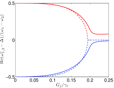
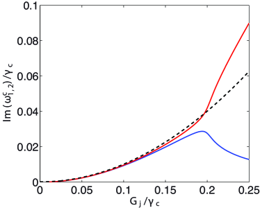
Figure 5: Values of $\omega_{1}^{c}$, $\omega_{2}^{c}$ in the weak-coupling regime. Left: real part of the frequencies and right: effective damping. On the left, the dashed lines show the approximation with a frequency independent coupling $G_{12}$ and disregarding the optical spring effect (Eq. (23)), whereas on the right, the dashed line shows the imaginary part of the effective frequencies $\omega_{j}^{e}$. For the damping, the coupling between the resonators shows up only in the strong-coupling regime. Here and in Figs. 7-8 the curves have been calculated with $\Delta=5\gamma_{c}$, $\omega_{1,2}=|\Delta|\pm 0.0075\Delta$ and $\gamma_{1}=\gamma_{2}=3\times 10^{-5}|\Delta|$, close to the experimental values, and for simplicity assuming $G_{1}=G_{2}$.

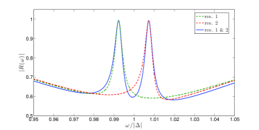
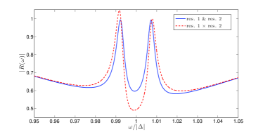
Figure 6: (left)Comparison of the reflection probability $|R(\omega)|$ for a single oscillator vs. that of two oscillators. (right) Comparison of the reflection probabilities when including (solid line, calculated with $\omega_{j}^{c}$) or excluding (dashed line, with $\omega_{j}^{e}$) the coupling induced normalization of the frequencies ($G=0.1\gamma_{c}$).

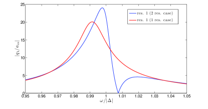
Figure 7: Mechanical spectrum of $|q_{1}|$ in the case of two (blue line) and one (red line) mechanical resonators, showing the frequency shift due to the coupling with the other resonator, an analogous situation would be observed for $|q_{2}|$ ($G=0.1\gamma_{c}$).

I.2 Strong-coupling regime

In the strong-coupling limit $\tilde{\chi}G_{1}^{2}G_{2}^{2}\gtrsim(\omega_{1}^{e}-\omega_{2}^{e})^{2}$, $\omega_{1,2}^{c}$ can be expressed as

$$\omega_{1,2}^{c}=\frac{1}{2}\left[\omega_{1}+\omega_{2}-\tilde{\chi}\left(\ G_{1}^{2}+G_{2}^{2}\right)/2\pm\sqrt{\tilde{\chi}^{2}\left(G_{1}^{2}+G_{2}^{2}\right)^{2}/4}\right],$$ (25)

from which we obtain two equations for $\omega_{1}^{c}$ and $\omega_{2}^{c}$

$$\omega_{1}^{c} =\frac{\omega_{1}+\omega_{2}}{2}+\tilde{\chi}(\omega_{1}^{c})\left(G_{1}^{2}+G_{2}^{2}\right)/2$$ (26)

$$\omega_{2}^{c} =\frac{\omega_{1}+\omega_{2}}{2}.$$ (27)

The second equation defines an asymptotic dark mode residing at the frequency between the two mechanical frequencies, and having a damping $(\gamma_{1}+\gamma_{2})/2$, i.e., typically much lower than that of the other dressed modes. For the first equation we have to include the full frequency dependence of $\tilde{\chi}(\omega)$ from Eq. (16). Multiplying the equation by $\tilde{\chi}^{(-1)}$ then yields another second-order equation for $\omega_{1}^{c}$, with the roots

$$\omega_{1}^{c}=\frac{1}{4}\left(-2\Delta+\omega_{1}+\omega_{2}+i\gamma_{c}\pm\sqrt{\left(-i\gamma_{c}+2\Delta+\omega_{1}+\omega_{2}\right){}^{2}+8G_{1}^{2}+8G_{2}^{2}}\right).$$ (28)

For simplicity, we consider in the following the case $\Delta=-(\omega_{1}+\omega_{2})/2$ which simplifies the expression to

$$\omega_{1}^{c}=-\Delta+\frac{1}{4}\left(i\gamma_{c}\pm\sqrt{8(G_{1}^{2}+G_{2}^{2})-\gamma_{c}^{2}}\right).$$ (29)

When $G_{1}^{2}+G_{2}^{2}>\gamma_{c}^{2}/8$, the real part of the frequencies tends to

$$\omega_{1}^{c}\rightarrow-\Delta\pm G,$$ (30)

where $G=\sqrt{(G_{1}^{2}+G_{2}^{2})/2}$. Moreover, the linewidth of these modes, whenever $G>\gamma_{c}/4$, is given by $\gamma_{c}/2$. In this case these frequencies and linewidths can be seen in the cavity response, as the cavity response function $|R(\omega)|$ has three dips: the outer dips, of width $\sim\gamma_{c}/2$ correspond to the (bright) modes $\omega_{1}^{c}$, whereas the inner narrow dip corresponds to the (dark) mode $\omega_{2}^{c}$ (see Fig. 2e of the main text).

Let us try to understand these modes from starting the equations of motion by redefining the mechanical motion to relative and center of mass motion (weighted by the couplings $G_{j}$), i.e.,

$$q_{a}=\left(G_{2}q_{1}-G_{1}q_{2}\right)/\left(G_{2}+G_{1}\right)$$ (31)

$$q_{s}=\left(G_{1}q_{1}+G_{2}q_{2}\right)/\left(G_{2}+G_{1}\right).$$ (32)

Below, we show that in the strong-coupling limit the above frequency $\omega_{2}^{c}$ describes the “dark” mode $q_{a}$ and the two frequencies $\omega_{1\pm}^{c}$ the “bright” modes $q_{s}$.

The equations of motion for these modes are

$$\dot{a} =i\Delta a+i(G_{1}+G_{2})q_{s}+\sqrt{\gamma_{E}}a_{\rm in}$$ (33a)

$$\dot{q}_{s} =\omega_{\Sigma}p_{s}+\omega_{\Delta}p_{a}$$ (33b)

$$\dot{q}_{a} =\omega_{\Sigma}p_{a}+\omega_{\Delta}p_{s}$$ (33c)

$$\dot{p}_{s} =-\omega_{\Sigma}q_{s}+\omega_{\Delta}q_{a}-\gamma p_{s}+\frac{G_{1}G_{2}}{G_{1}+G_{2}}\left(a^{\dagger}+a\right)$$ (33d)

$$\dot{p}_{a} =-\omega_{\Sigma}q_{a}+\omega_{\Delta}q_{s}-\gamma p_{a}$$ (33e)

with $\omega_{\Sigma}=\left(\omega_{1}+\omega_{2}\right)/2$ and $\omega_{\Delta}=\left(\omega_{1}-\omega_{2}\right)/2$. We have assumed that the linewidths of the two mechanical resonators are the same. If there is no frequency mismatch, the symmetric and antisymmetric modes are uncoupled.

Solving Eqs. (33), or substituting Eqs. (19,20) into (31) (and using the complex frequency notation) we obtain, in the strong-coupling limit

$$q_{s} =\frac{4G_{1}G_{2}}{\left(G_{2}+G_{1}\right)}\frac{\omega-\omega_{\Sigma}}{\left(\omega-\omega_{1+}^{c}\right)\left(\omega-\omega_{1-}^{c}\right)\left(\omega-\omega_{2}^{c}\right)}\sqrt{\gamma_{E}}a_{\rm in}$$ (34)

$$q_{a} =\frac{4G_{1}G_{2}}{\left(G_{2}+G_{1}\right)}\frac{\omega_{\Delta}}{\left(\omega-\omega_{1+}^{c}\right)\left(\omega-\omega_{1-}^{c}\right)\left(\omega-\omega_{2}^{c}\right)}\sqrt{\gamma_{E}}a_{\rm in}.$$ (35)

Considering that $\omega_{2}^{c}=\omega_{\Sigma}$, and assuming for simplicity $G_{1}=G_{2}\equiv G$, we have, when $\omega\simeq\omega_{1\pm}^{c}$,

$$q_{s+} =\frac{\sqrt{\gamma_{E}}}{(\omega-\omega_{1+}^{c})}a_{\rm in}$$ (36)

$$q_{s-} =-\frac{\sqrt{\gamma_{E}}}{(\omega-\omega_{1+}^{c})}a_{\rm in}$$ (37)

the cavity field becomes

$$X=\frac{\sqrt{\gamma_{E}}}{2(\omega-\omega_{1\pm}^{c})}a_{\rm in}.$$ (38)

Analogously, when $\omega\simeq-\Delta$, we get for $q_{a}$

$$q_{a}=\frac{2\omega_{\Delta}}{G\left(\omega-\omega_{2}^{c}\right)}\sqrt{\gamma_{E}}a_{\rm in}.$$ (39)

In this case the cavity field around the dark mode resonance frequency becomes

$$X=-\frac{\left(\omega_{1}+\Delta\right)\left(\omega_{2}+\Delta\right)}{G^{2}\left(\Delta-\omega_{2}^{c}\right)}\sqrt{\gamma_{E}}a_{\rm in}.$$ (40)

From Eq. (39) we see that, in the strong coupling limit, the mechanical mode $q_{a}$ is asymptotically decoupled from the input as well as from the cavity field, allowing to identify this mode as a dark mode.

From a somewhat different perspective, the above picture and the values of the effective frequencies can be recovered by diagonalizing the equations of motion for $q_{a}$, $p_{a}$, $q_{s}$, $p_{s}$, and $a$.

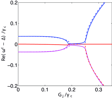
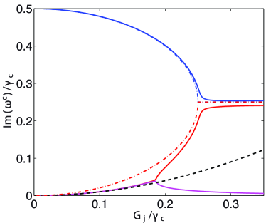
Figure 8: Comparison between the calculated values of $\omega_{1,2}^{c}$ with the values obtained by diagonalization of the equations of motion (solid lines). (Left:) Real part of the frequency. Dashed line is the weak-coupling expression obtained from Eq. (22) by using Eq. (24) and the dash-dotted line is obtained from the strong coupling expression Eq. (28). (Right): Effective linewidths of the modes. Black dashed line is from eqs. (23), showing the regular optically induced damping, whereas the dash-dotted lines are obtained from Eq. (28). These frequencies have been calculated with the same parameters as in the previous figures.

.

In Fig.8, we have compared the relevant eigenfrequencies around $-\Delta$ as obtained by the diagonalization of Eqs. (33) with the strong and weak coupling expansion for $\omega_{1\pm}^{c}$ and $\omega_{2}^{c}$. In the weak-coupling regime the eigenstates correspond (in the limit $G_{1,2}\to 0$) to the normal modes of the uncoupled system (i.e. cavity, mechanical resonator 1, mechanical resonator 2, cavity field). The corresponding eigenfrequencies match the expression given in Eq. (22) in the case where $\tilde{\chi}$ is independent of $\omega$.

In the strong-coupling regime these modes correspond to the coherent superposition of the cavity field and $q_{s\pm}$ modes or zero cavity field and $q_{a}$ modes. We can gain further insight about these modes by writing the strong-coupling version ($\omega_{\Delta}\ll G$) of the equation of motion (33c) in the sideband-resolved regime

$$\dot{a}_{a}=-i\omega_{\Sigma}a_{a}-\frac{\gamma}{2}a_{a}$$ (41)

$$\dot{a}_{s}=-i\omega_{\Sigma}a_{s}-\frac{\gamma}{2}a_{s}+\frac{iG}{\sqrt{2}}a$$ (42)

$$\dot{a}=i\Delta a+i\sqrt{2}Ga_{s}-\frac{\gamma_{c}}{2}a.$$ (43)

Its eigenfrequencies are given by

$$\omega_{A}=\omega_{\Sigma}$$ (44)

$$\omega_{B\pm}=-\Delta\pm 1/4\sqrt{16G^{2}-\gamma_{c}^{2}}.$$ (45)

Moreover, the eigenvector associated to $\omega_{A}$, corresponds (asymptotically) to a vector for which $a$ and $a_{s}$ are zero, while the eigenvectors associated to $\omega_{B\pm}$ correspond to vectors for which $a_{a}$ is zero, allowing thus to identify $\omega_{A}$ with the frequency of the dark mode and $\omega_{B\pm}$ to that of the bright modes.

The coupling $G=\gamma_{c}/4$ corresponds to the onset of the strong-coupling regime where, asymptotically, the eigenmodes correspond to the dark and bright modes. Moreover the limit $G\gg\gamma_{c}$ yields

$$\omega_{B\pm}=-\Delta\pm G,$$ (46)

allowing us to identify the symmetric mode $q_{s}$ with the mechanical component of the bright mode, as it can be seen from the expression giving the strong-coupling expansion of $\omega_{1}^{c}$ (see eqs. (22)).

References

- (1) Andre, A. et al. A coherent all-electrical interface between polar molecules and mesoscopic superconducting resonators. Nature Physics 2, 636–642 (2006).
- (2) Rosenberg, J., Lin, Q. & Painter, O. Static and dynamic wavelength routing via the gradient optical force. Nature Photonics 3, 478–483 (2009).
- (3) Zhu, X. et al. Coherent coupling of a superconducting flux qubit to an electron spin ensemble in diamond. Nature 478, 221–224 (2011).
- (4) Camerer, S. et al. Realization of an optomechanical interface between ultracold atoms and a membrane. Phys. Rev. Lett. 107, 223001 (2011).
- (5) O’Connell, A. D. et al. Quantum ground state and single-phonon control of a mechanical resonator. Nature 464, 697–703 (2010).
- (6) Kippenberg, T. J. & Vahala, K. J. Cavity optomechanics: Back-action at the mesoscale. Science 321, 1172–1176 (2008).
- (7) Metzger, C. H. & Karrai, K. Cavity cooling of a microlever. Nature 432, 1002–1005 (2004).
- (8) Rocheleau, T. et al. Preparation and detection of a mechanical resonator near the ground state of motion. Nature 463, 72–75 (2010).
- (9) Teufel, J. D. et al. Sideband cooling of micromechanical motion to the quantum ground state. Nature 475, 359–363 (2011).
- (10) Chan, J. et al. Laser cooling of a nanomechanical oscillator into its quantum ground state. Nature 478, 89–92 (2011).
- (11) Gröblacher, S., Hammerer, K., Vanner, M. R. & Aspelmeyer, M. Observation of strong coupling between a micromechanical resonator and an optical cavity field. Nature 460, 724–727 (2009).
- (12) LaHaye, M. D., Suh, J., Echternach, P. M., Schwab, K. C. & Roukes, M. L. Nanomechanical measurements of a superconducting qubit. Nature 459, 960–964 (2009).
- (13) Leggett, A. J. Testing the limits of quantum mechanics: motivation, state of play, prospects. Journal of Physics: Condensed Matter 14, R415 (2002).
- (14) Ansmann, M. et al. Violation of Bell’s inequality in Josephson phase qubits. Nature 461, 504–506 (2009).
- (15) Dobrindt, J. M. & Kippenberg, T. J. Theoretical analysis of mechanical displacement measurement using a multiple cavity mode transducer. Phys. Rev. Lett. 104, 033901 (2010).
- (16) Heinrich, G. & Marquardt, F. Coupled multimode optomechanics in the microwave regime. Europhysics Letters 93, 18003 (2011).
- (17) Lin, Q. et al. Coherent mixing of mechanical excitations in nano-optomechanical structures. Nature Photonics 4, 236–242 (2010).
- (18) Sulkko, J. et al. Strong Gate Coupling of High-Q Nanomechanical Resonators. Nano Lett. 10, 4884–4889 (2010).
- (19) Massel, F. et al. Microwave amplification with nanomechanical resonators. Nature 480, 351–354 (2011).
- (20) Faust, T., Krenn, P., Manus, S., Kotthaus, J. P. & Weig, E. M. Microwave cavity-enhanced transduction for plug and play nanomechanics at room temperature. Nature Communications 3, 728 (2012).
- (21) Teufel, J. D. et al. Circuit cavity electromechanics in the strong-coupling regime. Nature 471, 204–208 (2011).
- (22) Altomare, F. et al. Tripartite interactions between two phase qubits and a resonant cavity. Nature Physics 6, 777–781 (2010).
- (23) Fleischhauer, M., Imamoglu, A. & Marangos, J. P. Electromagnetically induced transparency: Optics in coherent media. Rev. Mod. Phys. 77, 633–673 (2005).
- (24) Regal, C. A., Teufel, J. D. & Lehnert, K. W. Measuring nanomechanical motion with a microwave cavity interferometer. Nature Physics 4, 555–560 (2008).
- (25) Schliesser, A., Arcizet, O., Riviere, R., Anetsberger, G. & Kippenberg, T. J. Resolved-sideband cooling and position measurement of a micromechanical oscillator close to the Heisenberg uncertainty limit. Nature Physics 5, 509–514 (2009).
- (26) Hertzberg, J. B. et al. Back-action-evading measurements of nanomechanical motion. Nature Physics 6, 213–217 (2010).
- (27) Mancini, S., Giovannetti, V., Vitali, D. & Tombesi, P. Entangling macroscopic oscillators exploiting radiation pressure. Phys. Rev. Lett. 88, 120401 (2002).
- (28) Vitali, D. et al. Optomechanical entanglement between a movable mirror and a cavity field. Phys. Rev. Lett. 98, 030405 (2007).
- (29) The LIGO Scientific Collaboration. A gravitational wave observatory operating beyond the quantum shot-noise limit. Nature Physics 7, 962–965 (2011).
- (30) Safavi-Naeini, A. H. et al. Electromagnetically induced transparency and slow light with optomechanics. Nature 472, 69–73 (2011).
- (31) Massel, F. et al. Microwave amplification with nanomechanical resonators: Supplementary information. Nature 480, 351–354 (2011).