Efficient Bayes-Adaptive Reinforcement Learning using Sample-Based Search

Abstract

Bayesian model-based reinforcement learning is a formally elegant approach to learning optimal behaviour under model uncertainty, trading off exploration and exploitation in an ideal way. Unfortunately, finding the resulting Bayes-optimal policies is notoriously taxing, since the search space becomes enormous. In this paper we introduce a tractable, sample-based method for approximate Bayes-optimal planning which exploits Monte-Carlo tree search. Our approach outperformed prior Bayesian model-based RL algorithms by a significant margin on several well-known benchmark problems – because it avoids expensive applications of Bayes rule within the search tree by lazily sampling models from the current beliefs. We illustrate the advantages of our approach by showing it working in an infinite state space domain which is qualitatively out of reach of almost all previous work in Bayesian exploration.

1 Introduction

A key objective in the theory of Markov Decision Processes (MDPs) is to maximize the expected sum of discounted rewards when the dynamics of the MDP are (perhaps partially) unknown. The discount factor pressures the agent to favor short-term rewards, but potentially costly exploration may identify better rewards in the long-term. This conflict leads to the well-known exploration-exploitation trade-off. One way to solve this dilemma [3, 10] is to augment the regular state of the agent with the information it has acquired about the dynamics. One formulation of this idea is the augmented Bayes-Adaptive MDP (BAMDP) [19, 9], in which the extra information is the posterior belief distribution over the dynamics, given the data so far observed. The agent starts in the belief state corresponding to its prior and, by executing the greedy policy in the BAMDP whilst updating its posterior, acts optimally (with respect to its beliefs) in the original MDP. In this framework, rich prior knowledge about statistics of the environment can be naturally incorporated into the planning process, potentially leading to more efficient exploration and exploitation of the uncertain world.

Unfortunately, exact Bayesian reinforcement learning is computationally intractable. Various algorithms have been devised to approximate optimal learning, but often at rather large cost. Here, we present a tractable approach that exploits and extends recent advances in Monte-Carlo tree search (MCTS) [17, 21], but avoiding problems associated with applying MCTS directly to the BAMDP.

At each iteration in our algorithm, a single MDP is sampled from the agent’s current beliefs. This MDP is used to simulate a single episode whose outcome is used to update the value of each node of the search tree traversed during the simulation. By integrating over many simulations, and therefore many sample MDPs, the optimal value of each future sequence is obtained with respect to the agent’s beliefs. We prove that this process converges to the Bayes-optimal policy, given infinite samples. To increase computational efficiency, we introduce a further innovation: a lazy sampling scheme that considerably reduces the cost of sampling.

We applied our algorithm to a representative sample of benchmark problems and competitive algorithms from the literature. It consistently and significantly outperformed existing Bayesian RL methods, and also recent non-Bayesian approaches, thus achieving state-of-the-art performance.

Our algorithm is more efficient than previous sparse sampling methods for Bayes-adaptive planning [26, 6, 2], partly because it does not update the posterior belief state during the course of each simulation. It thus avoids repeated applications of Bayes rule, which is expensive for all but the simplest priors over the MDP. Consequently, our algorithm is particularly well suited to support planning in domains with richly structured prior knowledge — a critical requirement for applications of Bayesian reinforcement learning to large problems. We illustrate this benefit by showing that our algorithm can tackle a domain with an infinite number of states and a structured prior over the dynamics, a challenging — if not intractable — task for existing approaches.

2 Bayesian RL

We describe the generic Bayesian formulation of optimal decision-making in an unknown MDP, following [19] and [9]. An MDP is described as a 5-tuple $M=\langle S,A,\mathcal{P},\mathcal{R},\gamma\rangle$, where $S$ is the set of states, $A$ is the set of actions, $\mathcal{P}:S\times A\times S\rightarrow\mathbb{R}$ is the state transition probability kernel, $\mathcal{R}:S\times A\rightarrow\mathbb{R}$ is a bounded reward function, and $\gamma$ is the discount factor [24]. When all the components of the MDP tuple are known, standard MDP planning algorithms can be used to estimate the optimal value function and policy off-line. In general, the dynamics are unknown, and we assume that $\mathcal{P}$ is a latent variable distributed according to a distribution $P(\mathcal{P})$. After observing a history of actions and states $h_{t}=s_{1}a_{1}s_{2}a_{2}\dots a_{t-1}s_{t}$ from the MDP, the posterior belief on $\mathcal{P}$ is updated using Bayes’ rule $P(\mathcal{P}|h_{t})\propto P(h_{t}|\mathcal{P})P(\mathcal{P})$. The uncertainty about the dynamics of the model can be transformed into uncertainty about the current state inside an augmented state space $S^{+}=S\times\mathcal{H}$, where $S$ is the state space in the original problem and $\mathcal{H}$ is the set of possible histories. The dynamics associated with this augmented state space are described by

$$\mathcal{P}^{+}(\langle s,h\rangle,a,\langle s^{\prime},h^{\prime}\rangle)=\mathds{1}[h^{\prime}=has^{\prime}]\int_{\mathcal{P}}\mathcal{P}(s,a,s^{\prime})P(\mathcal{P}|h)\,\text{d}\mathcal{P},\;\;\;\;\mathcal{R}^{+}(\langle s,h\rangle,a)=R(s,a)$$ (1)

Together, the 5-tuple $M^{+}=\langle S^{+},A,\mathcal{P}^{+},\mathcal{R}^{+},\gamma\rangle$ forms the Bayes-Adaptive MDP (BAMDP) for the MDP problem $M$. Since the dynamics of the BAMDP are known, it can in principle be solved to obtain the optimal value function associated with each action:

$$Q^{*}(\langle s_{t},h_{t}\rangle,a)=\max_{\pi}\mathbb{E}_{\pi}\left[\sum_{t^{\prime}=t}^{\infty}\gamma^{t^{\prime}-t}r_{t^{\prime}}|a_{t}=a\right]$$ (2)

from which the optimal action for each state can be readily derived.  Optimal actions in the BAMDP are executed greedily in the real MDP $M$ and constitute the best course of action for a Bayesian agent with respect to its prior belief over $\mathcal{P}$. It is obvious that the expected performance of the BAMDP policy in the MDP $M$ is bounded above by that of the optimal policy obtained with a fully-observable model, with equality occurring, for example, in the degenerate case in which the prior only has support on the true model.

3 The BAMCP algorithm

3.1 Algorithm Description

The goal of a BAMDP planning method is to find, for each decision point $\langle s,h\rangle$ encountered, the action $a$ that maximizes Equation 2. Our algorithm, Bayes-adaptive Monte-Carlo Planning (BAMCP), does this by performing a forward-search in the space of possible future histories of the BAMDP using a tailored Monte-Carlo tree search.

We employ the UCT algorithm [17] to allocate search effort to promising branches of the state-action tree, and use sample-based rollouts to provide value estimates at each node. For clarity, let us denote by Bayes-Adaptive UCT (BA-UCT) the algorithm that applies vanilla UCT to the BAMDP (i.e., the particular MDP with dynamics described in Equation 1). Sample-based search in the BAMDP using BA-UCT requires the generation of samples from $\mathcal{P}^{+}$ at every single node. This operation requires integration over all possible transition models, or at least a sample of a transition model $\mathcal{P}$ — an expensive procedure for all but the simplest generative models $P(\mathcal{P})$. We avoid this cost by only sampling a single transition model $\mathcal{P}^{i}$ from the posterior at the root of the search tree at the start of each simulation $i$, and using $\mathcal{P}^{i}$ to generate all the necessary samples during this simulation. Sample-based tree search then acts as a filter, ensuring that the correct distribution of state successors is obtained at each of the tree nodes, as if it was sampled from $\mathcal{P}^{+}$. This root sampling method was originally introduced in the POMCP algorithm [21], developed to solve Partially Observable MDPs.

3.2 BA-UCT with Root Sampling

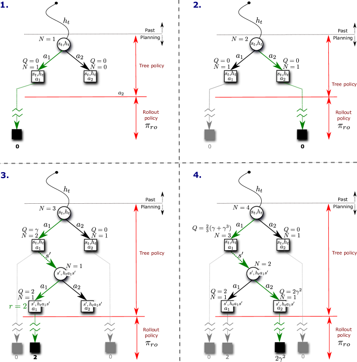
Figure S3: This diagram presents the first 4 simulations of BAMCP in an MDP with 2 actions from state $\langle s_{t},h_{t}\rangle$. The rollout trajectories are represented with dotted lines (green for the current rollouts, and greyed out for past rollouts). 1. The root node is expanded with two action nodes. Action $a_{1}$ is chosen at the root (random tie-breaking) and a rollout is executed in $\mathcal{P}^{1}$ with a resulting value estimate of 0. Counts $N(\langle s_{t},h_{t}\rangle)$ and $N(\langle s_{t},h_{t}\rangle,a_{1})$, and value $Q(\langle s_{t},h_{t}\rangle,a_{1})$ get updated. 2. Action $a_{2}$ is chosen at the root and a rollout is executed with value estimate 0. Counts and value get updated. 3. Action $a_{1}$ is chosen (tie-breaking), then $s^{\prime}$ is sampled from $\mathcal{P}^{3}(s_{t},a_{1},\cdot)$. State node $\langle s^{\prime},h_{t}a_{1}s^{\prime}\rangle$ gets expanded and action $a_{1}$ is selected, incurring a reward of $2$, followed by a rollout. 4. The UCB rule selects action $a_{1}$ at the top, the successor state $s^{\prime}$ is sampled from $\mathcal{P}^{4}(s_{t},a_{1},\cdot)$. Action $a_{2}$ is chosen from the internal node $\langle s^{\prime},h_{t}a_{1}s^{\prime}\rangle$, followed by a rollout using $\mathcal{P}^{4}$ and $\pi_{ro}$. A reward of $2$ is obtained after $2$ steps from that tree node. Counts for the traversed nodes are updated and the MC backup updates $Q(\langle s^{\prime},h_{t}a_{1}s^{\prime}\rangle,a_{1})$ to $R=0+\gamma 0+\gamma^{2}2+\gamma^{3}0+\dots=\gamma^{2}2$ and $Q(\langle s_{t},h_{t}\rangle,a_{1})$ to $\gamma+\nicefrac{{2\gamma^{3}-\gamma}}{{3}}=\frac{2}{3}(\gamma+\gamma^{3})$.

The root node of the search tree at a decision point represents the current state of the BAMDP. The tree is composed of state nodes representing belief states $\langle s,h\rangle$ and action nodes representing the effect of particular actions from their parent state node. The visit counts: $N(\langle s,h\rangle)$ for state nodes, and $N(\langle s,h\rangle,a)$ for action nodes, are initialized to $0$ and updated throughout search. A value $Q(\langle s,h\rangle,a)$, initialized to $0$, is also maintained for each action node. Each simulation traverses the tree without backtracking by following the UCT policy at state nodes defined by $\operatornamewithlimits{argmax}_{a}Q(\langle s,h\rangle,a)+c\sqrt{\nicefrac{{\log(N(\langle s,h\rangle))}}{{N(\langle s,h\rangle,a)}}}$, where $c$ is an exploration constant that needs to be set appropriately. Given an action, the transition distribution $\mathcal{P}^{i}$ corresponding to the current simulation $i$ is used to sample the next state. That is, at action node $(\langle s,h\rangle,a)$, $s^{\prime}$ is sampled from $\mathcal{P}^{i}(s,a,\cdot)$, and the new state node is set to $\langle s^{\prime},has^{\prime}\rangle$. When a simulation reaches a leaf, the tree is expanded by attaching a new state node with its connected action nodes, and a rollout policy $\pi_{ro}$ is used to control the MDP defined by the current $\mathcal{P}^{i}$ to some fixed depth (determined using the discount factor). The rollout provides an estimate of the value $Q(\langle s,h\rangle,a)$ from the leaf action node. This estimate is then used to update the value of all action nodes traversed during the simulation: if $R$ is the sampled discounted return obtained from a traversed action node ($\langle s,h\rangle,a$) in a given simulation, then we update the value of the action node to $Q(\langle s,h\rangle,a)+\nicefrac{{R-Q(\langle s,h\rangle,a)}}{{N(\langle s,h\rangle,a)}}$ (i.e., the mean of the sampled returns obtained from that action node over the simulations). A detailed description of the BAMCP algorithm is provided in Algorithm 1. A diagram example of BAMCP simulations is presented in Figure S3.

The tree policy treats the forward search as a meta-exploration problem, preferring to exploit regions of the tree that currently appear better than others while continuing to explore unknown or less known parts of the tree. This leads to good empirical results even for small number of simulations, because effort is expended where search seems fruitful. Nevertheless all parts of the tree are eventually visited infinitely often, and therefore the algorithm will eventually converge on the Bayes-optimal policy (see Section 3.5).

procedure Search( $\langle s,h\rangle$ )

repeat

      $\mathcal{P}\sim P(\mathcal{P}|h)$

      Simulate($\langle s,h\rangle,\mathcal{P},0$)

      until Timeout()

     return $\displaystyle\operatornamewithlimits{argmax}_{a}\;Q(\langle s,h\rangle,a)$

      end procedure

     

     

      procedure Rollout(​​​ $\langle s,h\rangle,\mathcal{P},d$ )

      if $\gamma^{d}Rmax<\epsilon$ then

           return $0$

          

           end $a\sim\pi_{ro}(\langle s,h\rangle,\cdot)$

           $s^{\prime}\sim\mathcal{P}(s,a,\cdot)$

           $r\leftarrow\mathcal{R}(s,a)$

           return $r\!+\!\gamma$Rollout($\langle s^{\prime},has^{\prime}\rangle,\mathcal{P},d\!+\!1$)

           end procedure

          

          

          

Algorithm 1 BAMCP

procedure Simulate( $\langle s,h\rangle,\mathcal{P},d$)

if $\gamma^{d}Rmax<\epsilon$ then return $0$

if $N(\langle s,h\rangle)=0$ then

      for all $a\in A$ do

           $N(\langle s,h\rangle,a)\leftarrow 0$, $Q(\langle s,h\rangle,a))\leftarrow 0$

          

           end $a\sim\pi_{ro}(\langle s,h\rangle,\cdot)$

           $s^{\prime}\sim\mathcal{P}(s,a,\cdot)$

           $r\leftarrow\mathcal{R}(s,a)$

           $R\leftarrow r+\gamma$ Rollout($\langle s^{\prime},has^{\prime}\rangle,\mathcal{P},d$)

           $N(\langle s,h\rangle)\leftarrow 1$, $N(\langle s,h\rangle,a)\leftarrow 1$

           $Q(\langle s,h\rangle,a)\leftarrow R$

           return $R$

          

           end $a\leftarrow\displaystyle\operatornamewithlimits{argmax}_{b}Q(\langle s,h\rangle,b)+c\sqrt{\tfrac{\log(N(\langle s,h\rangle))}{N(\langle s,h\rangle,b)}}$

           $s^{\prime}\sim\mathcal{P}(s,a,\cdot)$

           $r\leftarrow\mathcal{R}(s,a)$

           $R\leftarrow r+\gamma$ Simulate($\langle s^{\prime},has^{\prime}\rangle,\mathcal{P},d\!+\!1$)

           $N(\langle s,h\rangle)\leftarrow N(\langle s,h\rangle)+1$

           $N(\langle s,h\rangle,a)\leftarrow N(\langle s,h\rangle,a)+1$

           $Q(\langle s,h\rangle,a)\leftarrow Q(\langle s,h\rangle,a)+\frac{R-Q(\langle s,h\rangle,a)}{N(\langle s,h\rangle,a)}$

           return $R$

           end procedure

Finally, note that the history of transitions $h$ is generally not the most compact sufficient statistic of the belief in fully observable MDPs. Indeed, it can be replaced with unordered transition counts $\psi$, considerably reducing the number of states of the BAMDP and, potentially the complexity of planning. Given an addressing scheme suitable to the resulting expanding lattice (rather than to a tree), BAMCP can search in this reduced space. We found this version of BAMCP to offer only a marginal improvement. This is a common finding for UCT, stemming from its tendency to concentrate search effort on one of several equivalent paths (up to transposition), implying a limited effect on performance of reducing the number of those paths.

3.3 Lazy Sampling

In previous work on sample-based tree search, indeed including POMCP [21], a complete sample state is drawn from the posterior at the root of the search tree. However, this can be computationally very costly. Instead, we sample $\mathcal{P}$ lazily, creating only the particular transition probabilities that are required as the simulation traverses the tree, and also during the rollout.

Consider $\mathcal{P}(s,a,\cdot)$ to be parametrized by a latent variable $\theta_{s,a}$ for each state and action pair. These may depend on each other, as well as on an additional set of latent variables $\phi$. The posterior over $\mathcal{P}$ can be written as $P(\Theta|h)=\int_{\phi}P(\Theta|\phi,h)P(\phi|h)$, where $\Theta=\{\theta_{s,a}|s\in S,a\in A\}$. Define $\Theta_{t}=\{\theta_{s_{1},a_{1}},\cdots,\theta_{s_{t},a_{t}}\}$ as the (random) set of $\theta$ parameters required during the course of a BAMCP simulation that starts at time $1$ and ends at time $t$. Using the chain rule, we can rewrite

$$P(\Theta|\phi,h)=P(\theta_{s_{1},a_{1}}|\phi,h)P(\theta_{s_{2},a_{2}}|\Theta_{1},\phi,h)\dots P(\theta_{s_{T},a_{T}}|\Theta_{T-1},\phi,h)P(\Theta\setminus\Theta_{T}|\Theta_{T},\phi,h)$$

where $T$ is the length of the simulation and $\Theta\setminus\Theta_{T}$ denotes the (random) set of parameters that are not required for a simulation. For each simulation $i$, we sample $P(\phi|h_{t})$ at the root and then lazily sample the $\theta_{s_{t},a_{t}}$ parameters as required, conditioned on $\phi$ and all $\Theta_{t-1}$ parameters sampled for the current simulation. This process is stopped at the end of the simulation, potentially before all $\theta$ parameters have been sampled. For example, if the transition parameters for different states and actions are independent, we can completely forgo sampling a complete $\mathcal{P}$, and instead draw any necessary parameters individually for each state-action pair. This leads to substantial performance improvement, especially in large MDPs where a single simulation only requires a small subset of parameters (see for example the domain in Section 5.2).

3.4 Rollout Policy Learning

The choice of rollout policy $\pi_{ro}$ is important if simulations are few, especially if the domain does not display substantial locality or if rewards require a carefully selected sequence of actions to be obtained. Otherwise, a simple uniform random policy can be chosen to provide noisy estimates. In this work, we learn $Q_{ro}$, the optimal $Q$-value in the real MDP, in a model-free manner (e.g., using Q-learning) from samples $(s_{t},a_{t},r_{t},s_{t+1})$ obtained off-policy as a result of the interaction of the Bayesian agent with the environment. Acting greedily according to $Q_{ro}$ translates to pure exploitation of gathered knowledge. A rollout policy in BAMCP following $Q_{ro}$ could therefore over-exploit. Instead, similar to [13], we select an $\epsilon$-greedy policy with respect to $Q_{ro}$ as our rollout policy $\pi_{ro}$. This biases rollouts towards observed regions of high rewards. This method provides valuable direction for the rollout policy at negligible computational cost. More complex rollout policies can be considered, for example rollout policies that depend on the sampled model $\mathcal{P}^{i}$. However, these usually incur computational overhead.

3.5 Theoretical properties

Define $V(\langle s,h\rangle)=\displaystyle\max_{a\in A}Q(\langle s,h\rangle,a)\;\;\forall\langle s,h\rangle\in S\times\mathcal{H}$.

Theorem 1.

For all $\epsilon>0$ (the numerical precision, see Algorithm 1) and a suitably chosen $c$ (e.g. $c>\frac{Rmax}{1-\gamma}$), from state $\langle s_{t},h_{t}\rangle$, BAMCP constructs a value function at the root node that converges in probability to an $\epsilon^{\prime}$-optimal value function, $V(\langle s_{t},h_{t}\rangle)\overset{p}{\rightarrow}V^{*}_{\epsilon^{\prime}}(\langle s_{t},h_{t}\rangle)$, where $\epsilon^{\prime}=\frac{\epsilon}{1-\gamma}$. Moreover, for large enough $N(\langle s_{t},h_{t}\rangle)$, the bias of $V(\langle s_{t},h_{t}\rangle)$ decreases as $O(\log(N(\langle s_{t},h_{t}\rangle))/N(\langle s_{t},h_{t}\rangle))$. (Proof available in supplementary material)

By definition, Theorem 1 implies that BAMCP converges to the Bayes-optimal solution asymptotically. We confirmed this result empirically using a variety of Bandit problems, for which the Bayes-optimal solution can be computed efficiently using Gittins indices (see supplementary material).

4 Related Work

In Section 5, we compare BAMCP to a set of existing Bayesian RL algorithms. Given limited space, we do not provide a comprehensive list of planning algorithms for MDP exploration, but rather concentrate on related sample-based algorithms for Bayesian RL.

Bayesian DP [23] maintains a posterior distribution over transition models. At each step, a single model is sampled, and the action that is optimal in that model is executed. The Best Of Sampled Set (BOSS) algorithm generalizes this idea [1]. BOSS samples a number of models from the posterior and combines them optimistically. This drives sufficient exploration to guarantee finite-sample performance guarantees. BOSS is quite sensitive to its parameter that governs the sampling criterion. Unfortunately, this is difficult to select. Castro and Precup proposed an SBOSS variant, which provides a more effective adaptive sampling criterion [5]. BOSS algorithms are generally quite robust, but suffer from over-exploration.

Sparse sampling [16] is a sample-based tree search algorithm. The key idea is to sample successor nodes from each state, and apply a Bellman backup to update the value of the parent node from the values of the child nodes. Wang et al. applied sparse sampling to search over belief-state MDPs[26]. The tree is expanded non-uniformly according to the sampled trajectories. At each decision node, a promising action is selected using Thompson sampling — i.e., sampling an MDP from that belief-state, solving the MDP and taking the optimal action. At each chance node, a successor belief-state is sampled from the transition dynamics of the belief-state MDP.

Asmuth and Littman further extended this idea in their BFS3 algorithm [2], an adaptation of Forward Search Sparse Sampling [25] to belief-MDPs. Although they described their algorithm as Monte-Carlo tree search, it in fact uses a Bellman backup rather than Monte-Carlo evaluation. Each Bellman backup updates both lower and upper bounds on the value of each node. Like Wang et al., the tree is expanded non-uniformly according to the sampled trajectories, albeit using a different method for action selection. At each decision node, a promising action is selected by maximising the upper bound on value. At each chance node, observations are selected by maximising the uncertainty (upper minus lower bound).

Bayesian Exploration Bonus (BEB) solves the posterior mean MDP, but with an additional reward bonus that depends on visitation counts [18]. Similarly, Sorg et al. propose an algorithm with a different form of exploration bonus [22]. These algorithms provide performance guarantees after a polynomial number of steps in the environment. However, behavior in the early steps of exploration is very sensitive to the precise exploration bonuses; and it turns out to be hard to translate sophisticated prior knowledge into the form of a bonus.

Table 1: Experiment results summary. For each algorithm, we report the mean sum of rewards and confidence interval for the best performing parameter within a reasonable planning time limit (0.25 s/step for Double-loop, 1 s/step for Grid5 and Grid10, 1.5 s/step for the Maze). For BAMCP, this simply corresponds to the number of simulations that achieve a planning time just under the imposed limit. * Results reported from [23] without timing information.

	Double-loop	Grid5	Grid10	Dearden’s Maze
BAMCP	387.6 $\pm$ 1.5	72.9 $\pm$ 3	32.7 $\pm$ 3	965.2 $\pm$ 73
BFS3 [2]	382.2 $\pm$ 1.5	66 $\pm$ 5	10.4 $\pm$ 2	240.9 $\pm$ 46
SBOSS [5]	371.5 $\pm$ 3	59.3 $\pm$ 4	21.8 $\pm$ 2	671.3 $\pm$ 126
BEB [18]	386 $\pm$ 0	67.5 $\pm$ 3	10 $\pm$ 1	184.6 $\pm$ 35
Bayesian DP* [23]	377 $\pm$ 1	-	-	-
Bayes VPI+MIX* [8]	326 $\pm$ 31	-	-	817.6 $\pm$ 29
IEQL+* [20]	264 $\pm$ 1	-	-	269.4 $\pm$ 1
QL Boltzmann*	186 $\pm$ 1	-	-	195.2 $\pm$ 20

5 Experiments

We first present empirical results of BAMCP on a set of standard problems with comparisons to other popular algorithms. Then we showcase BAMCP’s advantages in a large scale task: an infinite 2D grid with complex correlations between reward locations.

5.1 Standard Domains

Algorithms

The following algorithms were run: BAMCP - The algorithm presented in Section 3, implemented with lazy sampling. The algorithm was run for different number of simulations (10 to 10000) to span different planning times. In all experiments, we set $\pi_{\text{ro}}$ to be an $\epsilon$-greedy policy with $\epsilon=0.5$. The UCT exploration constant was left unchanged for all experiments $(c=3)$, we experimented with other values of $c\in\{0.5,1,5\}$ with similar results. SBOSS [5]: for each domain, we varied the number of samples $K\in\{2,4,8,16,32\}$ and the resampling threshold parameter $\delta\in\{3,5,7\}$. BEB [18]: for each domain, we varied the bonus parameter $\beta\in\{0.5,1,1.5,2,2.5,3,5,10,15,20\}$. BFS3 [2] for each domain, we varied the branching factor $C\in\{2,5,10,15\}$ and the number of simulations (10 to 2000). The depth of search was set to $15$ in all domains except for the larger grid and maze domain where it was set to $50$. We also tuned the $V_{\text{max}}$ parameter for each domain — $V_{\text{min}}$ was always set to $0$. In addition, we report results from [23] for several other prior algorithms.

Domains

For all domains, we fix $\gamma=0.95$. The Double-loop domain is a $9$-state deterministic MDP with $2$ actions [8], $1000$ steps are executed in this domain. Grid5 is a $5\times 5$ grid with no reward anywhere except for a reward state opposite to the reset state. Actions with cardinal directions are executed with small probability of failure for $1000$ steps. Grid10 is a $10\times 10$ grid designed like Grid5. We collect $2000$ steps in this domain. Dearden’s Maze is a $264$-states maze with $3$ flags to collect [8]. A special reward state gives the number of flags collected since the last visit as reward, $20000$ steps are executed in this domain. 

To quantify the performance of each algorithm, we measured the total undiscounted reward over many steps. We chose this measure of performance to enable fair comparisons to be drawn with prior work. In fact, we are optimising a different criterion – the discounted reward from the start state – and so we might expect this evaluation to be unfavourable to our algorithm.

One major advantage of Bayesian RL is that one can specify priors about the dynamics. For the Double-loop domain, the Bayesian RL algorithms were run with a simple Dirichlet-Multinomial model with symmetric Dirichlet parameter $\alpha=\frac{1}{|S|}$. For the grids and the maze domain, the algorithms were run with a sparse Dirichlet-Multinomial model, as described in [11]. For both of these models, efficient collapsed sampling schemes are available; they are employed for the BA-UCT and BFS3 algorithms in our experiments to compress the posterior parameter sampling and the transition sampling into a single transition sampling step. This considerably reduces the cost of belief updates inside the search tree when using these simple probabilistic models. In general, efficient collapsed sampling schemes are not available (see for example the model in Section 5.2).

(a)

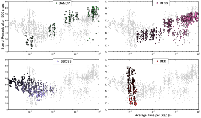
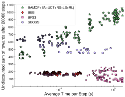
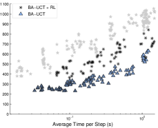
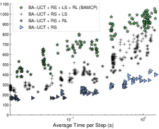
Figure 1: Performance of each algorithm on the Grid5 (a.) and Maze domain (b-d) as a function of planning time. Each point corresponds to a single run of an algorithm with an associated setting of the parameters. Increasing brightness inside the points codes for an increasing value of a parameter (BAMCP and BFS3: number of simulations, BEB: bonus parameter $\beta$, SBOSS: number of samples $K$). A second dimension of variation is coded as the size of the points (BFS3: branching factor $C$, SBOSS: resampling parameter $\delta$). The range of parameters is specified in Section 5.1. a. Performance of each algorithm on the Grid5 domain. b. Performance of each algorithm on the Maze domain. c. On the Maze domain, performance of vanilla BA-UCT with and without rollout policy learning (RL). d. On the Maze domain, performance of BAMCP with and without the lazy sampling (LS) and rollout policy learning (RL) presented in Sections 3.4, 3.3. Root sampling (RS) is included.

Results

A summary of the results is presented in Table 1. Figure 1 reports the planning time/performance trade-off for the different algorithms on the Grid5 and Maze domain.

On all the domains tested, BAMCP performed best. Other algorithms came close on some tasks, but only when their parameters were tuned to that specific domain. This is particularly evident for BEB, which required a different value of exploration bonus to achieve maximum performance in each domain. BAMCP’s performance is stable with respect to the choice of its exploration constant $c$ and it did not require tuning to obtain the results.

BAMCP’s performance scales well as a function of planning time, as is evident in Figure 1. In contrast, SBOSS follows the opposite trend. If more samples are employed to build the merged model, SBOSS actually becomes too optimistic and over-explores, degrading its performance. BEB cannot take advantage of prolonged planning time at all. BFS3 generally scales up with more planning time with an appropriate choice of parameters, but it is not obvious how to trade-off the branching factor, depth, and number of simulations in each domain. BAMCP greatly benefited from our lazy sampling scheme in the experiments, providing $35\times$ speed improvement over the naive approach in the maze domain for example; this is illustrated in Figure 1.

Dearden’s maze aptly illustrates a major drawback of forward search sparse sampling algorithms such as BFS3. Like many maze problems, all rewards are zero for at least $k$ steps, where $k$ is the solution length. Without prior knowledge of the optimal solution length, all upper bounds will be higher than the true optimal value until the tree has been fully expanded up to depth $k$ – even if a simulation happens to solve the maze. In contrast, once BAMCP discovers a successful simulation, its Monte-Carlo evaluation will immediately bias the search tree towards the successful trajectory.

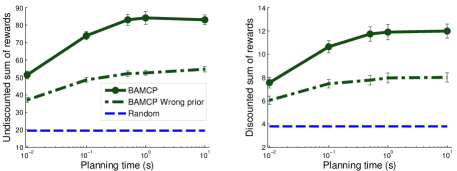
Figure 2: Performance of BAMCP as a function of planning time on the Infinite 2D grid task of Section 5.2, for $\gamma=0.97$, where the grids are generated with Beta parameters $\alpha_{1}=1,\beta_{1}=2,\alpha_{2}=2,\beta_{2}=1$ (See supp. Figure S4 for a visualization). The performance during the first 200 steps in the environment is averaged over 50 sampled environments (5 runs for each sample) and is reported both in terms of undiscounted (left) and discounted (right) sum of rewards. BAMCP is run either with the correct generative model as prior or with an incorrect prior (parameters for rows and columns are swapped), it is clear that BAMCP can take advantage of correct prior information to gain more rewards. The performance of a uniform random policy is also reported.

5.2 Infinite 2D grid task

We also applied BAMCP to a much larger problem. The generative model for this infinite-grid MDP is as follows: each column $i$ has an associated latent parameter $p_{i}\sim\text{Beta}(\alpha_{1},\beta_{1})$ and each row $j$ has an associated latent parameter $q_{j}\sim\text{Beta}(\alpha_{2},\beta_{2})$. The probability of grid cell $ij$ having a reward of $1$ is $p_{i}q_{j}$, otherwise the reward is $0$. The agent knows it is on a grid and is always free to move in any of the four cardinal directions. Rewards are consumed when visited; returning to the same location subsequently results in a reward of 0. As opposed to the independent Dirichlet priors employed in standard domains, here, dynamics are tightly correlated across states (i.e., observing a state transition provides information about other state transitions). Posterior inference (of the dynamics $\operatorname{\mathcal{P}}$) in this model requires approximation because of the non-conjugate coupling of the variables, the inference is done via MCMC (details in Supplementary). The domain is illustrated in Figure S4.

Planning algorithms that attempt to solve an MDP based on sample(s) (or the mean) of the posterior (e.g., BOSS, BEB, Bayesian DP) cannot directly handle the large state space. Prior forward-search methods (e.g., BA-UCT, BFS3) can deal with the state space, but not the large belief space: at every node of the search tree they must solve an approximate inference problem to estimate the posterior beliefs. In contrast, BAMCP limits the posterior inference to the root of the search tree and is not directly affected by the size of the state space or belief space, which allows the algorithm to perform well even with a limited planning time. Note that lazy sampling is required in this setup since a full sample of the dynamics involves infinitely many parameters.

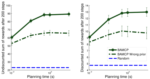
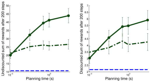
(b)

Figure S5: Performance of BAMCP on the Infinite 2D grid task of Section 5.2, for $\gamma=0.97$, as in Figure 2 but where the grids are generated with Beta parameters (a) $\alpha_{1}=0.5,\beta_{1}=0.5,\alpha_{2}=0.5,\beta_{2}=0.5$ and (b) $\alpha_{1}=0.5,\beta_{1}=0.5,\alpha_{2}=1,\beta_{2}=3$. In the wrong prior scenario (green dotted line), BAMCP is given the parameters (a) $\alpha_{1}=4,\beta_{1}=1,\alpha_{2}=0.5,\beta_{2}=0.5$ and (b) $\alpha_{1}=1,\beta_{1}=3,\alpha_{2}=0.5,\beta_{2}=0.5$. The behavior of the agent is qualitatively different depending on the prior parameters employed (see supplementary videos). For example, for the scenario in Figure 2, rewards are often found in relatively dense blocks on the map and the agents exploits this fact when exploring; for the scenario (b) of this Figure, good rewards rates can be obtained by following the rare rows that have high $q_{j}$ parameters, but finding good rows can be expensive so the agent might settle on sub-optimal rows (as in Bandit problems where the Bayes-optimal agent might settle on sub-optimal arm if it believes it likely is the best arm given past data). It should be pointed out that the actual Bayes-optimal strategy in this domain is not known — the behavior of BAMCP for finite planning time might not qualitatively match the Bayes-optimal strategy.

Figure 2 (and Figure S5) demonstrates the planning performance of BAMCP in this complex domain. Performance improves with additional planning time, and the quality of the prior clearly affects the agent’s performance. Supplementary videos contrast the behavior of the agent for different prior parameters.

6 Future Work

The UCT algorithm is known to have several drawbacks. First, there are no finite-time regret bounds. It is possible to construct malicious environments, for example in which the optimal policy is hidden in a generally low reward region of the tree, where UCT can be misled for long periods [7]. Second, the UCT algorithm treats every action node as a multi-armed bandit problem. However, there is no actual benefit to accruing reward during planning, and so it is in theory more appropriate to use pure exploration bandits [4]. Nevertheless, the UCT algorithm has produced excellent empirical performance in many domains [12].

BAMCP is able to exploit prior knowledge about the dynamics in a principled manner. In principle, it is possible to encode many aspects of domain knowledge into the prior distribution. An important avenue for future work is to explore rich, structured priors about the dynamics of the MDP. If this prior knowledge matches the class of environments that the agent will encounter, then exploration could be significantly accelerated.

7 Conclusion

We suggested a sample-based algorithm for Bayesian RL called BAMCP that significantly surpassed the performance of existing algorithms on several standard tasks. We showed that BAMCP can tackle larger and more complex tasks generated from a structured prior, where existing approaches scale poorly. In addition, BAMCP provably converges to the Bayes-optimal solution.

The main idea is to employ Monte-Carlo tree search to explore the augmented Bayes-adaptive search space efficiently. The naive implementation of that idea is the proposed BA-UCT algorithm, which cannot scale for most priors due to expensive belief updates inside the search tree. We introduced three modifications to obtain a computationally tractable sample-based algorithm: root sampling, which only requires beliefs to be sampled at the start of each simulation (as in [21]); a model-free RL algorithm that learns a rollout policy; and the use of a lazy sampling scheme to sample the posterior beliefs cheaply.

Supplementary Material

Proof of Theorem 1 and comments

Consider the BA-UCT algorithm: UCT applied to the Bayes-Adaptive MDP (dynamics are described in Equation 1). Let $\operatorname{\mathcal{D}}^{\pi}(h_{T})$ be the rollout distribution of BA-UCT: the probability that history $h_{T}$ is generated when running the BA-UCT search from $\langle s_{t},h_{t}\rangle$, with $h_{t}$ a prefix of $h_{T}$, $T-t$ the effective horizon in the search tree, and $\pi$ an arbitrary BAMDP policy. Similarly define the similar quantity $\tilde{\operatorname{\mathcal{D}}}^{\pi}(h_{T})$: the probability that history $h_{T}$ is generated when running the BAMCP algorithm. The following lemma shows that these two quantities are in fact equivalent.

Lemma 1.

$\operatorname{\mathcal{D}}^{\pi}(h_{T})=\tilde{\operatorname{\mathcal{D}}}^{\pi}(h_{T})$ for all BAMDP policies $\pi:\mathcal{H}\rightarrow A$.

Proof.

Let $\pi$ be arbitrary. We show by induction that for all suffix histories $h$ of $h_{t}$, $\operatorname{\mathcal{D}}^{\pi}(h)=\tilde{\operatorname{\mathcal{D}}}^{\pi}(h)$; but also $P(\operatorname{\mathcal{P}}|h)=\tilde{P}_{h}(\operatorname{\mathcal{P}})$ where $P(\operatorname{\mathcal{P}}|h)$ denotes (as before) the posterior distribution over the dynamics given $h$ and $\tilde{P}_{h}(\operatorname{\mathcal{P}})$ denotes the distribution of $\operatorname{\mathcal{P}}$ at node $h$ when running BAMCP.

Base case: At the root ($h=h_{t}$, suffix history of size 0), it is clear that $\tilde{P}_{h_{t}}(\operatorname{\mathcal{P}})=P(\operatorname{\mathcal{P}}|h_{t})$ since we are sampling from the posterior at the root node and $D^{\pi}(h_{t})=\tilde{\operatorname{\mathcal{D}}}^{\pi}(h_{t})=1$ since all simulations go through the root node.

Step case:

Assume proposition true for all suffices of size $i$. Consider any suffix $has^{\prime}$ of size $i+1$, where $a\in A$ and $s^{\prime}\in S$ are arbitrary and $h$ is an arbitrary suffix of size $i$ ending in $s$. The following relation holds:

$$\operatorname{\mathcal{D}}^{\pi}(has^{\prime}) =\operatorname{\mathcal{D}}^{\pi}(h)\pi(h,a)\int_{\operatorname{\mathcal{P}}}\mathrm{d}\!\operatorname{\mathcal{P}}P(\operatorname{\mathcal{P}}|h)\operatorname{\mathcal{P}}(s,a,s^{\prime})$$ (3)

$$=\tilde{\operatorname{\mathcal{D}}}^{\pi}(h)\pi(h,a)\int_{\operatorname{\mathcal{P}}}\mathrm{d}\!\operatorname{\mathcal{P}}\tilde{P}_{h}(\operatorname{\mathcal{P}})\operatorname{\mathcal{P}}(s,a,s^{\prime})$$ (4)

$$=\tilde{\operatorname{\mathcal{D}}}^{\pi}(has^{\prime}),$$ (5)

where the second line is obtained using the induction hypothesis, and the rest from the definitions. In addition, we can match the distribution of the samples $\operatorname{\mathcal{P}}$ at node $has^{\prime}$:

$$P(\operatorname{\mathcal{P}}|has^{\prime}) =P(has^{\prime}|\operatorname{\mathcal{P}})P(\operatorname{\mathcal{P}})/P(has^{\prime})$$ (6)

$$=P(h|\operatorname{\mathcal{P}})P(\operatorname{\mathcal{P}})\operatorname{\mathcal{P}}(s,a,s^{\prime})/P(has^{\prime})$$ (7)

$$=P(\operatorname{\mathcal{P}}|h)P(h)\operatorname{\mathcal{P}}(s,a,s^{\prime})/P(has^{\prime})$$ (8)

$$=ZP(\operatorname{\mathcal{P}}|h)\operatorname{\mathcal{P}}(s,a,s^{\prime})$$ (9)

$$=Z\tilde{P}_{h}(\operatorname{\mathcal{P}})\operatorname{\mathcal{P}}(s,a,s^{\prime})$$ (10)

$$=Z\tilde{P}_{ha}(\operatorname{\mathcal{P}})\operatorname{\mathcal{P}}(s,a,s^{\prime})$$ (11)

$$=\tilde{P}_{has^{\prime}}(\operatorname{\mathcal{P}}),$$ (12)

where Equation 10 is obtained from the induction hypothesis, Equation 11 is obtained from the fact that the choice of action at each node is made independently of the samples $\operatorname{\mathcal{P}}$. Finally, to obtain Equation 12 from Equation 11, consider the probability that a sample $\operatorname{\mathcal{P}}$ arrives at node $has^{\prime}$, it first needs to traverse node $ha$ (this occurs with probability $\tilde{P}_{ha}(\operatorname{\mathcal{P}})$) and then, from node $ha$, the state $s^{\prime}$ needs to be sampled (this occurs with probability $\operatorname{\mathcal{P}}(s,a,s^{\prime})$); therefore, $\tilde{P}_{has^{\prime}}(\operatorname{\mathcal{P}})\propto\tilde{P}_{ha}(\operatorname{\mathcal{P}})\operatorname{\mathcal{P}}(s,a,s^{\prime})$. $Z$ is the normalization constant: $Z=\nicefrac{{1}}{{\int_{\operatorname{\mathcal{P}}}\operatorname{\mathcal{P}}(s,a,s^{\prime})P(\operatorname{\mathcal{P}}|h)}}=\nicefrac{{1}}{{\int_{\operatorname{\mathcal{P}}}\operatorname{\mathcal{P}}(s,a,s^{\prime})\tilde{P}_{h}(\operatorname{\mathcal{P}})}}$. This completes the induction. ∎

Proof of Theorem 1.

The UCT analysis in Kocsis and Szepesvári [17] applies to the BA-UCT algorithm, since it is vanilla UCT applied to the BAMDP (a particular MDP). By Lemma 1, BAMCP simulations are equivalent in distribution to BA-UCT simulations. The nodes in BAMCP are therefore being evaluated as in BA-UCT, providing the result. ∎

Lemma 1 provides some intuition for why belief updates are unnecessary in the search tree: the search tree filters the samples from the root node so that the distribution of samples at each node is equivalent to the distribution obtained when explicitly updating the belief. In particular, the root sampling in POMCP [21] and BAMCP is different from evaluating the tree using the posterior mean. This is illustrated empirically in the section below in the case of simple Bandit problems.

BAMCP versus Gittins indices

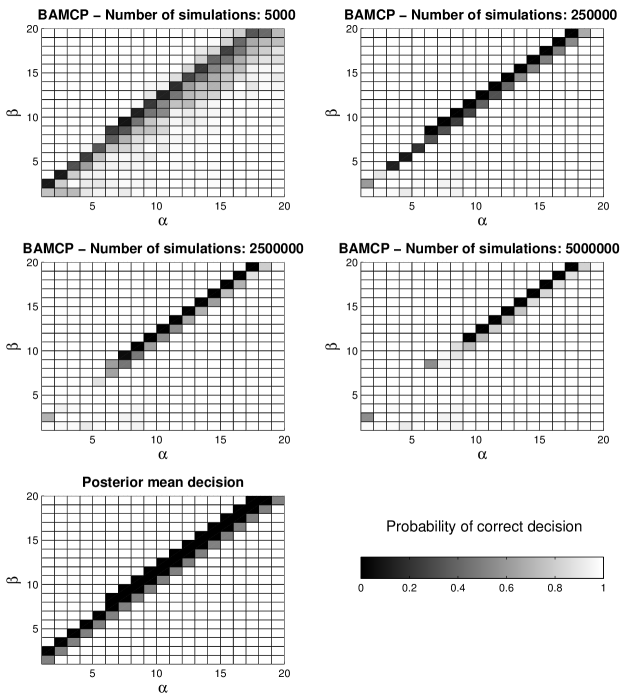
Figure S1: Evaluation of BAMCP against the Bayes-optimal policy, for the case $\gamma=0.95$, when choosing between a deterministic arm with reward $0.5$ and a stochastic arm with reward $1$ with posterior probability $p\sim\text{Beta}(\alpha,\beta)$. The result is tabulated for a range of values of $\alpha,\beta$, each cell value corresponds to the probability of making the correct decision (computed over 50 runs) when compared to the Gittins indices [14] for the corresponding posterior. The first four tables corresponds to different number of simulations for BAMCP and the last table shows the performance when acting according to the posterior mean. In this range of $\alpha,\beta$ values, the Gittins indices for the stochastic arm are larger than $0.5$ (i.e., selecting the stochastic arm is optimal) for $\beta\leq\alpha+1$ but also $\beta=\alpha+2$ for $\alpha\geq 6$. Acting according to the posterior mean is different than the Bayes-optimal decision when $\beta>=\alpha$ and the Gittins index is larger than $0.5$. BAMCP is guaranteed to converges to the Bayes-optimal decision in all cases, but convergence is slow for the edge cases where the Gittins index is close to $0.5$ (e.g., For $\alpha=17,\beta=19$, the Gittins index is $0.5044$ which implies a value of $0.5044/(1-\gamma)=10.088$ for the stochastic arm versus a value of $0.5+\gamma\times 10.088=10.0836$ for the deterministic arm).

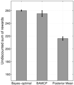
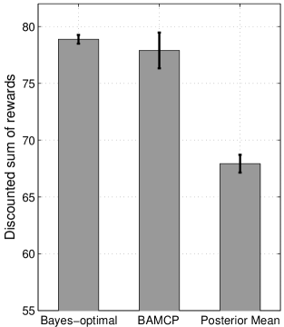
Figure S2: Performance comparison of BAMCP (50000 simulations, 100 runs) against the posterior mean decision on an 8-armed Bernoulli bandit with $\gamma=0.99$ after 300 steps. The arms’ success probability are all $0.6$ except for one arm which has success probability $0.9$. The Bayes-optimal result is obtained from 1000 runs with the Gittins indices [14]. a. Mean sum of rewards after 300 steps. b. Mean sum of discounted rewards after 300 steps.

$\vdots$

$\cdots\begin{array}[]{l}\includegraphics[width=99.37125pt]{infgrid_viz.pdf}\end{array}\cdots$

$\vdots$

Figure S4: A portion of an infinite 2D grid task generated with Beta distribution parameters $\alpha_{1}=1,\beta_{1}=2$ (columns) and $\alpha_{2}=2,\beta_{2}=1$ (rows). Black squares at location (i,j) indicates a reward of 1, the circles represent the corresponding parameters $p_{i}$ (blue) and $q_{j}$ (orange) for each row and column (area of the circle is proportional to the parameter value). One way to interpret these parameters is that following column $i$ implies a collection of $2p_{i}/3$ reward on average ($2/3$ is the mean of a Beta$(2,1)$ distribution) whereas following any row $j$ implies a collection of $q_{j}/3$ reward on average; but high values of parameters $p_{i}$ are less likely than high values parameters $q_{j}$. These parameters are employed for the results presented in Figure 2.

(a)

Inference details for the infinite 2D grid task of Section 5.2

We construct a Markov Chain using the Metropolis-Hastings algorithm to sample from the posterior distribution of row and column parameters given observed transitions, following the notation introduced in Section 5.2. Let $O=\{(i,j)\}$ be the set of observed reward locations, each associated with an observed reward $r_{ij}\in\{0,1\}$. The proposal distribution chooses a row-column pair $(i_{p},j_{p})$ from $O$ uniformly at random, and samples $\operatorname{\tilde{p}}_{i_{p}}\sim\text{Beta}(\alpha_{1}+m_{1},\beta_{1}+n_{1})$ and $\operatorname{\tilde{q}}_{j_{p}}\sim\text{Beta}(\alpha_{2}+m_{2},\beta_{2}+n_{2})$, where $m_{1}=\sum_{(i,j)\in O}\mathbf{1}_{i=i_{p}}r_{ij}$ (i.e., the sum of rewards observed on that column) and $n_{1}=(1-\nicefrac{{\beta_{2}}}{{2(\alpha_{2}+\beta_{2})}})\sum_{(i,j)\in O}\mathbf{1}_{i=i_{p}}(1-r_{ij})$, and similarly for $m_{2},n_{2}$ (mutatis mutandis). The $n_{1}$ term for the proposed column parameter $\operatorname{\tilde{p}}_{i}$ has this rough correction term, based on the prior mean failure of the row parameters, to account for observed $0$ rewards on the column due to potentially low row parameters. Since the proposal is biased with respect to the true conditional distribution (from which we cannot sample), we also prevent the proposal distribution from getting too peaked. Better proposals (e.g., taking into account the sampled row parameters) could be devised, but they would likely introduce additional computational cost and the proposal above generated large enough acceptance probabilities (generally above $0.5$ for our experiments). All other parameters $p_{i},q_{j}$ such that $i$ or $j$ is present in $O$ are kept from the last accepted samples (i.e., $\operatorname{\tilde{p}}_{i}=p_{i}$ and $\operatorname{\tilde{q}}_{j}=p_{j}$ for these $i$s and $j$s), and all parameters $p_{i},q_{j}$ that are not linked to observations are (lazily) resampled from the prior — they do not influence the acceptance probability. We denote by $Q(\operatorname{\mathbf{p}},\operatorname{\mathbf{q}}\rightarrow\operatorname{\mathbf{\tilde{p}}},\operatorname{\mathbf{\tilde{q}}})$ the probability of proposing the set of parameters $\operatorname{\mathbf{\tilde{p}}}$ and $\operatorname{\mathbf{\tilde{q}}}$ from the last accepted sample of column/row parameters $\operatorname{\mathbf{p}}$ and $\operatorname{\mathbf{q}}$. The acceptance probability $A$ can then be computed as $A=\min(1,A^{\prime})$ where:

$$A^{\prime} =\frac{P(\operatorname{\mathbf{\tilde{p}}},\operatorname{\mathbf{\tilde{q}}}|h)Q(\operatorname{\mathbf{\tilde{p}}},\operatorname{\mathbf{\tilde{q}}}\rightarrow\operatorname{\mathbf{p}},\operatorname{\mathbf{q}})}{P(\operatorname{\mathbf{p}},\operatorname{\mathbf{q}}|h)Q(\operatorname{\mathbf{p}},\operatorname{\mathbf{q}}\rightarrow\operatorname{\mathbf{\tilde{p}}},\operatorname{\mathbf{\tilde{q}}})}$$

$$=\frac{P(\operatorname{\mathbf{\tilde{p}}},\operatorname{\mathbf{\tilde{q}}})Q(\operatorname{\mathbf{\tilde{p}}},\operatorname{\mathbf{\tilde{q}}}\rightarrow\operatorname{\mathbf{p}},\operatorname{\mathbf{q}})P(h|\operatorname{\mathbf{\tilde{p}}},\operatorname{\mathbf{\tilde{q}}})}{P(\operatorname{\mathbf{p}},\operatorname{\mathbf{q}})Q(\operatorname{\mathbf{p}},\operatorname{\mathbf{q}}\rightarrow\operatorname{\mathbf{\tilde{p}}},\operatorname{\mathbf{\tilde{q}}})P(h|\operatorname{\mathbf{p}},\operatorname{\mathbf{q}})}$$

$$=\frac{p_{i_{p}}^{m_{1}}(1-p_{i_{p}})^{n_{1}}q_{j_{p}}^{m_{2}}(1-q_{j_{p}})^{n_{2}}\prod_{(i,j)\in O}\mathds{1}[i=i_{p}\text{ or }j=j_{p}](\operatorname{\tilde{p}}_{i}\operatorname{\tilde{q}}_{j})^{r_{ij}}(1-\operatorname{\tilde{p}}_{i}\operatorname{\tilde{q}}_{j})^{1-r_{ij}}}{\operatorname{\tilde{p}}_{i_{p}}^{m_{1}}(1-\operatorname{\tilde{p}}_{i_{p}})^{n_{1}}\operatorname{\tilde{q}}_{j_{p}}^{m_{2}}(1-\operatorname{\tilde{q}}_{j_{p}})^{n_{2}}\prod_{(i,j)\in O}\mathds{1}[i=i_{p}\text{ or }j=j_{p}](p_{i}q_{j})^{r_{ij}}(1-p_{i}q_{j})^{1-r_{ij}}}.$$

The last accepted sampled is employed whenever a sample is rejected. Finally, reward values $R_{ij}$ are resampled lazily based on the last accepted sample of the parameters $p_{i},q_{j}$, when they have not been observed already. We omit the implicit deterministic mapping to obtain the dynamics $\operatorname{\mathcal{P}}$ from these parameters.

References

- [1] J. Asmuth, L. Li, M.L. Littman, A. Nouri, and D. Wingate. A Bayesian sampling approach to exploration in reinforcement learning. In Proceedings of the Twenty-Fifth Conference on Uncertainty in Artificial Intelligence, pages 19–26, 2009.
- [2] J. Asmuth and M. Littman. Approaching Bayes-optimality using Monte-Carlo tree search. In Proceedings of the 27th Conference on Uncertainty in Artificial Intelligence, pages 19–26, 2011.
- [3] R. Bellman and R. Kalaba. On adaptive control processes. Automatic Control, IRE Transactions on, 4(2):1–9, 1959.
- [4] S. Bubeck, R. Munos, and G. Stoltz. Pure exploration in multi-armed bandits problems. In Proceedings of the 20th international conference on Algorithmic learning theory, pages 23–37. Springer-Verlag, 2009.
- [5] P. Castro and D. Precup. Smarter sampling in model-based Bayesian reinforcement learning. In Machine Learning and Knowledge Discovery in Databases, pages 200–214. Springer, 2010.
- [6] P.S. Castro. Bayesian exploration in Markov decision processes. PhD thesis, McGill University, 2007.
- [7] P.A. Coquelin and R. Munos. Bandit algorithms for tree search. In Proceedings of the 23rd Conference on Uncertainty in Artificial Intelligence, pages 67–74, 2007.
- [8] R. Dearden, N. Friedman, and S. Russell. Bayesian Q-learning. In Proceedings of the National Conference on Artificial Intelligence, pages 761–768, 1998.
- [9] M.O.G. Duff. Optimal Learning: Computational Procedures For Bayes-Adaptive Markov Decision Processes. PhD thesis, University of Massachusetts Amherst, 2002.
- [10] AA Feldbaum. Dual control theory. Automation and Remote Control, 21(9):874–1039, 1960.
- [11] N. Friedman and Y. Singer. Efficient Bayesian parameter estimation in large discrete domains. Advances in Neural Information Processing Systems (NIPS), 1(1):417–423, 1 1999.
- [12] S. Gelly, L. Kocsis, M. Schoenauer, M. Sebag, D. Silver, C. Szepesvári, and O. Teytaud. The grand challenge of computer Go: Monte Carlo tree search and extensions. Communications of the ACM, 55(3):106–113, 2012.
- [13] S. Gelly and D. Silver. Combining online and offline knowledge in UCT. In Proceedings of the 24th International Conference on Machine learning, pages 273–280, 2007.
- [14] J.C. Gittins, R. Weber, and K.D. Glazebrook. Multi-armed bandit allocation indices. Wiley Online Library, 1989.
- [15] A. Guez, D. Silver, and P. Dayan. Scalable and efficient Bayes-adaptive reinforcement learning based on Monte-Carlo tree search. Journal of Artificial Intelligence Research, 48:841–883, 2013.
- [16] M. Kearns, Y. Mansour, and A.Y. Ng. A sparse sampling algorithm for near-optimal planning in large Markov decision processes. In Proceedings of the 16th international joint conference on Artificial intelligence-Volume 2, pages 1324–1331, 1999.
- [17] L. Kocsis and C. Szepesvári. Bandit based Monte-Carlo planning. In Machine Learning: ECML, pages 282–293. Springer, 2006.
- [18] J.Z. Kolter and A.Y. Ng. Near-Bayesian exploration in polynomial time. In Proceedings of the 26th Annual International Conference on Machine Learning, pages 513–520, 2009.
- [19] J.J. Martin. Bayesian decision problems and Markov chains. Wiley, 1967.
- [20] N. Meuleau and P. Bourgine. Exploration of multi-state environments: Local measures and back-propagation of uncertainty. Machine Learning, 35(2):117–154, 1999.
- [21] D. Silver and J. Veness. Monte-Carlo planning in large POMDPs. In Advances in Neural Information Processing Systems (NIPS), pages 2164–2172, 2010.
- [22] J. Sorg, S. Singh, and R.L. Lewis. Variance-based rewards for approximate Bayesian reinforcement learning. In Proceedings of the 26th Conference on Uncertainty in Artificial Intelligence, 2010.
- [23] M. Strens. A Bayesian framework for reinforcement learning. In Proceedings of the 17th International Conference on Machine Learning, pages 943–950, 2000.
- [24] C. Szepesvári. Algorithms for reinforcement learning. Synthesis Lectures on Artificial Intelligence and Machine Learning. Morgan & Claypool Publishers, 2010.
- [25] T.J. Walsh, S. Goschin, and M.L. Littman. Integrating sample-based planning and model-based reinforcement learning. In Proceedings of the 24th Conference on Artificial Intelligence (AAAI), 2010.
- [26] T. Wang, D. Lizotte, M. Bowling, and D. Schuurmans. Bayesian sparse sampling for on-line reward optimization. In Proceedings of the 22nd International Conference on Machine learning, pages 956–963, 2005.